Log-periodic behavior in a forest-fire model

SRef-ID: 1607-7946/npg/2005-12-575 European Geosciences Union

© 2005 Author(s). This work is licensed under a Creative Commons License.

Nonlinear Processes

in Geophysics

Log-periodic behavior in a forest-fire model

B. D. Malamud1, G. Morein2, and D. L. Turcotte3

1_{Environmental Monitoring and Modelling Research Group, Department of Geography, King’s College London, Strand,} London, WC2R 2LS, UK

2_{Center for Computational Science and Engineering, University of California, Davis, CA 95616, USA} 3_{Department of Geology, University of California, Davis, CA 95616, USA}

Received: 3 January 2005 – Revised: 29 March 2005 – Accepted: 30 April 2005 – Published: 9 June 2005

Abstract. This paper explores log-periodicity in a forest-fire

cellular-automata model. At each time step of this model a tree is dropped on a randomly chosen site; if the site is unoccupied, the tree is planted. Then, for a given sparking frequency, matches are dropped on a randomly chosen site; if the site is occupied by a tree, the tree ignites and an “in-stantaneous” model fire consumes that tree and all adjacent trees. The resultant frequency-area distribution for the small and medium model fires is a power-law. However, if we con-sider very small sparking frequencies, the large model fires that span the square grid are dominant, and we find that the peaks in the frequency-area distribution of these large fires satisfy log-periodic scaling to a good approximation. This behavior can be examined using a simple mean-field model, where in time, the density of trees on the grid exponentially approaches unity. This exponential behavior coupled with a periodic or near-periodic sparking frequency also generates a sequence of peaks in the frequency-area distribution of large fires that satisfy log-periodic scaling. We conclude that the forest-fire model might provide a relatively simple explana-tion for the log-periodic behavior often seen in nature.

1 Introduction

This paper explores log-periodicity in a forest-fire cellular-automata model. Cellular-cellular-automata (CA) models are lattice-based models which have simple “rules”, but often exhibit complex behavior. At each time step, a series of nearest-neighbour rules of interaction are applied, and individual cells are updated in the next step. A brief history of cellu-lar automata is given by Sarkar (2000). A number of “sim-ple” CA models have been shown to exhibit robust power-law statistics (e.g. for reviews see Turcotte, 1999; Malamud and Turcotte, 2000). Two examples of these include the

sand-Correspondence to: B. D. Malamud

([email protected])

pile model and the forest-fire model, the latter which we will focus on in this paper.

A fractal distribution is a power-law distribution with a real exponent. If the exponent is taken to be a complex num-ber, log-periodic behavior is obtained. In this paper we show that the peaks in the frequency-area distribution of large fires in the forest-fire model can satisfy log-periodic scaling to a good approximation. The possibility of complex scaling ex-ponents and “log periodicity” in critical phenomena has been known for three decades (Nauenberg, 1975) with reviews of log-periodic variabilities given by Sornette (1998, 2002), Jo-hansen and Sornette (2001), and Ide and Sornette (2002). We now briefly review a few specific studies that have proposed spatial and/or temporal log-periodic behavior, including (a) ruptures, (b) seismicity, (c) ground-water, (d) bronchial trees, (e) financial systems, and (f) models:

(a) Ruptures: Anifrani et al. (1995), Johansen and Sornette (2000), and Zhou and Sornette (2002) found that in rup-ture experiments there is a log-periodic relationship be-tween the rate of acoustic emissions as a function of time, prior to the rupture of pressure vessels composed of carbon fibre reinforced resin.

(b) Seismicity: Saleur et al. (1996a) demonstrated a log-periodic increase in the cumulative Benioff strain as a function of time, where the strain is associated with re-gional earthquakes prior to the 17 October 1989 Loma Prieta (California) earthquake (m=7.1). However, this work has been questioned by Huang et al. (2000b) and by Main et al. (2000). In other seismicity studies, Ouil-lon and Sornette (2000) presented data indicating a log-periodic increase in the rate of rockbursts as a function of time, in deep mines in South Africa. Finally, Huang et al. (2000a) argued in favour of log-periodic deviations from Omori’s law in the temporal decay of aftershock activity.

576 B. D. Malamud et al.: Log-periodic behavior in a forest-fire model ground-water chemistry prior to the 1995 Kobe

earth-quake. In other studies, Shibata et al. (2003) found log-periodic variations as a function of time in water levels prior to the 2000 eruption of the Usu Volcano, Japan. (d) Bronchial trees: Schlesinger and West (1991)

demon-strated a log-periodic dependence of mean branch diam-eter as a function of branch orders for bronchial trees. (e) Financial time series: The temporal behavior of

finan-cial time series, including stock indices, exchange rates, and prices, have been argued by a number of authors to exhibit log-periodic fluctuations as a function of time (Feigenbaum and Freund, 1996; Sornette et al., 1996b; Sornette and Johansen, 1997; Johansen and Sornette 1999, 2001; Drozdz et al., 1999, 2003; Zhou and Sor-nette, 2003).

(f) Models: In addition to the “real” world, many theoreti-cal models have also been shown to exhibit log-periodic behavior. For example, Blumenfeld and Ball (1991) modelled a propagating crack and found a spatial log-periodic distribution of corrugations on the crack as a function of the distance from the crack tip. In other rupture studies, Newman et al. (1995) and Sahimi and Arbabi (1996) have shown that models of rupture sim-ulations exhibit log-periodic behaviour. In logistic map studies, Cavalcante et al. (2001) showed that bifurca-tion iterabifurca-tions exhibit log-periodic behavior in the rate of period-doubling on the route to chaos as a func-tion of the value of the control parameter. Similarly, Canessa (2000) found log-periodic variations in a sta-tistical birth-death model. Finally, Saleur et al. (1996b) has related log-periodicity to renormalization group analyses and Sornette et al. (1996a) with the structure of diffusion limited aggregation clusters.

As discussed above, a number of authors have proposed spa-tial and/or temporal log-periodic behavior in engineering ap-plications, natural phenomena, social systems, and models. In this paper, we will examine log-periodic behaviour in the fire model. We first review the sandpile and the forest-fire CA models (Sect. 2), followed by examining the math-ematics of log-periodicity and its application to the forest-fire model (Sect. 3). We then show that the peaks in the frequency-area distribution of large forest-fire model fires satisfy log-periodic behavior (Sect. 4) and finally we advance a mean-field model as a general context within which to un-derstand this log-periodic behavior (Sect. 5). We conclude that the forest-fire model might provide a relatively simple explanation for the log-periodic behavior often seen in na-ture.

2 Two cellular automata models

A classic example of a CA model that exhibits power-law frequency-size statistics of its “output”, is the sandpile model

introduced by Bak et al. (1988). In this model, a square ar-ray of boxes is considered and at each time step a particle is dropped into a randomly selected box. When a box accumu-lates four particles, they are redistributed to the four adjacent boxes, or in the case of edge boxes they are lost from the grid. Because the redistribution involves only the nearest-neighbour boxes, it is a CA model. Redistributions of parti-cles can lead to further instabilities with, at each time step, the possibility of avalanches of particles being lost from the grid. Each of the multiple redistributions during a time step contributes to the size of the model “avalanche”. The size of an avalanche can be associated with the number of parti-cles lost from the grid during the sequence of redistributions or by the number of boxes that participate in the redistribu-tions. Extensive numerical studies of the “sandpile” model were carried out by Kadanoff et al. (1989). They found the noncumulative frequency-size distribution of avalanches to have a power-law distribution with a slope near unity. Bak et al. (1988) used the term “self-organized criticality” (SOC) to classify this type of scaling behavior (see Turcotte 1999 for a review of SOC). Lee and Sornette (2000) used a modi-fied version of the sandpile model and obtained log-periodic scaling of avalanche magnitudes in time.

Another CA model that exhibits this type of scaling behav-ior is the forest-fire model, and is the subject of this paper. The forest-fire model that we use was introduced by Drossel and Schwabl (1992) and has been considered in great detail by Grassberger (2002). This forest-fire model consists of a square grid of sites. At each time step either a model tree or match is dropped on a randomly chosen site. A tree is “planted” only if the site is unoccupied. If a match is dropped on a cell with a tree, the tree ignites and a model fire con-sumes that tree and all adjacent (nondiagonal) trees. For a match dropped on an empty site nothing happens. The spark-ing frequency, f, is the inverse number of attempted tree drops on the square grid before a model match is dropped. If 1/f =100, there have been 99 attempts to plant trees (some successful, some unsuccessful) before a match is dropped at the 100th time step.

On average, the number of trees lost in “fires” is equal to the number of trees planted. However, the number of trees on the grid will fluctuate. The frequency-area distribution of model fires is a statistical measure of the behavior of the sys-tem. The noncumulative frequency-area distribution of small and medium model fires is fractal (power-law) with a slope of about 1.2 (Grassberger, 2002). The forest-fire model is prob-abilistic (stochastic) in that the sites are chosen randomly. It is a cellular-automata model in that only nearest-neighbour trees are ignited by a “burning” tree. In Sect. 4, we will present examples of some model fires and statistical results from our forest-fire model simulations.

-25 -20 -15 -10 -5 0 5 10 15 20 25

0.0 0.1 0.2 0.3 0.4 0.5 0.6 0.7 0.8 0.9 1.0

C= 20,ξ= –2,η= 50

A_A r

A Ar N( )

(b)

-100 -80 -60 -40 -20 0 20 40 60 80 100

0.0 0.1 0.2 0.3 0.4 0.5 0.6 0.7 0.8 0.9 1.0

C= 20,ξ= 0.2,η= 22

A_Ar N( )

A Ar (d) -25

-20 -15 -10 -5 0 5 10 15 20 25

0.0 0.1 0.2 0.3 0.4 0.5 0.6 0.7 0.8 0.9 1.0

C= 20,ξ= 0,η= 22

A_A r

AAr N( )

(c) -25

-20 -15 -10 -5 0 5 10 15 20 25

0.0 0.1 0.2 0.3 0.4 0.5 0.6 0.7 0.8 0.9 1.0

C= 20,ξ= –2,η= 22

A_A r

AAr (a) N( )

Fig. 1. The log-periodic equationN (A/Ar)=C[1−(A/Ar)]−ξcos{−ηln [1−(A/Ar)]}from Eq. (2) is plotted on linear axes,N (A/Ar) as a function ofA/Ar. Shown in each of the four cases are the values chosen for the three constantsC,η, andξ. (i) The effect of changing

η:Candξremain the same, withη =22 in (a),η=50 in (b); the total number of crest-to-crest waves increases with increasingη. (ii) The effect of changingξ:Candηremain the same, withξ = −2 in (a),ξ =0 in (c), andξ =0.2 in (d). Forξ <0 in (a) the waveform amplitudes decrease asA/Ar goes from 0 to 1, compared toξ =0 in (c) where the waveform amplitudes remain the same forA/Ar from 0 to 1, and finallyξ >0 in (d) where the waveform amplitudes increase asA/Ar goes from 0 to 1. For each of the four examples presented in this figure, the sequences of areasA/Ar corresponding to the crests (local maxima, or peaks) of the waveforms are given by Eq. (3).

of time steps in which an attempt is made to plant a tree on an occupied site. However, in general, the frequency-area dis-tributions of all models are similar. This is taken as evidence that the behavior is insensitive to the details of the models; the rules of the cellular-automata models can vary but the re-sults are robust. We will now examine the mathematics of log-periodic scaling in some detail, before returning again to the forest-fire model in Sect. 4.

3 Log-periodic scaling

The concept of fractals was introduced by Mandelbrot (1967) in terms of statistical self-similarity. Given a set of objects or events with different areas, one standard measure (Turcotte, 1997) of fractality is the power-law dependence of number Non areaA,

N (A)∼A−D/2, (1)

whereDis the fractal dimension. Log-periodic scaling fol-lows directly from a complex fractal dimension, D/2 = ξ +iη, with i the square root of minus one, and ξ andη

both real numbers. We again relate the numberNto the area Awith the result (Saleur et al., 1996a)

N (A)=RenCh1− A Ar

i−ξ−iηo

=RenCh1− A Ar

i−ξ

exp−iηlnh1− A Ar

io

=Ch1− A Ar

i−ξ

cos−ηlnh1− A Ar

i

,

(2)

whereRestands for the real part,C ≥ 0 is real and a con-stant, andAr is a reference value ofAwithA < Ar and both

AandAr positive and real.

To aid the reader in visualizing the log-periodic Eq. (2), in Fig. 1 we plot four examples on linear axes forN (A/Ar)

as a function ofA/Ar. We keepC =20 constant in each of

the four examples, and use three different valuesξ = −2.0, 0.0, 0.2 and two valuesη = 22, 50. In each of the four graphs, Eq. (2) results in a quasi-periodic waveform, with the “period” (the horizontal distance between crests of the waveform) decreasing as A/Ar goes from 0 to 1. Figure 1

578 B. D. Malamud et al.: Log-periodic behavior in a forest-fire model

(a)

(b)

(c)

(d)

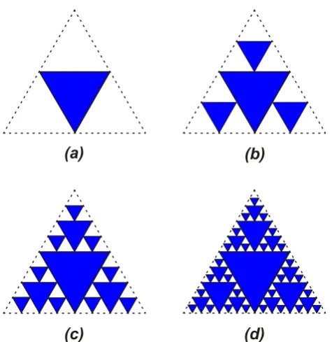
Fig. 2. Four orders of a fractal Sierpinsky gasket. The reference triangle formed by the dashed lines is equilateral and has refer-ence areaAr = 1. (a) At first order this “empty” reference tri-angle is divided into four equal-sized smaller tritri-angles, each with areaA1 = 1/4. The middle triangle is retained (shaded), giving

N1= 1 triangles at order one. This first order acts as a generator

for each successive order, where in each case we go to the remaining “empty” triangles, divide each of them into four equal-sized smaller triangles, and retain (shade) the middle one. In the (b) second or-der we have addedN2 = 3 triangles each with areaA2 = 1/16,

in (c) third orderN3=9 withA3= 1/64, and in (d) fourth order

N4 = 27 withA4 = 1/256. The shaded areas satisfy the

log-periodic sequence given in Eq. (4).

Fig. 1a,η=50 in Fig. 1b, andCandξ remaining the same; we see the total number of crest-to-crest waves increases with increasing η. Figure 1 also demonstrates the effect on the waveform of changing the constantξ in Eq. (2), withξ = −2.0 (Fig. 1a),ξ =0.0 (Fig. 1c),ξ =0.2 (Fig. 1d), andC andηremaining the same. Forξ <0 (Fig. 1a) the waveform amplitudes decrease asA/Ar goes from 0 to 1, compared to

ξ =0 (Fig. 1c) where the waveform amplitudes remain the same forA/Arfrom 0 to 1, and finallyξ >0 (Fig. 1d) where

the waveform amplitudes increase asA/Argoes from 0 to 1.

We note that Eq. (2) gives both positive and negative val-ues ofN (A)as a function ofηandA/Ar. Thus modifications

to this equation must be made where only positive quantities forN (A)are considered. This can be done ifN (A)is a com-bination of the real fractal given in Eq. (1) and the complex fractal given in Eq. (2). However, in the application consid-ered here, we are only interested in the sequence of maxima forN (A)as given by Eq. (2), e.g. the sequence of values of A/Arin Figs. 1a to 1d that correspond to the crests (the local

maxima) for each waveform. We obtain this sequence by let-tingx = [1−(A/Ar)]in Eq. (2) and settingdN (A)/dx=0,

giving (Turcotte, 1997, Eq. 15.42) Ak

Ar

=1−exp

−1

ηtan

−1

_ξ

η

−2kπ

η

,

k=0,1,2,3, ... (3)

withAk the sequence of areasAcorresponding to the

max-ima forN (A). The spacing between successive values ofAk

approaches zero askbecomes large andAk approachesAr.

For the log-periodic behaviour considered in the rest of this paper, we will use Eq. (3).

We next consider a simple geometrical construction that gives the sequence of log-periodic values given by Eq. (3). Consider the fractal Sierpinsky gasket illustrated in Fig. 2. We take the triangular area within the dashed lines to be a reference area withAr =1. The fractal relation (Eq. 1) can

be applied to the number of trianglesNk with areaAk. In

(a) (k =1) we haveN1 = 1,A1 =1/4, in (b) (k =2) we have added N2 = 3, A2 = 1/16, in (c) (k = 3)N3 = 9, A3=1/64, and in (d) (k=4)N4=27,A4=1/256. From Eq. (1) we find that the fractal dimensionD =ln 3/ln 2 ≈

1.585.

We now consider the shaded areas in each of the construc-tions illustrated in Fig. 2. In (a) we have A1/Ar = 1 −

(3/4)=0.250, in (b) we haveA2/Ar =1−(3/4)2≈0.438,

in (c) we haveA3/Ar =1−(3/4)3≈0.578, and in (d) we

haveA4/Ar =1−(3/4)4≈0.684. This result can be

gen-eralized to arbitrary orderkwith the result Ak

Ar =1−

₃

4

k

, k=0,1,2,3, ... (4)

The log-periodic set of areas given in Eq. (3) reduces to the set of areas given in Eq. (4) if we take ξ = 0 and η = 2π/ln(4/3) ≈ 22. This can also be seen in Fig. 1c where Eq. (2) is plotted withξ = 0 andη = 22; the se-quence of values forA/Ar corresponding to local maxima of

N isA/Ar =0, 0.250, 0.438, 0.578, 0.684, 0.763, 0.822, ...,

or in other words the sequence of values given in Eq. (4). Since our original construction is a scale-invariant fractal construction, it is not surprising that the sequence of total areas at each step of the construction obeys a scale-invariant log-periodic law.

The log-periodic sequence of areas corresponding to peaks, as given in Eq. (3), can also be used to predict the reference area and subsequent areas in the sequence. If any three successive values ofAk are observed, i.e.Ai+1,Ai+2, Ai+3,then the reference value,Ar, is given by

Ar =

A2_i+2−Ai+1Ai+3 2Ai+2−Ai+1−Ai+3

. (5)

If we takeAj+1=Ai+1+A0,Aj+2=Ai+2+A0,Aj+3= Ai+3+A0, then Eq. (5) is also satisfied forAj+1,Aj+2and Aj+3. Thus Eq. (5) is independent of origin and can be used for any sequence of threeAk. In addition, the fourth value

in a sequence,Ai+4, is related to the previous three values, Ai+1,Ai+2,Ai+3, by

Ai+4=

A2_i+2+A2_i+3−Ai+1Ai+3−Ai+2Ai+3 Ai+2−Ai+1

We will utilize Eqs. (5) and (6) to show that peaks in the frequency-area distribution of our model fires satisfy log-periodic statistics to a good approximation.

4 Forest-fire model results

The forest-fire model that we consider was described in the introduction. Our forest-fire model is dependent on the size of the square grid, Ng, and the sparking frequency, f. In

our model, fires stop at the edge of the grid and do not wrap around to the other side. A simulation is run forNS time

steps and the number of firesNF with areaAF is determined.

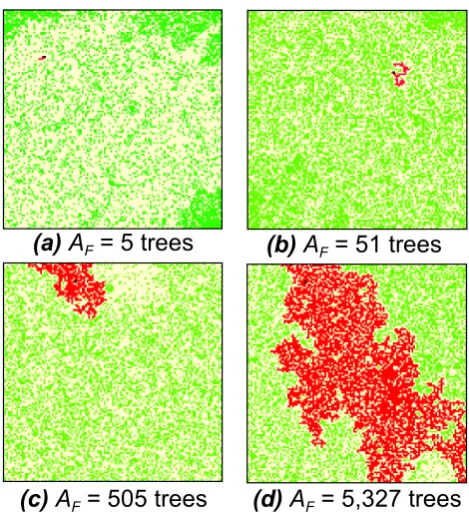
The area is the number of trees that burn in a fire. Examples of four typical fires during a run are given in Fig. 3. In these examples the grid size is 128×128 (Ng =16 384), 1/f =

2000, and fires withAF = 5, 51, 505 and 5327 trees are

illustrated.

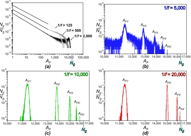
Noncumulative frequency-area statistics for the model fires are given in Fig. 4. The number of fires per time step with areaAF,NF/NS, is given as a function ofAF. In Fig. 4a

results are given for a grid sizeNg =128×128 =16 384

cells and three sparking frequencies, 1/f = 125, 500 and 2000. The small and medium model fires correlate well with the power-law relation

NF

NS

∼A−_Fα (7)

withα=1.0 to 1.2. This is equivalent to the fractal relation (Eq. 1).

For large fires, the frequency-area distribution in Fig. 4 de-viates significantly from a straight-line, such that there is an upper termination to the power-law distribution. In Fig. 4a the deviation is downwards for 1/f = 125 and begins at AF ≈ 800, or 1/20 the size of the grid. At smaller firing

frequencies, the large model fires become more numerous, resulting in an upward deviation from the small fire power-law behavior. For the smallest firing frequency shown in Fig. 4a, 1/f =2000, this deviation begins at approximately AF = 2000, or 1/8 the grid size. When the sparking

fre-quency is very small, large fires become dominant. This can be explained on physical grounds. With a large sparking fre-quency (for example 1/f = 125) trees burn before large clusters can form. If the sparking frequency is very small (for example 1/f =2000) clusters form that span the entire grid before ignition occurs.

An example of a model fire that spans the grid is illus-trated in Fig. 4d (AF =5327). For the simulation with firing

frequency 1/f = 2000 and grid size 128×128, we stud-ied the spanning characteristics of different size model fires and found no fires with sizeAF <2000 span the grid, 50%

of the fires atAF = 3800 span the grid, and all fires with

AF >5300 span the grid. The threshold area at which

clus-ters begin to span a grid will be explored further in Sect. 5, in the context of “percolating” clusters.

In order to examine in more detail the frequency-area dis-tributions of these large clusters we have considered even

(a)

A

= 5 trees

(b)

A

= 51 trees

(c)

A

= 505 trees

(d)

A

= 5,327 trees

Fig. 3. Four examples of typical fires in the forest-fire model are given (figure after Malamud et al., 1998). This run was carried out on a 128×128 grid with 1/f =2000. The red regions are the model fires. The green regions are unburned trees. The white regions are unoccupied grid points. The areasAF of the four model fires are given. The largest model fire is seen to span the entire grid.

smaller firing frequencies. Frequency-area statistics for large fires are given in Figs. 4b to 4d for a 128×128 grid size and sparking frequencies 1/f = 5000, 10 000, and 20 000. It is seen that the model fires cluster at well defined fire areas. For example, for 1/f = 20 000 the clusters peak at AF10 = 11 400, A_F20 = 14 975, A_F30 = 15 970, and

AF40 = 16 260. We use 10, 20, 30, 40 as subscripts for the

successive peaks; these are “any” successive four peaks. The total number of grid sites available isNg =1282=16 384.

The model fires that we observe for the three firing frequen-cies shown in Figs. 4b to 4d are tabulated in Table 1a.

We now utilize Eqs. (5) and (6) derived in the context of log-periodic scaling, in order to see whether the observed forest-fire model peaks satisfy log-periodic behavior. We hy-pothesize that theAr given in Eq. (5) is the total number of

grid sites available,Ar =Ng =16 384. We substitute areas

corresponding to sequences of three observed peaks,AF10,

AF20, A_F30, into Eq. (5) and determineA_r for each of the

observed sequences. For our observed peak sequences we also useAF20,A_F30,A_F40, andA_F30,A_F40,A_F50. The results

calculated forAr are given in Table 1b. It is seen that all

val-ues ofArare close to the hypothesized valueAr=Ng=16 384.

Next, we again use areas corresponding to sequences of three observed peaks, AF10, A_F20, A_F30, andA_F20, A_F30, A_F40,

substitute these two sets of observed values into Eq. (6), and thus derive the next value predicted for each sequence. The predicted values ofAF40 andA_F50 (Table 1c) are in good

580 B. D. Malamud et al.: Log-periodic behavior in a forest-fire model

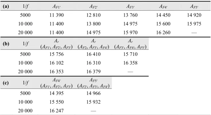
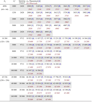
Table 1. (a) Observed peaks in forest-fire model areas∗. (b) Predictions of grid size based on sequences of three observed peaks†. (c) Predictions ofAF40,A_F50 based on sequences of three observed peaks‡.

(a) 1/f AF1′ AF2′ AF3′ AF4′ AF5′

5000 11 390 12 810 13 760 14 450 14 920

10 000 11 400 13 800 14 975 15 600 15 975

20 000 11 400 14 975 15 970 16 260 —

(b) 1/f Ar

(AF1′, AF2′, AF3′)

Ar (AF2, AF3′, AF4′)

Ar (AF3′, AF4′, AF5′)

5000 15 756 16 410 15 710

10 000 16 102 16 310 16 358

20 000 16 353 16 379 —

(c) 1/f AF4′

(AF1′, AF2′, AF3′)

AF5′

(AF2′, AF3′, AF4′)

5000 14 395 14 966

10 000 15 550 15 932

20 000 16 247 —

* _{(a) The peaks in the fire areas A}

F1′, AF2′, AF3′, AF4′, AF5′, illustrated in Figs. 4b to 4d for 1/f = 5000,

10 000, and 20 000 are tabulated. Note that peaks at higher values of AFare present but have not

been tabulated.

† _{(b) The values of A}

r calculated from Eq. (5) are given for sequences of three fire areas from (a) We

associate Ar with the grid area Ng=128 128 16 384× = and find good agreement.

‡ _{(c) The predicted values of A}

F4′ and AF5′ using Eq. (6) are given for observed sequences of three

fire areas from (a). The predicted values are in good agreement with the observed AF4′ and AF5′

given in (a).

5 Mean-field model

In the last section, we showed that for one grid sizeNg =

128×128 and three small firing frequencies, 1/f = 5000, 10 000, 20 000, that the frequency-area distribution of the model fires strongly peak at specific fire areas. These peaks have been illustrated in Figs. 4b to 4d, and tabulated in Ta-ble 1a. We now extend our studies to smaller and larger grid sizes,Ng=64×64 andNg=256×256, and firing

frequen-cies from 1/f =1000 to 160 000. The values of the observed peaks for these studies are tabulated in Table 2. Our objective is to provide a model to explain the distribution of peaks.

The peaks we wish to study occur only at very small values of the firing frequency. For small firing frequencies the loss of trees occurs primarily in large grid-spanning fires. After a very large fire we assume it is a good approximation to set the number of trees on the grid,At, to be zero and take this

to be the time origin, thusAt =0 att =0. In this limit the

behavior of the forest-fire model is identical to the behavior of the site-percolation model (Stauffer and Aharony, 1992). In this case it is appropriate to make a mean-field approxi-mation for the increase in the number (total area)At of trees

on the grid with time. Althought increases in discrete time steps of1t = 1, we can approximate this increase by the continuum relation

dAt

dt =1− At

Ng

. (8)

Initially At, the number of trees on the grid, is small and

dAt/dt ≈ 1; therefore, a tree is planted at every time step.

Subsequently the probability that a tree is planted at a time step is[1−(At/Ng)]. Solving Eq. (8) withAt =0 andt =0

we obtain At

Ng

=1−exp

− t

Ng

. (9)

In other words, without fires the density of trees on the grid At/Nginitially increases rapidly with timet, with the rate of

increase decreasing exponentially and an asymptotic limit of 1 tree per cell (a fully occupied grid).

Matches are dropped at timest =k/f,k=1, 2, 3, 4, . . . . Using this expression andAF k =At in Eq. (9), then the set

of fire sizes corresponding to these match drops is AF k

Ng

=1−exp

− k

f Ng

, k=1,2,3,4, ... (10) Note that the succession of theoretical peaksAF k = AF1, AF2,AF3,AF4, . . . are not necessarily the same set of suc-cessive observed peaks as discussed in the last sectionAF10,

AF20,A_F30,A_F40, . . . ; this is discussed further below. The

fire areasAF kapproach the grid sizeNgaskbecomes large.

Associating the grid sizeNg in Eq. (10) with the reference

areaAr in Eq. (3) and takingξ = 0 andη = 2πf Ng, the

1 10 100 1,000 100,000

10,000 11,000 12,000 13,000 14,000 15,000

1/f= 125 1/f= 500 10-3

10-4

10-5 10-6

10-7 10-8

10-9 10-10

AF

1/f= 2,000

(a)

10,000 11,000 12,000 13,000 14,000 15,000

11//ff== 1100,,000000

AF1′ _A

F2′

A_F3′

AF4′

A_F5′

AF (c)

10,000 11,000 12,000 13,000 14,000 15,000

11//ff== 55,,000000

A_F1′

A_F3′ AF4′

A_F5′

AF A_F2′

(b)

11//ff== 2200,,000000

A_{F1′ A}

F2′

A_F3′

AF4′

AF (d) 10-6

10-7

10-8

10-9

NF

N_S

10-6

10-7

10-8

10-9

10-6

10-7

10-8

10-9 N_F N_S

N_F N_S NF

N_S

N Ngg

10,000 17,000

N Ngg

16,000

17,000

16,000 16,00017,000

Fig. 4. Frequency-area statistics of the forest-fire model. (a) The number of fires per time stepNF/NSwith areaAF (number of lattice cells in the “fire”), is given as a function ofAF (Fig. 4a after Malamud et al., 1998). Results are given for a grid withNg=128×128, and firing frequencies 1/f =125, 500, and 2000. To further investigate the behavior of the distribution for the very large fires, we again use grid size

Ng = 128×128 and focus in on the area fromAF = 10 000 toAF =17 000 for three different firing frequencies (b) 1/f = 5000, (c) 1/f =10 000, and (d) 1/f =20 000. Marked in each figure are the observed peaks that occur,AF10,A_F20,A_F30, ..., and the location on the horizontal axis forAF =Ng.

the areasAk given in Eq. (3). This simple model predicts a

log-periodic distribution of fire peaks.

In Table 2 we give a wide range of observed peaks (AF

observed) obtained from forest-fire model simulations. Grid sizes 64×64 (Ng =4096), 128×128 (Ng =16 384), and

256×256 (Ng =65 536) have been considered. Firing

fre-quencies range from 1/f = 1000 to 160 000. Numbers of observed peaks range from two to seven. The observed val-ues previously given in Table 1a for 1/f =5000 and 20 000 are also included. Using the values of Ng and f used in

each simulation, theoretical predicted values of peak areas AF k are obtained from the log-periodic mean-field relation

(Eq. 10) for various values ofk. These are given in Table 2 asAF k theoretical, withk given in brackets. It is seen that

there is excellent agreement between the mean field predic-tions and the values observed in the forest-fire model simu-lations.

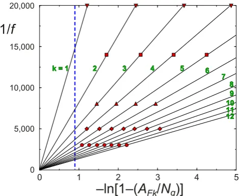
The results given in Table 2 are also illustrated in Fig. 5. The mean-field results given in Eq. (10) can be rewritten as

−ln

1−AF k Ng

= k

f Ng

, k=1,2,3,4, ... (11) In Fig. 5, the dependence of 1/f on−ln

1− AF k/Ngis

shown forNg = 128×128 and k = 1 to 12 using solid

straight lines. Also included in Fig. 5 as data points are the observed peaks from our forest-fire model simulations as given in Table 2 forNg=128×128 and five values of 1/f.

It is seen that the sequence of areas corresponding to peaks

in the simulations closely agree with the sequence of areas given by increasing integer values ofkin our mean-field pre-diction from Eq. (11).

We now address 10, 20, 30, ... in sequences of observed areasAF10,A_F20,A_F30, ..., not necessarily corresponding to

k=1, 2, 3, ... in theoretical areasAF k. Specifically, consider

Ng =128×128=16 384 cells, and 1/f =5000, as given

in Table 1a. Comparing with Table 2, we findAF10 (i.e. the

first observable peak area) corresponds toAF4(i.e. the fourth theoretical peak area), AF20 corresponds to A_F5, etc. The

peaks associated withk =1, 2, 3 are “missing”. To explain this we introduce the concept of percolating clusters.

A percolating cluster corresponds to a cluster of trees that span the grid. At any given time, more than one span-ning cluster on the grid can only occur on very rare oc-casions. From studies of site percolation we can conclude that the “threshold” for a spanning cluster occurring ispc =

At c/Ng =0.59275 (Stauffer and Aharony, 1992) whereAt c

is the number of trees in the spanning clusters. Substituting At cforAF kin Eq. (11), andAt c/Ng=0.59275, we find that

at the percolation threshold,−ln[1−(At c/Ng)] =0.8983.

582 B. D. Malamud et al.: Log-periodic behavior in a forest-fire model

Table 2. Theoretical peaks forAF kcompared to observed peaks∗.

Ng 1/f Spanning

Cluster† A_(AFk_F Theoretical [ _Observed) k]

4096 1000 2428 2888 [5] 3149 [6] 3354 [7] 3515 [8] 3641 [9] 3739 [10] 3817 [11] (64 × 64) 2845 3146 3350 3513 3660 3744 3835

1250 2428 2888 [4] 3205 [5] 3440 [6] 3612 [7] 3739 [8] 3833 [9] 3902 [10] 2840 3200 3440 3615 3743 3816 3890 2000 2428 3149 [3] 3515 [4] 3739 [5] 3877 [6] 3962 [7]

3140 3521 3743 3883 3965

5000 2428 2888 [1] 3739 [2] 3991 [3] 4065 [4] 4087 [5] 2850 3747 3993 4065 4088

10 000 2428 3739 [1] 4065 [2] 4093 [3] 3742 4066 4093

16 384 3000 9712 10 923 [6] 11 837 [7] 12 597 [8] 13 231 [9] 13 759 [10] 14 198 [11] 14 564 [12] (128 × 128) 10 600 11 750 12 597 13 227 13 745 14 218 14 588

5000 9712 11 550 [4] 12 822 [5] 13 759 [6] 14 449 [7] 14 958 [8] 15 333 [9] 15 609 [10] 11 390 12 810 13 760 14 450 14 920 15 317 15 628 8000 9712 12 597 [3] 14 060 [4] 14 958 [5] 15 509 [6]

12 560 14 080 14 960 15 530 14 000 9712 13 418 [2] 15 122 [3] 15 847 [4] 16 155 [5]

13 400 15 130 15 860 16 150 20 000 9712 11 550 [1] 14 958 [2] 15 963 [3] 16 260 [4]

11 400 14 975 15 970 16 260 100 000 9712 16 347 [1] 16 384 [2]

16 348 16 384

65 536 20 000 38 846 46 201 [4] 51 287 [5] 55 034 [6] 57 796 [7] 59 832 [8] (256 × 256) 45 560 51 250 55 100 57 770 59 900

40 000 38 846 46 201 [2] 55 034 [3] 59 832 [4] 62 438 [5] 63 853 [6] 45 630 55 100 59 880 62 430 63 850

80 000 38 846 46 201 [1] 59 832 [2] 63 853 [3] 65 040 [4] 65 390 [5] 45 630 59 875 63 855 65 065 65 400

160 000 38 846 59 832 [1] 65 040 [2] 65 493 [3] 59 800 65 040 65 494

* Included in this table are the values predicted (AFk theoretical) using the mean-field results given

in Eq. (10) with the value of k used given in square brackets. Also included are the observed peaks

(AF observed) obtained from forest-fire simulations for three grid sizes, 64 64× (Ng=4096)

128 128× (Ng=16 384) and 256 256× (Ng=65 536), and a variety of firing frequencies

1/f = 1000 to 160 000.

† The spanning cluster is equal to 0.59275 Ng and is the critical value below (or nearby) which peaks

in AF are not observed.

actuality, theoretical peaks slightly greater than this percolat-ing threshold cluster, although they occur, can be difficult to observe.

As an example, we take the case discussed previously (Ng =128×128 and 1/f =5000). In Fig. 5, we see from

the row of diamonds, that the peaks corresponding tok=1, 2, 3 are “missing”. As another example, consider the data for 1/f =3000 andNg =128×128 in Table 2. The smallest

observed peak for fire areas is atAF10 =10 600. This

cor-responds to−ln[1−(AF/Ng)] =1.041 which is above the

percolation threshold of 0.8983, and agrees with the theoreti-cal predicted peakAF6=10 923 from Eq. (11) usingk=6,

1/f =3000 andNg =128×128. The predicted peaks for

k =1, ..., 5 do not occur, as the location of these peaks are less than the spanning clusters, so they do not show up as peaks. Peaks in the distribution of fires occur only when the density of trees on the grid is greater than the critical density for grid spanning clusters.

behav-ior. The large model fires peak only when the density of trees on the grid exceeds the percolation threshold for tree clusters that span the grid. These spanning clusters are responsible for the peaks that we see in our distribution of fire areas, with at any given time only one spanning cluster on the grid. If the first match dropped after the percolation threshold is reached hits a tree, a fire corresponding to the peak with the small-est area is observed. If the first match misses a tree then the spanning cluster grows exponentially as shown in Eq. (9). If the second match hits a tree, a fire in the peak with the next largest peak area is observed, and so forth. The exponen-tial growth of cluster areas asymptotically approaching the size of the grid, combined with a periodic (or near periodic) sparking frequency, are necessary conditions for robust log-periodic behavior.

6 Conclusions

Many natural phenomena are associated with “avalanches” that satisfy power-law (fractal) frequency-magnitude distri-butions to a good approximation. Examples include land-slides (Guzzetti et al., 2002; Malamud et al., 2004), earth-quakes (Aki, 1981; Turcotte and Malamud, 2002), and wild-fires (Malamud et al., 1998, 2005; Ricotta et al., 1999). These examples are also closely associated with simple cel-lular automata that are said to exhibit self-organized critical-ity (Bak et al., 1988). Landslides with the sandpile model, earthquakes with the slider-block mode, and wildfires with the forest-fire model.

In this paper we have studied the behavior of the forest-fire model when the firing frequency is very small. Trees are planted until they form a large cluster that spans the square grid of planting sites. These large clusters are “burned” when matches are dropped at large prescribed intervals. We have focused our attention on the frequency-area distribution of these very large fires. This distribution is characterized by a series of very well defined peaks which become more closely spaced with increasing fire size. We have shown that these peaks satisfy log-periodic scaling to a very good approxima-tion. A log-periodic distribution can be obtained by taking a power-law (fractal) distribution and making the power-law exponent (the fractal dimension) a complex number.

We have also shown that a very simple mean-field model produces the log-periodic peaks seen in our forest-fire simu-lations. Without any fires the forest-fire model is identical to the site percolation model, where the number of trees (area) on the grid initially increases rapidly with time (1 tree per time step), with the rate of increase decreasing exponentially as the grid fills up. If trees are then destroyed (burned) at equally spaced time intervals, the areas have a log-periodic distribution of fire sizes.

As discussed in the introduction, log-periodic distributions are often seen in nature and in numerical simulations. The studies presented here illustrate circumstances in which log-periodicity can be expected. First a characteristic size is re-quired. For the forest-fire model, this is the area of the grid.

0 5,000 10,000 15,000 20,000

0 1 2 3 4 5

1/

f

77 88 99 1100 1111 1122

kk == 11 22 33 44 55 ₆₆

–ln[1–(

A

/

N

)]

Fig. 5. The predicted mean-field dependence of the firing frequency 1/f is given as a function of−ln[1−(AF k/Ng)]. Solid straight lines are from −ln[1−(AF k/Ng)] = (k/f Ng) (Eq. 11) for twelve different values ofkandNg =128×128. The data points (triangles, squares, diamonds and circles) are the observed peaks (AF observed, in Table 2) for 1/f = 3000, 5000, 8000, 14 000, 20 000 andNg =128×128. The agreement between “observed” and “predicted” values, also seen in Table 2, is clearly illustrated in this figure. The vertical dashed line at−ln[1−(A_{F k}/Ng)] = 0.89833 represents the percolation model threshold at which the spanning cluster area isAt c = 0.59275×Ng = AF k. To the left of this vertical line, peaks in the frequency-area distribution are not observed for the forest-fire model.

Second, the trigger for the “avalanches” must be periodic or near periodic. In the forest-fire model, the periodic triggers are the regular spaced match drops. We conclude that the forest-fire model might provide a relatively simple explana-tion for the log-periodic behavior often seen in nature. Acknowledgements. The contributions of author DLT were partially supported by NSF Grant NO ATM 0327558 and the contributions of author BDM were partially supported by the UK NERC/EPSRC Grant NER/T/S/2003/00128. We also thank the two referees, S. Hergarten and one person who remained anonymous, for their very helpful comments.

Edited by: G. Z¨oller

Reviewed by: S. Hergarten and another referee

References

Aki, K.: A probabilistic synthesis of precursory phenomena, in: Earthquake Prediction, edited by: Simpson, D. W. and Richards, P. G., Maurice Ewing Series 4, American Geophysical Union: Washington, D. C., 566–574, 1981.

584 B. D. Malamud et al.: Log-periodic behavior in a forest-fire model

Bak, P., Tang, C., and Wiesenfeld, K.: Self-organized criticality, Phys. Rev. A, 38, 364–374, 1988.

Bak, P., Chen, K., and Tang, C.: A forest-fire model and some thoughts on turbulence, Phys. Let. A, 147, 297–300, 1992. Blumenfeld, R. and Ball, R. C.: Onset of scale-invariant pattern in

growth processes: the cracking problem, Physica A, 177, 407– 415, 1991.

Canessa, E.: Stochastic theory of log-periodic patterns, J. Phys. A, 33, 9131–9140, 2000.

Cavalcante, H. L. D. D., Vasconcelos, G. L., and Leite, J. R. R.: Power law periodicity in the tangent bifurcations of the logistic map, Physica A, 295, 291–296, 2001.

Christensen, K., Flyvbjerb, H., and Olami Z.: Self-organized criti-cal forest-fire model: Mean-field theory and simulation results in 1 to 6 dimensions, Phys. Rev. Let., 71, 2737–2740, 1993. Clar, S., Drossel, B., and Schwabl, F.: Forest fires and other

exam-ples of self-organized criticality, J. Phys. Condensed Matter, 8, 6803–6824, 1996.

Drossel, B. and Schwabl, F.: Self-organized critical forest-fire model, Phys. Rev. Let., 69, 1629–1632, 1992.

Drossel, B. and Schwabl, F.: Formation of space-time structure in a forest-fire model, Physica A, 204, 212–229, 1994.

Drozdz, S., Ruf, F., Speth, J., and Wojcik, W.: Imprints of log-periodic self-similarity in the stock market, Eur. Phys. J. B, 10, 589–593, 1999.

Drozdz, S., Grummer, F., Ruf, F., and Speth, J.: Log-periodic self-similarity: an emerging financial law?, Physica A, 324, 174–182, 2003.

Feigenbaum, J. A. and Freund, P. G. O.: Discrete scale invariance in stock markets before crashes, Int. J. Mod. Phys. B, 10, 3737– 3745, 1996.

Grassberger, P.: Critical Behavior of the Drossel-Schwabl Forest Fire Model, New J. Phys., 4, 17.1–17.15, 2002.

Guzzetti, F., Malamud, B. D., Turcotte, D. L., and Reichenbach, P.: Power-law correlations of landslide areas in central Italy, Earth Plan. Sci. Lett., 195, 169–183, 2002.

Henley, C. L.: Statics of a “self-organized” percolation model, Phys. Rev. Let., 71, 2741–2744, 1993.

Huang, Y., Johansen, A., Lee, M. W., Saleur, H., and Sornette, D.: Artifactual log-periodicity in finite size data: relevance for earth-quake aftershocks, J. Geophys. Res., 105, 25 451–25 471, 2000a. Huang, Y., Saleur, H., and Sornette, D.: Reexamination of log pe-riodicity observed in the seismic precursors of the 1989 Loma Prieta earthquake, J. Geophys. Res., 105, 28 111–28 123, 2000b. Ide, K. and Sornette, D.: Oscillatory finite-time singularities in

fi-nance, population and rupture, Physica A, 307, 63–106, 2002. Johansen, A.: Spatio-temporal self-organization in a model of

dis-ease spreading, Physica D, 78, 186–193, 1994.

Johansen, A. and Sornette, D., Modeling the stock market prior to large crashes, Eur. Phys. J. B, 9, 167–174, 1999.

Johansen, A. and Sornette, D.: Critical ruptures, Eur. Phys. J. B, 18, 163–181, 2000.

Johansen, A. and Sornette, D.: Finite-time singularity in the dy-namics of the world population, economic and financial indices, Physica A, 294, 465–502, 2001.

Johansen, A., Saleur, H., and Sornette, D.: New evidence of quake precursory phenomena in the 17 January 1995 Kobe earth-quake, Japan, Eur. Phys. J. B, 15, 551–555, 2000.

Kadanoff, L. P., Nagel, S. R., Wu, L., and Zhou, S. M.: Scaling and universality in avalanches, Phys. Rev. A, 39, 6524–6533, 1989. Lee, M. W. and Sornette, D.: Novel mechanism for discrete scale

in-variance in sandpile models, Eur. Phys. J. B, 15, 193–197, 2000.

Malamud, B. D., and Turcotte D. L.: Cellular-automata models ap-plied to natural hazards, IEEE Comp. Sci. Eng., 2, 42–51, 2000. Malamud, B. D., Morein, G., and Turcotte, D. L.: Forest fires: an example of self-organized critical behavior, Science, 281, 1840– 1842, 1998.

Malamud, B. D., Turcotte, D. L., Guzzetti, F., and Reichenbach, P.: Landslide inventories and their statistical properties, Earth Surf. Proc. Landforms, 29, doi:10.1002/esp.1064, 687–711, 2004. Malamud, B. D., Millington, J. D. A., and Perry G. L. W.:

Charac-terizing wildfire regimes in the USA, Proc. Nat. Acad. Sci., 102, 4694–4699, 2005.

Main, I. G., O’Brien, G., and Henderson, J. R.: Statistical physics of earthquakes: comparison of distribution exponents for source area and potential energy and the dynamic emergence of log-periodic energy quanta, J. Geophys. Res., 105, 6105–6126, 2000. Mandelbrot, B.: How long is the coast of Britain? Statistical self-similarity and fractional dimension, Science, 156, 636–638, 1967.

Mossner, W. K., Drossel, B., and Schwabl, F.: Computer simula-tions of the forest-fire model, Physica A, 190, 205–217, 1992. Nauenberg, M.: Scaling representation for critical phenomena, J.

Phys. A, 8, 925–928, 1975.

Newman, W. I., Turcotte, D. L., and Gabrielov, A. M.: Log-periodic behavior of a hierarchical failure model with applications to pre-cursory seismic activation, Phys. Rev. E., 52, 4827–4835, 1995. Ouillon, G. and Sornette, D.: The concept of “critical earthquakes”

applied mine rockbursts with time-to-failure analysis, Geophys. J. Int., 143, 454–488, 2000.

Ricotta, C., Avena, G., and Marchetti M.: The flaming sandpile: self-organized criticality and wildfires, Ecol. Model., 119, 73– 77, 1999.

Sahimi, M. and Arbabi, S.: Scaling laws for fracture of heteroge-neous materials and rock, Phys. Rev. Let., 77, 3689–3692, 1996. Saleur, H., Sammis, C. G., and Sornette, D.: Discrete scale invari-ance, complex fractal dimensions, and log-periodic fluctuations in seismicity, J. Geophys. Res., 101, 17 661–17 677, 1996a. Saleur, H., Sammis, C. G., and Sornette, D.: Renormalization

group theory of earthquakes, Nonlin. Proc. Geophys., 3, 102– 109, 1996b, SRef-ID: 1607-7946/npg/1996-3-102.

Sarkar, P.: A brief history of cellular automata, ACM Computing Surveys, 32, 80–107, 2000.

Schlesinger, M. F. and West, B. J.: Complex fractal dimension of the bronchial tree, Phys. Rev. Let., 67, 2106–2108, 1991. Shibata, T., Matsumoto, N., and Akita, F.: Fluctuation in

groundwater level prior to the critical failure point of the crustal rocks, Geophys. Res. Let., 30, 1, art. no. 1024, doi:10.1029/2002GL016050, 2003.

Sornette, D.: Discrete-scale invariance and complex dimension, Phys. Reports, 297, 239–270, 1998.

Sornette, D.: Predictability of catastrophic events: material rup-ture, earthquakes, turbulence, financial crashes, and human birth, Proc. Nat. Acad. Sci., 99, 2522–2529, 2002.

Sornette, D. and Johansen, A.: Large financial crashes, Physica A, 245, 411–422, 1997.

Sornette, D., Johansen, A., Arneodo, A., Muzy, J. F., and Saleur, H.: Complex fractal dimensions describe the hierarchical structure of diffusion-limited-aggregate clusters, Phys. Rev. Let., 76, 251– 254, 1996a.

Sornette, D., Johansen, A., and Bouchaud, J. P.: Stock market crashes, precursors and replicas, J. Phys. I France, 6, 167–175, 1996b.

2nd ed., Taylor and Francis, London, 1992.

Turcotte, D. L. Fractals and Chaos in Geology and Geophysics, 2nd ed., Cambridge University Press, Cambridge, 1997.

Turcotte, D. L.: Self-organized criticality, Reports on Progress in Physics, 62, 1377–1429, 1999.

Turcotte, D. L. and Malamud, B. D.: Earthquakes as a complex sys-tem, in: International Handbook of Earthquake and Engineering Seismology, edited by: Lee, W. H. K, Kanamori, H., Jennings, P. C., and Kisslinger, C., Academic Press: London, 209–227, 2002.

Zhou, W. X. and Sornette, D.: Generalized q analysis of log-periodicity: applications to critical ruptures, Phys. Rev. E, 66, art. no. 046111, 8 p., 2002.