Conditional Inference for the Weibull Extension Model Based on the Generalized Order Statistics

(1)

on the Generalized Order Statistics

M. Maswadah

Department of Mathematics, Faculty of Science, Aswan University, Egypt [email protected]

A. A. EL-Faheem

Department of Mathematics, Faculty of Science, Aswan University, Egypt [email protected]

Abstract

In recent years, a new class of models has been proposed to exhibit the bathtub-shaped failure rate functions. The Weibull extension model is one of these models, which is asymptotically related to the ordinary Weibull model and is capable of modeling the bathtub-shaped and increasing failure rate lifetime data. This paper presents the conditional inference for constructing the confidence intervals for the Weibull extension parameters based on the generalized order statistics. For measuring the performances of this approach comparing to the Asymptotic maximum likelihood estimates, Simulation studies have been carried out, that indicated the conditional intervals possess a good statistical properties and they can perform quite well even when the sample size is extremly small. An illustrative examples based on real data are given to illustrate the confidence intervals developed in this paper.

Keywords: Weibull extension model; Modified Weibull model; Weibull distribution; Burr-type XII distribution; Lamox distribution; Generalized Pareto model; Progressive type-II censored samples with binomial random removals; Asymptotic maximum likelihood estimates.

1. Introduction

In the last decade, a new class of distributions has been proposed based on extended forms of the Weibull distribution to provide a better fitting than the Weibull distribution. This class has been studied extensively in the literature for its various applications in reliabiliy and life-data statistics and modeling the lifetimes of electro-mechnical, electronic and mechanical products. Aarset (1987) discussed the identification of the bathtub-hazrd rate function. Xie and Lai (1996) studied the reliability analysis for the bathtub-shaped failure rate function. Wang et al. (2002) presented a general form for the bathtub shaped hazard function in terms of reliability. Lai et al. (2003) discussed in details the bathtub-shaped failure rate life distributions.

Chen (2000) introduced the Weibull extension model as a new lifetime distribution that has bathtub-shaped hazard rate function and discussed some characteristics of this model and explained its cabiblity for describing the life time variables of bathtub-shaped hazard rate function. The cumulative distribution function of the Weibull extension model (WEM ) is given by

))

1

)

(exp(

exp(

1

)

(

x

=

−



x



−

F

_,



,



,

x



0

,

(1.1)

(2)

Xie et al. (2002) presented the WEM as a distribution with the property of bathtub-shaped failure rate function. Tang et al. (2003) carried out in details the statistical analysis of this distribution and they derived the confidence intervals based on the asymptotic maximum likelihood estimates (AMLEs). Wu et al. (2004) derived the exact confidence interval for shape parameter. Pham and Lai (2007) discussed most of the modifications for the Weibull distribution, and Silva et al. (2009) derived the maximum likelihood estimates (MLEs) for the parameters of this model and presented some inferential procedures. This paper extends the analysis on the Weibull extension model by introducing the conditional inference procedures as a tool for constructing the confidence intervals for the parameters based on the generalized order statistics. However, the conditional approach as proposed by Sir Fisher (1934) has been applied for many lifetime distributions belonging to the location-scale family, see Lawless (1973, 1974, 1975, 1978, 1980, 1982) or those can be transformed to this family, see Maswadah (2003, 2005). Thus as a new application for the conditional approach, the conditional confidence intervals for the shape-scale family parameters have been constructed based on the generalized order statistics. The cumulative distribution function (cdf) and probability density function (pdf) for the shape-scale family are given, respectively, by:

))

(

exp(

1

)

(

x

g

x

F

=

−



 ,



,



,

x



0

, (1.2)

))

(

exp(

)

(

)

(

)

(

x

g

1

x

g

x

g

x

f

=



−



−



 ,



,



,

x



0

(1.3)

For convenience we assume

g

(

x

)

to be differentiable as well as strictly increasing

function of

x

,

g

(

0

+

)

=

0

and

g

(

x

)

→



as

x

→



.

The parameters  and  are shape and scale respectively.

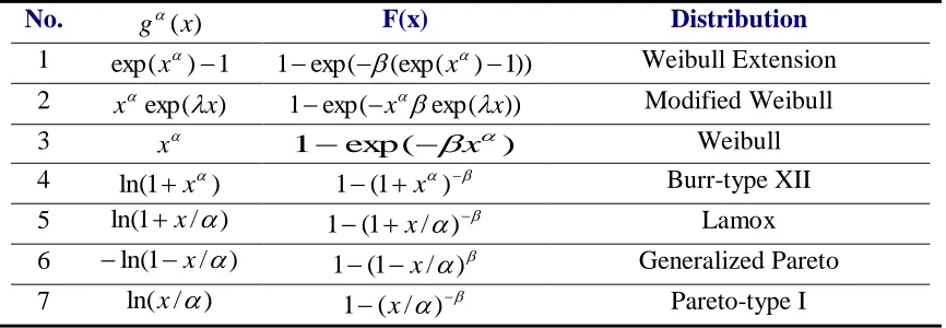
This family includes among others the most popular parameteric models in lifetime distributions such as the Weibull extension model, modified Weibull model, Weibull distribution, Pareto distribution, Burr-type-XII distribution, Lamox distribution and the

Generalized Pareto distribution according to the values of

g



(

x

)

. Some important members of this family are shown in Table 1.

Table 1:

No. _g₍_x₎ F(x) Distribution

1 exp(x)−1 1−exp(−(exp(x)−1)) Weibull Extension

2 _x _exp(_x₎ ₁−_exp(−_x_exp(_x₎₎ Modified Weibull

3 _x ₁−_{exp (}−_x₎ Weibull

4 _ln(₁+_x₎ ₁−₍₁+_x₎− Burr-type XII

5 ln(1+x/) ₁₋₍₁₊_x_/₎− Lamox

(3)

For the importance of this family, the conditional inference has been proposed for constructing the confidence intervals for its parameters based on the generalized order statistics (GOS), that introduced by Kamps (1995) as a unified approach to ordinary OS, progressive type-II OS, record values and k-th record values, which can be outlined as:

Let

F

(

x

)

be an absolutely continuous function with pdf

f

(

x

)

. The random variables

)

,

~

,

(

),....,

,

~

,

1

(

n

m

k

X

n

m

k

X

are called GOS, with noting thatX(0,n,m~,k)=0,

1



k , if their joint pdf can be written in the form:



 





− = −

−

=

1 1 2

1

,

,...,

)

(

)

1

(

)

1

(

)

(

)

(

1 n i n n i i

n

C

f

x

F

x

F

x

f

x

f

i k

m

,

(1.4)

on the cone

F

−

1

(

0

)



x

1



....



x

n



F

−

1

(

1

)

of Rn, where

1 n i i C  = =



, i i =k+n−i+M



,



−

=

= n 1

i j

j

i m

M _, n =k 0, and 1

1 2

1, ,..., )

( ~ − −  = n n R m m m m

represents the number of units withdrawn at the corresponding failure times.

• If

m

~

=

0

and

k

=

1

then (1.4) is the joint pdf of the ordinary order statistics.

• If

m

~

=

0

and

m

n

=

k

−

1

and



=

+

=

n i i

m

n

N

1

then (1.4) is the

joint pdf of the type-II censored order statistics.

• If

m

~



0

,

m

n

=

k

−

1

and



=

+

=

n i i

m

n

N

1

then (1.4) is the joint

pdf of the type-II progressively censored order statistics.

2. Conditional inference methodology

For the first time, we will give outline for the conditional approach to inference on the shape-scale family (1.2).

Given a set of

n

GOS

X

(

1

,

n

,

m

~

,

k

),....,

X

(

n

,

n

,

m

~

,

k

)

with sampling density function belonging to (1.2), thus by substituting (1.2 ) and (1.3) in (1.4) we can derive the joint pdf as













−

+

−



=





₌ = −

))]

(

)

1

(

)

(

)

1

(

exp[

)

(

)

(

)

,...,

(

₁ 1 1 1 n n n i i i n i i i n n n

x

g

m

k

x

g

m

x

g

x

g

C

x

f

  





_. (2.1)

For the shape-scale family (1.2), if ˆ and ˆ_{be any equivariant estimators such as the} MLEs of  and  , then

Z

₁

=



/



ˆ

and



1/ 1

/



ˆ

2

z

(4)

)

(

ˆ

i

g

x

a

=





,

i

=

1

,

2

,...,

n

form a set of ancillary statistics. Thus based on the following theorem, we can derive the conditional densities for the pivotal quantities conditional on the ancillary statistics and the confidence intervals can be constructed and converting them for  and  fiducially.

Theorem:

Let ˆ and ˆ be any equivariant estimators of  and  for the shape-scale family (1.2), based on the generalized order statistics

X

(

1

,

n

,

m

~

,

k

),....,

X

(

n

,

n

,

m

~

,

k

)

. Then

the conditional pdf of Z₁ and Z₂ given

(

,

,...,

)

2 2

1 −

=

a

_n

A

can be derived in the

form

)

exp(

)

|

,

(

1 1 1

2 1 1 1 2 1 1 2

1

z

A

D

z

a

z

U

z

g

_i z

n

i

z i nz

n



−



=



= − − −

, (2.2)

D

is a normalizing constant depends on

A

only,

a

i



is the derivative of

a

i and



=

−

+

=

n 1 i 1 1

)

1

(

)

1

(

m

_i

a

_iz

k

m

_n

a

_nz

U

.

Proof

Make the change of variables from

X

(

1

,

m

,

k

),...,

X

(

n

,

m

~

,

k

)

with pdf (2.1)

to (



ˆ

,



ˆ

,

a

₁

,...,

a

_n₋₂). This transformation can be written as:





1/ˆ

)

ˆ

/

(

)

(

x

_i

a

_i

g

=

,

i

=

1

,

2

...,

n

−

2

,





1/ˆ 1

1

)

(

/

ˆ

)

(

x

_n₋

=

a

_n₋

g

, and





ˆ / 1

)

ˆ

/

(

)

(

x

_n

a

_n

g

=

.

The Jacobian of this transformation is



ˆ

n−2

h

(

A

)

. Thus the joint pdf of

(



ˆ

,



ˆ

,

a

₁

,...,

a

n−₂ ) can be derived in the form :

(5)

Make the change of variables from (



ˆ

,



ˆ

,

a

₁

,...,

a

_n₋₂) to (

z

₁

,

z

₂

,

a

₁

,...,

a

_n₋₂), with

noting that

( )

1 2 ˆ / / ˆ ˆ

ˆ

)

(

ˆ

)

(

x

_i

g

x

_i

a

_i

z

g



=











=

     



_.

The Jacobian of this transformation is

1

/

z

₁

z

₂, thus the joint pdf of

z

₁ and

z

₂ given

)

,...,

,

(

1 2 −2

=

a

n

A

is in the form (2.2)

▪

3. Confidence interval procedures

3.1 Conditional confidence intervals

The marginal density of Z₁ and the distribution function of Z₂ can be derived from (2.2) respectively as:

,

U

)

(

)

|

(

-n

1 1 2 1 1 * 1 1



= − −





=



n i i z i n

a

z

n

D

z

g

(3.1)

.

!

)

(

)

exp(

1

)

(

)

|

(

₁ 1 0 1 1 2 1 0

* 1 1 1

2

dz

j

U

t

U

t

U

a

z

n

D

A

t

G

n j j z z n n i i z i n z













−





=







− = − = − −  (3.2)

D is a normalizing constant does not depend on Z₁ and Z₂ and can be derived as:

.

dz

U

)

(

-n ₁

1

1 2

1 0

1



1



− ₌ − 

−

=



n



i i z i n

a

z

n

D

To obtain the confidence intervals for



_{(say), from (3.1) the probability statement for}

1

Z

can be obtained as P(L  Z₁  R) =1−



, which is the

100

(

1

−



)%

confidence interval for

1

Z

and then transformed fiducially for



_as





ˆ   ˆ )=1−

( L R

P . Such an interval is not unique, thus using symmetrical

probability tails, the lower (L) and upper (R) limits of such an interval are the

solutions of P(0Z₁  L)=



/2 and P(0Z₁ R)=1−



/2

respectively. Similarly the confidence interval for



can be constructed from (3.2).

3.2 Asymptotic confidence intervals

(6)

derived, which is the inversion of the Fisher information matrix whose elements are the negatives of the expected values of the second order partial derivatives of the logarithm of the likelihood function. In the present situation, it seems appropriate to approximate the expected values by their maximum likelihood estimates.

The first and second derivatives of the log likelihood function of (2.1) with respect to



and



, with application to the Weibull extension model can be derived as follows:

,

)

exp(

)

ln(

)

1

(

)

exp(

)

ln(

)

1

(

)

ln(

)

1

(

ln

1













−

+

−

+

=





= =     





i n n n i i m i i i n i i i

x

m

k

x

m

x

n

L

)

1

)

)(exp(

1

(

)

1

)

)(exp(

1

(

ln

1

−

+

−

=





=  



n n

n

i

x

k

m

x

m

n

L

,

))

ln(

)(

1

(

))

ln(

)(

1

(

))

(ln(

)

1

(

))

(ln(

)

1

(

)

(ln

ln

2 2 1 2 2 1 1 2 2 2 2













−

+

−













−

+

−

+

−

=



=



= = =          





n i n i x n n n x i m i i i x n n n x i m i i i n i i i

e

x

m

k

e

x

m

e

x

m

k

e

x

m

x

n

L

I

2 2 2

ln





n

L

I

=

−



=

,

)

exp(

)

ln(

)

1

(

)

exp(

)

ln(

)

1

(

ln

1 2    







i i n n n n

n

i

x

k

m

x

m

L

I

=

−

+

−



=



=

.

Thus, the approximate

100

(

1

−



)%

two sided confidence intervals for



and



can be obtained respectively by









ˆ



Z

_/₂ _ˆ

and



 /2



ˆ

ˆ



Z

,

where Z/2 is the upper  /2_th percentile of a standard normal distribution,



ˆ ,



ˆ

are the standard deviations of the MLEs of the parameters



and



respectively, where they are elements of thefollowing AVC matrix:

(7)

4. Simulation studies

In this section we mainly present some Monte Carlo simulation results, to measure the performances of the conditional inference comparing to the AMLEs inference in terms of the following criteria:

1- The Covering percentage (CP), which is defined as the fraction of times the confidence interval (CI) covers the true value of the parameter in repeated sampling. Thus if the CP is greater than (less than) the nominal level then the procedure is conservative (anti-conservative).

2- The mean lengths of the intervals (MLIs), which is defined as the average lengths of the intervals in repeated sampling. If a short interval has highCP, the data allows us to estimate the parameter accurately. Though, higher CP generally requires a longer interval and short intervals generally have lower CP. Therefore the procedures which have the same CPs, the one that provides shorter intervals is better.

3- The standard error of the covering percentage (SDE ), which is defined for the

nominal level (1−)100% by

M

SDE(ˆ)= ˆ(1−ˆ) , where (1−ˆ)100% denote the corresponding Monte Carlo estimate and

M

is the number of Mote Carlo trials. Thus for the nominal level

95%

and

1000

simulation trials, say, the standard error of the covering percentage is

0.0049

, which is approximately

1%



. Therefore, we say the procedure is adequate if the SDE is within



2%

error for the nominal level

95%

.

The comparative results, based on 1000 Monte Carlo simulation trials are given for sample sizes n=20, 40, 60, 80 and 100 with censoring levels 0.0%, 0.25% and 0.50%, that have been generated from the Weibull extension model for shape parameter

values



=

0.5

,

1

and 2 and scale parameter values



=

0.5

and

2

. The progressive type-II censoring sampling has been carried out with binomial random removals with probablity

P

=

₀

.

5

, that means the number of units removed at each failure time follows a binomial distribution with probability

P

, where different values of

P

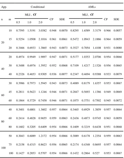
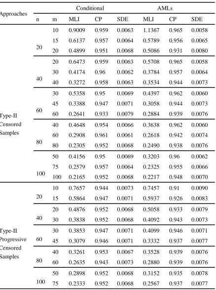
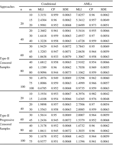
does not affect the calculations.

From the simulation results that reported in Tables 2 to 7, we can summarize the following main points:

1- It is worthwhile to note that for different values of



, the

CPs

are the same for the pivotal

z

₁ as expected because its distribution is independent from the

(8)

MLIs

will be the same for all the values of



as expected.

2- The values of

MLIs

_{generally decrease and the}

CPs

almost getting increase and the values of

SDEs

almost getting decrease as the sample size increases for

both parameters



and



. Moreover, the values of MLI for



and



generally increase with the same average of increasing the values of



and



respectively.

3- The values of MLI for



_and



_{based on the conditional inference are quite} shorter than those based on the AMLEs, in spite of they have almost higher

CPs

based on complete and type-II progressively censored samples. However, the

values of MLIs for



_{based on the AMLEs inference are almost shorter than} those based on the conditional inference when



=

0.5

and both approaches

have greater MLIs_{values for}

n

=

10

, based on type-II censored samples.

4- Both approaches are almost conservative for estimating



and



, however the AMLEs approach is anti-conservative when the sample size is less than or equal to 20.

5- Generally, the results based on the type-II progressive censored samples are better than those based on the type-II censored samples, in which they have shorter

MLIsand higher

CPs

.

6- _{Finally, both approaches are adequate because their}

SDEs

are less than



2%

for the nominal level

95%

.

Thus the simulation results indicated that the conditional intervals possess good statistical properties and they can perform quite well even when the sample size is extremly small. However, the AMLEs approach turns out to be impercise or even unreliable for small or highly type-II censored samples.

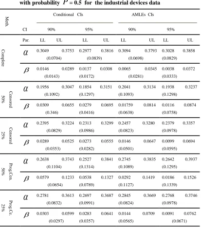
4. Numerical examples

Example 1:

Consider the data in Aarset (1987) that represent the lifetime of 50 industrial devices, which fit the Weibull extension model.

0.1, 0.2, 1, 1, 1, 1, 1, 2, 3, 6, 7, 11, 12, 18, 18, 18, 18, 18, 21, 32, 36, 40, 45, 46, 47, 50, 55, 60, 63, 63, 67, 67, 67, 67,72, 75, 79, 82, 82, 83, 84, 84, 84, 85, 85, 85, 85, 85, 86, 86.

Thus for purpose of comparison, the 90% and 95% confidence intervals for the

(9)



and



based on the conditional approach are shorter than those based on the AMLEs approach which ensure the simulation results.

Example 2:

Consider the data given in Chen (2000 ) and Wu et al. (2004) that represents 11 observations of a computer-generated sample of size n = 15 from the Weibull extension

model with parameters



=

0

.

02

and



=

0

.

5

:

0.29 , 1.44 , 8.38 , 8.66 , 10.20 , 11.04 , 13.44 , 14.37, 17.05 , 17.13 , 18.35.

It was found by Chen (2000) _{that the 95% confidence interval for the shape parameter}



is ( 0.19, 0.62 ) with interval length 0.43, based on a pivotal quantity for



. Wu et al. (2004) proposed a new pivotal quantity for the shape parameter and evaluated the 95% confidence interval for the shape parameter as ( 0.27, 0.60 ) with interval length 0.33 which is shorter than Chen (2000) interval. Thus for purpose of comparison the 95% conditional confidence interval for the shape parameter is ( 0.35, 0.59 ) with interval length 0.24 . Also the 95% AMLEs for the shape parameter is ( 0.37, 0.64 ) with interval length 0.27. Thus the conditional and the AMLEs confidence intervals are shorter than both Chen (2000) and Wu et al. (2004) intervals.

5. Conclusion

In this paper, a new application for the conditional inference has been applied to inference on the shape-scale family parameters with application to the Weibull extension model based on the generalized order statistics. Moreover, for purpose of comparison the asymptotic maximum likelihood estimates has been applied to measure the performances of the proposed approach based on the Monte Carlo simulations that indicated the conditional approach possess good statistical properties and can perform quite well even when the sample size is extremly small. However, the AMLEs turn out to be impercise or even unreliable for small or highly censored samples.

References

1. Aarset, M.V. (1987). How to identify bathtub hazard rate, IEEE trans. Rel. Vol. 36, No. 1, 106-108.

2. Chen, Z. (2000). A new two-parameter lifetime distribution with bathtub-shape or increasing failure rate function. Statistics & Probability Letters . Vol. 49, 155-161.

3. Fisher, R.A. (1934). Two New Properties of Mathematical Likelihood. Proc. R. Soc. A 144, 285-307.

4. Kamps, U. A. (1995). Concept of generalized order statistics. J. Statistical Planning & Inference, Vol. 48, 1-23.

(10)

6. Lawless, J.F. (1972). Confidence interval estimation for the parameters of the Weibull distribution. Utilitas Mathematica, Vol. 2, 71- 87.

7. Lawless, J.F. (1973). Conditional versus Unconditional Confidence Intervals for the Parameters of the Weibull Distribution. J.Amer.Statist. Assoc., Vol. 68, 669-679.

8. Lawless, J.F. (1974). Approximations to Confidence Intervals in the Extreme Value and Weibull Distributions. Biometrika, Vol. 61, 123-129.

9. Lawless, J.F. (1975). Construction of Tolerance bounds for the Extreme Value and Weibull Distributions. Technometrics, Vol. 71, 255-261.

10. Lawless, J.F. (1978). Confidence interval Estimation for the Weibull and Extreme value Distributions. Technometrics, Vol. 20, 355-364.

11. Lawless, J. F. (1980). Inference in the Generalized Gamma and log Gamma Distributions. Technometrics, Vol. 22, 3, 409-419.

12. Lawless, J.F. (1982). Statistical Models and Methods for Lifetime Data. John Wiley & Sons. New York.

13. Maswadah, M. (2003). Conditional Confidence Interval Estimation For The Inverse Weibull distribution Based on Censored Generalized Order Statistics. Journal of Statistical Computation and Simulation, Vol. 73, No. 12, 887-898.

14. Maswadah, M.(2005). Conditional Confidence Interval Estimation For The Type-II Extreme Value Distribution Based on Censored Generalized Order Statistics Journal of Applied Statistical Science, Vol. 14, No. 1/2, 71-84.

15. Pham, H. and Lai, Chin-Diew (2007). On recent generalizations of the Weibull distribution. IEEE Transaction on Reliability, Vol. 56, 454-458.

16. Silva, G.O., Ortega, E.M.M., and Cordeiro, G.M. (2009). A log-extended Weibull regression model. Computational Statistics and Data Analysis, Vol. 53, 4482-4489.

17. Tang, Y., Xie, M. and Goh, T.N. (2003). Statistical Analysis of the Weibull Extension Model. Comm. In Statist.-Theory and Methods, Vol. 32, No. 5, 913-928.

18. Wang, K.S., Hsu, F.S. and Liu, P.P. (2002). Modeling the bathtub shaped hazard rate function in terms of Reliability. Reliability Engineering and System Safety. Vol. 75, 397-406.

19. Wu, J., Lu, H., Chen, C. and Wu, C. (2004). Statistical Inference about shape parameter of the new two-parameter Bathtub-shaped lifetime distribution. Quality and Reliability Engineering International, Vol. 20, 607-616.

20. Xie, M., Lai, C.D. (1996).Reliability analysis using an additive Weibull model with bathtub-shaped failure rate function. Rliability Engineering & System Saftey. Vol. 52, No. 1, 87-93.

(11)

Table 2: The (MLIs), (CPs) and (SDEs) for the conditional and the AMLEs approaches when the nominal level is 95% for the parameter



with

5

.

0

=



to the complete and censored samples with censored levels (50%, 25% and 0.0%)

App. Conditional AMLs

n m

MLI ,



CP SDE

MLI ,



CP SDE

0.5 1.0 2.0 0.5 1.0 2.0

20

10 0.7595 1.5191 3.0382 0.948 0.0070 0.8295 1.6589 3.3179 0.966 0.0057

15 0.5254 1.0508 2.1016 0.961 0.0061 0.5472 1.0943 2.1886 0.964 0.0059

20 0.3466 0.6933 1.3865 0.943 0.0073 0.3527 0.7054 1.4108 0.931 0.0080

40

20 0.4974 0.9949 1.9897 0.947 0.0071 0.5177 1.0353 2.0706 0.954 0.0066

30 0.3488 0.6976 1.3952 0.952 0.0068 0.7109 1.4217 2.1326 0.956 0.0065

40 0.2326 0.4653 0.9305 0.936 0.0077 0.2347 0.4694 0.9388 0.933 0.0079

60

30 0.3986 0.7973 1.5945 0.943 0.0073 0.4089 0.8179 1.6357 0.953 0.0067

45 0.2811 0.5623 1.1246 0.946 0.0071 0.2847 0.5693 1.1386 0.949 0.0069

60 0.1864 0.3729 0.7458 0.946 0.0071 0.1875 0.3751 0.7502 0.945 0.0072

80

40 0.3401 0.6801 1.3602 0.957 0.0064 0.3465 0.6929 1.3859 0.957 0.0064

60 0.2414 0.4828 0.9655 0.959 0.0063 0.2436 0.4873 0.9745 0.963 0.0059

80 0.1602 0.3205 0.6409 0.954 0.0066 0.1609 0.3219 0.6438 0.951 0.0068

100

50 0.3043 0.6089 1.2172 0.954 0.0066 0.3089 0.6178 1.2354 0.959 0.0063

75 0.2158 0.4315 0.8623 0.956 0.0065 0.2174 0.4348 0.8695 0.957 0.0064

(12)

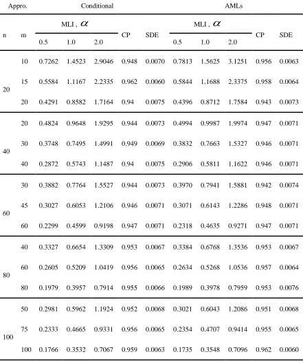
Table 3: The (MLIs), (CPs) and (SDEs) for the conditional and the AMLEs approaches when the nominal level is 95% for the parameter



with

2

=



to the complete and censored samples with censored levels (50%, 25% and 0.0%)

Appro. Conditional AMLs

n m

MLI ,



CP SDE

MLI ,



CP SDE

0.5 1.0 2.0 0.5 1.0 2.0

20

10 0.7262 1.4523 2.9046 0.948 0.0070 0.7813 1.5625 3.1251 0.956 0.0063

15 0.5584 1.1167 2.2335 0.962 0.0060 0.5844 1.1688 2.3375 0.958 0.0064

20 0.4291 0.8582 1.7164 0.94 0.0075 0.4396 0.8712 1.7584 0.943 0.0073

40

20 0.4824 0.9648 1.9295 0.944 0.0073 0.4994 0.9987 1.9974 0.947 0.0071

30 0.3748 0.7495 1.4991 0.949 0.0069 0.3832 0.7663 1.5327 0.946 0.0071

40 0.2872 0.5743 1.1487 0.94 0.0075 0.2906 0.5811 1.1622 0.946 0.0071

60

30 0.3882 0.7764 1.5527 0.944 0.0073 0.3970 0.7941 1.5881 0.942 0.0074

45 0.3027 0.6053 1.2106 0.946 0.0071 0.3071 0.6143 1.2286 0.948 0.0071

60 0.2299 0.4599 0.9198 0.947 0.0071 0.2318 0.4635 0.9271 0.947 0.0071

80

40 0.3327 0.6654 1.3309 0.953 0.0067 0.3384 0.6768 1.3536 0.953 0.0067

60 0.2605 0.5209 1.0419 0.956 0.0065 0.2634 0.5268 1.0536 0.957 0.0064

80 0.1979 0.3957 0.7914 0.955 0.0066 0.1989 0.3978 0.7959 0.953 0.0076

100

50 0.2981 0.5962 1.1924 0.952 0.0068 0.3021 0.6043 1.2086 0.951 0.0068

75 0.2333 0.4665 0.9331 0.956 0.0065 0.2354 0.4707 0.9414 0.955 0.0065

(13)

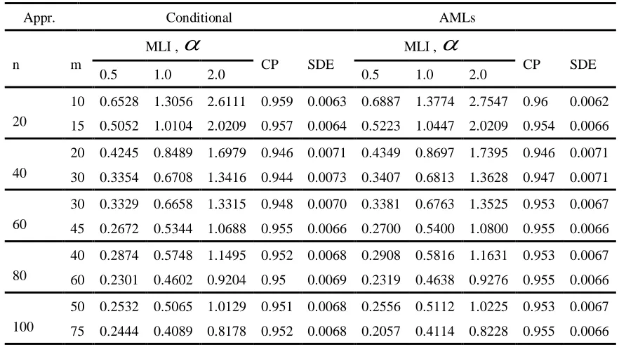
Table 4: The (MLIs), (CPs) and (SDEs) for the conditional and the AMLEs approaches when the nominal level is 95% for the parameter



with



=

0

.

5

to the progressive type-II censoring with binomal random removal with probability

P

= 0.5 and censored levels (50% and 75%)

_Appro. _Conditional _AMLs

n m

MLI ,



CP SDE

MLI ,



CP SDE

0.5 1.0 2.0 0.5 1.0 2.0

20

10 0.5310 1.0620 2.1241 0.956 0.0065 0.5512 1.1023 2.2046 0.945 0.0072

15 0.4092 0.8183 1.6366 0.952 0.0068 0.4189 0.8377 1.6754 0.943 0.0073

40

20 0.3434 0.6867 1.3735 0.947 0.0071 0.3493 0.6986 1.3973 0.934 0.0079

30 0.2717 0.5433 1.0867 0.941 0.0075 0.2748 0.5497 1.0993 0.937 0.0077

60

30 0.2697 0.5394 1.0789 0.953 0.0067 0.2729 0.5457 1.0914 0.952 0.0068

45 0.2167 0.4333 0.8666 0.955 0.0066 0.2183 0.4367 0.8734 0.956 0.0065

80

40 0.2328 0.4655 0.9311 0.953 0.0067 0.2348 0.4697 0.9394 0.945 0.0072

60 0.1864 0.3728 0.7457 0.948 0.0070 0.1875 0.3751 0.7501 0.947 0.0071

100

50 0.2048 0.4096 0.8192 0.951 0.0068 0.2062 0.4125 0.8249 0.951 0.0068

75 0.1653 0.3306 0.6613 0.946 0.0071 0.1661 0.3322 0.6644 0.95 0.0069

Table 5: The (MLIs), (CPs) and (SDEs) for the conditional and the AMLEs approaches when the nominal level is 95% for the parameter



_with



=

2

, to the progressive type-II censoring with binomal random removal with probability

P

= 0.5 and censored levels (50% and 75%)

Appr. Conditional AMLs

n m

MLI ,



CP SDE

MLI ,



CP SDE

0.5 1.0 2.0 0.5 1.0 2.0

20

10 0.6528 1.3056 2.6111 0.959 0.0063 0.6887 1.3774 2.7547 0.96 0.0062

15 0.5052 1.0104 2.0209 0.957 0.0064 0.5223 1.0447 2.0209 0.954 0.0066

40

20 0.4245 0.8489 1.6979 0.946 0.0071 0.4349 0.8697 1.7395 0.946 0.0071

30 0.3354 0.6708 1.3416 0.944 0.0073 0.3407 0.6813 1.3628 0.947 0.0071

60

30 0.3329 0.6658 1.3315 0.948 0.0070 0.3381 0.6763 1.3525 0.953 0.0067

45 0.2672 0.5344 1.0688 0.955 0.0066 0.2700 0.5400 1.0800 0.955 0.0066

80

40 0.2874 0.5748 1.1495 0.952 0.0068 0.2908 0.5816 1.1631 0.953 0.0067

60 0.2301 0.4602 0.9204 0.95 0.0069 0.2319 0.4638 0.9276 0.955 0.0066

100

50 0.2532 0.5065 1.0129 0.951 0.0068 0.2556 0.5112 1.0225 0.953 0.0067

(14)

Table 6: The conditional and the AMLEs (MLIs), (CPs) and (SDEs) based on the

nominal level 95% for the parameter



with



=

0

.

5

based on the type-II censored and type-II progressively censoring with binomal random removal

with probability

P

= 0.5 and censored levels (50%, 25% and 0.0%)

Approaches

Conditional AMLs

n m MLI CP SDE MLI CP SDE

Type-II

Censored Samples

20

10 0.9009 0.959 0.0063 1.1367 0.965 0.0058

15 0.6137 0.957 0.0064 0.5789 0.956 0.0065

20 0.4899 0.951 0.0068 0.5086 0.931 0.0080

40

20 0.6473 0.959 0.0063 0.5708 0.965 0.0058

30 0.4174 0.96 0.0062 0.3784 0.957 0.0064

40 0.3272 0.958 0.0063 0.3534 0.944 0.0073

60

30 0.5358 0.95 0.0069 0.4397 0.962 0.0060

45 0.3388 0.947 0.0071 0.3058 0.944 0.0073

60 0.2641 0.933 0.0079 0.2884 0.939 0.0076

80

40 0.4648 0.954 0.0066 0.3638 0.962 0.0060

60 0.2908 0.961 0.0061 0.2618 0.942 0.0074

80 0.2305 0.952 0.0068 0.2490 0.938 0.0076

100

50 0.4156 0.95 0.0069 0.3203 0.96 0.0062

75 0.2579 0.957 0.0064 0.2325 0.955 0.0066

100 0.2165 0.952 0.0068 0.2217 0.948 0.0070

Type-II Progressive Censored Samples

20

10 0.7657 0.944 0.0073 0.7457 0.91 0.0090

15 0.5864 0.947 0.0071 0.5937 0.926 0.0083

40

20 0.4876 0.952 0.0068 0.5058 0.933 0.0079

30 0.3838 0.952 0.0068 0.4092 0.943 0.0073

60

30 0.3853 0.947 0.0071 0.4099 0.946 0.0071

45 0.3079 0.946 0.0071 0.3332 0.937 0.0077

80

40 0.3261 0.953 0.0067 0.3528 0.939 0.0076

60 0.2635 0.943 0.0073 0.2880 0.939 0.0076

(15)

Table 7: The conditional and the AMLEs (MLIs), (CPs) and (SDEs) based on the nominal level 95% for the parameter



with



=

2

based on the type-II censored and type-type-II progressively censoring with binomal random removal with probability

P

= 0.5 and censored levels (50%, 25% and 0.0%)

Approaches Conditional AMLs

n m MLI CP SDE MLI CP SDE

Type-II Censored Samples

20

10 3.3151 0.959 0.0063 7.8257 0.96 0.0062

15 2.4304 0.96 0.0062 5.3412 0.957 0.0049

20 1.9981 0.952 0.0068 2.8499 0.973 0.0051

40

20 2.3602 0.961 0.0061 5.5416 0.955 0.0066

30 1.6418 0.959 0.0063 2.6937 0.97 0.0054

40 1.3228 0.958 0.0063 1.6728 0.959 0.0063

60

30 1.9429 0.945 0.0072 3.7843 0.95 0.0069

45 1.3283 0.947 0.0071 2.0638 0.964 0.0059

60 1.0638 0.933 0.0079 1.3067 0.958 0.0063

80

40 1.6812 0.958 0.0063 2.9102 0.954 0.0066

60 1.1389 0.96 0.0062 1.7038 0.969 0.0055

80 0.9096 0.944 0.0073 1.1062 0.959 0.0063

100

50 1.4976 0.949 0.0069 2.5298 0.962 0.0060

75 1.0086 0.959 0.0063 1.4999 0.966 0.0057

100 0.6785 0.952 0.0068 0.9735 0.959 0.0063

Type-II Progressive Censored Samples

20

10 3.1934 0.953 0.0067 6.3976 0.982 0.0042

15 2.4108 0.954 0.0066 3.6365 0.976 0.0048

40

20 1.9898 0.957 0.0063 2.7506 0.97 0.0054

30 1.5563 0.958 0.0063 2.0085 0.959 0.0063

60

30 1.5614 0.95 0.0069 2.0007 0.964 0.0059

45 1.2436 0.945 0.0072 1.5379 0.952 0.0068

80

40 1.3178 0.952 0.0068 1.6732 0.96 0.0062

60 1.0611 0.945 0.0072 1.3035 0.96 0.0062

100

50 1.1678 0.952 0.0068 1.4421 0.964 0.0059

(16)

Table 8: The Lower (LL) and the Upper limits (UL) and the lengths of the 90% and 95% confidence intervals (CI) for the parameters α, β based on the Conditional and the AMLEs approaches for complete, Type-II censored and Type-II progressive censored samples with binomial random removal with probability

P

= 0.5 for the industrial devices data

M

et

h.

CI

Conditional CIs

90% 95%

AMLEs CIs

90% 95%

C

om

p

le

te

Par. LL UL LL UL LL UL LL UL



0.3049 0.3753 (0.0704)

0.2977 0.3816 (0.0839)

0.3094 0.3793 (0.0698)

0.3028 0.3858 (0.0829)



0.0146 0.0289 (0.0143)

0.0137 0.0308 (0.0172)

0.0065 0.0345 (0.0281)

0.0038 0.0372 (0.0333)

C

ens

o

re

d

50%



0.1956 0.3047 (0.1092)

0.1854 0.3151 (0.1297)

0.2041 0.3134 (0.1093)

0.1938 0.3237 (0.1298)



0.0309 0.0655 (0.346)

0.0279 0.0695 (0.0416)

0.01759 0.0814 (0.0638)

0.0116 0.0874 (0.0758)

C

ens

o

re

d

25%



0.2395 0.3224 (0.0829)

0.2313 0.3299 (0.0986)

0.2457 0.3280 (0.0823)

0.2379 0.3357 (0.0978)



0.0289 0.0525 (0.0353)

0.0273 0.0555 (0.0282)

0.0146 0.0647 (0.0501)

0.0099 0.0694 (0.0595)

P

rog

,C

en

.

50%



0.2638 0.3743 (0.1104)

0.2527 0.3841 (0.1314)

0.2745 0.3835 (0.1089)

0.2642 0.3937 (0.1295)



0.0579 0.1233 (0.0654)

0.0538 0.1327 (0.0789)

0.0292 0.1419 (0.1127)

0.0186 0.1526 (0.1339)

P

rog

.C

e.

25%



0.2781 0.3613 (0.0832)

0.2697 0.3687 (0.0991)

0.2845 0.3669 (0.0824)

0.2768 0.3746 (0.0978)



0.0303 0.0599 (0.0297)

0.0283 0.0641 (0.0357)

0.0144 0.0709 (0.0565)

0.0091 0.0762 (0.0671)