Transmuted New Generalized Inverse Weibull Distribution

Transmuted New Generalized Inverse Weibull Distribution

Muhammad Shuaib Khan

School of Mathematical and Physical Sciences

The University of Newcastle, Callaghan, NSW 2308, Australia shuaib.stat@gmail.com

Robert King

School of Mathematical and Physical Sciences

The University of Newcastle, Callaghan, NSW 2308, Australia robert.king@newcastle.edu.au

Irene Lena Hudson

School of Mathematical and Physical Sciences

The University of Newcastle, Callaghan, NSW 2308, Australia irene.Hudson@newcastle.edu.au

Abstract

This paper introduces the transmuted new generalized inverse Weibull distribution by using the quadratic rank transmutation map (QRTM) scheme studied by Shaw et al. (2007). The proposed model contains twenty three lifetime distributions as special sub-models. Some mathematical properties of the new distribution are formulated, such as quantile function, Rényi entropy, mean deviations, moments, moment generating function and order statistics. The method of maximum likelihood is used for estimating the model parameters. We illustrate the flexibility and potential usefulness of the new distribution by means of two real data sets.

Keywords: New generalized inverse Weibull distribution; Moment estimation; Moment generating function; Order statistics; Maximum likelihood estimation.

1. Introduction

The cdf of the NGIW distribution is given by

𝐹(𝑥) = 1 −⁡[1 − 𝑒𝑥𝑝⁡{−𝛼 𝑥− 𝛾 (

1 𝑥)

𝛽 }]

𝜙

,⁡⁡⁡⁡⁡⁡⁡⁡⁡⁡⁡⁡⁡⁡⁡⁡⁡⁡⁡⁡⁡⁡⁡⁡⁡⁡⁡⁡⁡⁡⁡⁡⁡⁡⁡⁡⁡⁡⁡⁡⁡⁡⁡⁡⁡⁡⁡⁡⁡⁡⁡⁡⁡⁡⁡⁡⁡⁡⁡⁡⁡⁡⁡⁡⁡⁡⁡⁡⁡⁡⁡⁡⁡⁡(1)

where⁡𝛽, 𝜙 > 0 are the shape parameters and 𝛼, 𝛾 > 0 are the scale parameters. The probability density function corresponding to (1) is given by

𝑓(𝑥) = 𝜙 {𝛼 + 𝛽𝛾 (1 𝑥)

𝛽−1 } (1

𝑥) 2

𝑒𝑥𝑝 {−𝛼 𝑥− 𝛾 (

1 𝑥)

𝛽 } [1

− 𝑒𝑥𝑝 {−𝛼 𝑥− 𝛾 (

1 𝑥)

𝛽 }]

𝜙−1

,⁡⁡⁡⁡⁡⁡⁡⁡⁡⁡⁡⁡⁡⁡⁡⁡⁡⁡⁡⁡⁡⁡⁡⁡⁡⁡⁡⁡⁡⁡⁡⁡⁡⁡⁡⁡⁡⁡⁡⁡⁡⁡⁡⁡⁡⁡⁡⁡⁡⁡⁡⁡⁡⁡⁡⁡⁡⁡⁡⁡⁡⁡⁡⁡⁡⁡⁡⁡⁡(2)

The CDF given in equation (1) approches to the eleven lifetime distributions when its parameters change. Khan and King (2012) proposed the modified Inverse Weibull distribution and presented a comprehensive description of the mathematical properties of this model along with its reliability behavior. Using quadratic rank transmutation map (QRTM) technique, we introduce the transmuted the new generalized inverse Weibull (NGIW) distribution by introducing a new parameter λ that would offer more flexibility in the proposed model. Several distributions have been proposed under this methodology such as transmuted extreme value distribution (Gokarna and Chris, 2009) studied with application to climate data, the transmuted Weibull distribution (Gokarna and Chris, 2011) proposed with two applications, Gokarna (2013) proposed the transmuted Log-Logistic distribution and studied its various structural properties. Khan and King (2013) proposed the transmuted modified Weibull distribution as an important competitive model with eleven lifetime distributions as sub-models along with its theoretical properties. Khan and King (2013) studied the flexibility of the transmuted generalized Inverse Weibull distribution with application to reliability data. Merovci (2013) studied the transmuted rayleigh distribution. Elbatal et al. (2013a, 2013b) proposed and studied the transmuted additive Weibull and transmuted modified inverse Weibull distributions. Khan et al. (2014a, 2014b) proposed the transmuted inverse Weibull distribution and studied its various structural properties with an application to survival data. More recently, Khan and King (2015) explored the flexibility of the transmuted modified Inverse Rayleigh distribution using QRTM technique which extends the modified Inverse Rayleigh distribution with application to reliability data. A random variable X is said to have transmuted distribution if its cumulative distribution function (cdf) is given by

𝐹(𝑥) = (1 + 𝜆)𝐺(𝑥) − 𝜆𝐺(𝑥)2_{, ⁡⁡⁡⁡⁡⁡⁡⁡⁡⁡⁡⁡|𝜆| ≤ 1⁡⁡⁡⁡⁡⁡⁡⁡⁡⁡⁡⁡⁡⁡⁡⁡⁡⁡⁡⁡⁡⁡⁡⁡⁡⁡ (3)} and

𝑓(𝑥) = 𝑔(𝑥){(1 + 𝜆) − 2𝜆𝐺(𝑥)},⁡⁡⁡⁡⁡⁡⁡⁡⁡⁡⁡⁡⁡⁡⁡⁡⁡⁡⁡⁡⁡⁡⁡⁡⁡⁡⁡⁡⁡⁡⁡⁡⁡⁡⁡⁡⁡⁡⁡⁡⁡⁡⁡⁡⁡⁡⁡⁡⁡⁡⁡⁡ (4) where 𝐺(𝑥) is the cdf of the baseline distribution. It is important to note that at λ = 0 we have the distribution of the baseline random variable.

entropy and mean deviations in section 5. The order statistics are formulated in Section 6. In Section 7, we compare the proposed model with three other lifetime distributions by means of two real data sets to illustrate its usefulness. In Section 8, we offer some Concluding remarks.

2. Transmuted New Generalized Inverse Weibull Distribution

A random variable 𝑿 is said to have transmuted new generalized inverse Weibull (TNGIW) distribution with parameters ⁡𝜶, 𝜷, 𝜸, 𝝓 > 𝟎 and |𝛌| ≤ 𝟏, 𝒙 > 𝟎. If the probability density function is given by

𝑓(𝑥) = ϕ {α + βγ (1 𝑥)

𝛽−1

} exp {−α 𝑥− 𝛾 (

1 𝑥)

𝛽 } [1

− exp {−α 𝑥− 𝛾 (

1 𝑥)

𝛽 }]

ϕ−1

𝒰(𝑥),⁡⁡⁡⁡⁡⁡⁡(5)

𝒰(𝑥) = (1 𝑥)

2

{1 − λ + 2λ [1 − exp⁡{−α 𝑥− 𝛾 (

1 𝑥)

𝛽 }]

ϕ

}.⁡⁡⁡⁡⁡⁡⁡⁡⁡⁡⁡⁡⁡⁡⁡⁡⁡⁡⁡⁡⁡⁡⁡⁡⁡⁡⁡⁡⁡⁡⁡⁡⁡⁡⁡⁡⁡⁡⁡⁡⁡⁡⁡⁡⁡⁡⁡⁡(6)

The CDF corresponding to equation (5) is given by

𝐹(𝑥) = {1 − [1 − exp⁡{−α 𝑥− 𝛾 (

1 𝑥)

𝛽 }]

ϕ

} {1

+ λ [1 − exp⁡{−α 𝑥− 𝛾 (

1 𝑥)

𝛽 }]

ϕ

}.⁡⁡⁡⁡⁡⁡⁡⁡⁡⁡⁡⁡⁡⁡⁡⁡⁡⁡⁡⁡⁡⁡⁡⁡⁡⁡⁡⁡⁡⁡⁡⁡⁡⁡⁡⁡⁡⁡⁡⁡⁡⁡⁡⁡⁡⁡⁡⁡⁡⁡⁡⁡⁡⁡⁡⁡⁡⁡⁡⁡⁡⁡⁡(7)

Figure 1 shows the visualizations of the transmuted new generalized inverse Weibull PDF with some selected choice of parameters. Some useful characterizations of the TNGIW distribution are formulated as reliability function (RF), hazard function and reversed hazard function defined as

𝑅(𝑥) = 1 − {1 − [1 − exp {−α 𝑥− 𝛾 (

1 𝑥)

𝛽 }]

ϕ

} {1

+ λ [1 − exp {−α 𝑥− 𝛾 (

1 𝑥)

𝛽 }]

ϕ

},⁡⁡⁡⁡⁡⁡⁡⁡⁡⁡⁡⁡⁡⁡⁡⁡⁡⁡⁡⁡⁡⁡⁡⁡⁡⁡⁡⁡⁡⁡⁡⁡⁡⁡⁡⁡⁡⁡⁡⁡⁡⁡⁡⁡⁡⁡⁡⁡⁡⁡⁡⁡⁡⁡⁡⁡⁡⁡⁡⁡⁡⁡⁡(8)

ℎ(𝑥)

=

ϕ (α + βγ (1 𝑥)

𝛽−1

) exp {−α 𝑥− 𝛾 (

1 𝑥)

𝛽

} [1 − exp {−α 𝑥− 𝛾 (

1 𝑥)

𝛽 }]

ϕ−1 𝒰(𝑥)

1 − {1 − [1 − exp⁡{−α 𝑥− 𝛾 (

1 𝑥)

𝛽 }]

ϕ

} {1 + λ [1 − exp⁡{−α 𝑥− 𝛾 (

1 𝑥)

𝛽 }]

ϕ }⁡⁡⁡⁡⁡⁡

,⁡⁡⁡⁡⁡(9)

and

𝑟(𝑥)

=

ϕ (α + βγ (1 𝑥)

𝛽−1

) exp {−α 𝑥− 𝛾 (

1 𝑥)

𝛽

} [1 − exp {−α 𝑥− 𝛾 (

1 𝑥)

𝛽 }]

ϕ−1 𝒰(𝑥)

{1 − [1 − exp⁡{−α 𝑥− 𝛾 (

1 𝑥)

𝛽 }]

ϕ

} {1 + λ [1 − exp⁡{−α 𝑥− 𝛾 (

1 𝑥)

𝛽 }]

ϕ }⁡⁡⁡⁡⁡⁡

Figure 1: Plots of the TNGIW pdf for some parameter values.

Figure 2: Plots of the TNGIW hf for some parameter values.

0.5 1.0 1.5 2.0 2.5 3.0 3.5 4.0

0

.0

0

.5

1

.0

1

.5

1, 1.5

x

f(x)

3, 2, 1 1, 1.5, 0.5 2, 3, 0.1 2.5, 4, 0.5

4, 5, 1

0.5 1.0 1.5 2.0 2.5 3.0

0

.0

0

.5

1

.0

1

.5

2

.0

0.5, 1.5, 3

x

f(x)

3, 1 1, 0.5 2, 0.1 2.5, 0.5 5, 1

0.5 1.0 1.5 2.0 2.5 3.0

0

.0

0

.5

1

.0

1

.5

1, 3, 2, 3

x

f(x)

1 0.5 0.1 0.5 1

0.5 1.0 1.5 2.0 2.5 3.0

0

.0

0

.5

1

.0

1

.5

0.3, 2, 1

x

f(x)

1, 3 2, 1 2.5, 2 2.5, 3 3, 3

0.5 1.0 1.5 2.0 2.5 3.0 3.5 4.0

0

1

2

3

1, 1.5

x

h

(x)

3, 2, 1

1, 1.5, 0.5 2, 3, 0.1

2.5, 4, 0.5

4, 5, 1

0.5 1.0 1.5 2.0 2.5 3.0

0

1

2

3

4

0.3, 2, 1

x

h

(x)

The cumulative hazard function (CHF) of the TNGIW distribution is defined as

𝐻(𝑥)

= ∫

ϕ (α + βγ (1 𝑥)

𝛽−1

) exp {−α 𝑥− 𝛾 (

1 𝑥)

𝛽

} [1 − exp {−α 𝑥− 𝛾 (

1 𝑥)

𝛽 }]

ϕ−1 𝒰(𝑥)

1 − {1 − [1 − exp⁡{−α 𝑥− 𝛾 (

1 𝑥)

𝛽 }]

ϕ

} {1 + λ [1 − exp⁡{−α 𝑥− 𝛾 (

1 𝑥)

𝛽 }]

ϕ }⁡⁡⁡⁡⁡

d𝑥, 𝑥

0

𝐻(𝑥) = −ln [1

− {1 − [1 − exp {−α 𝑥− 𝛾 (

1 𝑥)

𝛽 }]

ϕ

} {1

+ λ [1 − exp {−α 𝑥− 𝛾 (

1 𝑥)

𝛽 }]

ϕ

}].⁡⁡⁡⁡⁡⁡⁡⁡⁡⁡⁡⁡⁡⁡⁡⁡⁡⁡⁡⁡⁡⁡⁡⁡⁡⁡⁡⁡⁡⁡⁡⁡⁡⁡⁡⁡⁡⁡⁡⁡⁡⁡⁡⁡⁡⁡⁡⁡⁡⁡⁡⁡⁡⁡⁡⁡⁡⁡⁡(11)

The quantile function of the TNGIW distribution is the real solution of the following equation

𝛾 (1 𝑥𝑞)

𝛽 + 𝛼

𝑥𝑞+ 𝑙𝑛 {1 − (1 −

(1+𝜆)−√(1+𝜆)2_−4𝜆𝑞

2𝜆 )

1 𝜙

} = 0. (12)

A random variable 𝑋 with density (5) is denoted by 𝑋~𝑇𝑁𝐺𝐼𝑊(𝑥; 𝛼, 𝛽, 𝛾, 𝜙, 𝜆). When the transmuting parameter 𝜆 = 0, we obtain the new generalized inverse Weibull distribution. Figure 2 illustrates the hazard function of the TNGIW distribution with different choice of parameters. These visualizations of the failure rates show that the proposed model has upside down hazard rate function for some selected choice of parameters. Table 1 listed twenty three lifetime distributions as special sub-models of the transmuted new generalized inverse Weibull distribution.

Table 1: Sub-models of the Transmuted New Generalized Inverse Weibull distribution

S. No Model α β γ ϕ λ Authors

1 TNGIE − 1 − − − New

2 TNGIR − 2 − − − New

3 TMIW − − − 1 − Elbatal (2013b)

4 TMIR − 2 − 1 − Khan & King (2015)

5 TMIE − 1 − 1 − New

6 TGIW 0 − − − − Khan & King (2013b)

7 TGIR 0 2 − − − New

8 TGIE 0 1 − − − New

9 10 11

TIW TIR TIE

0 0 0

− 2 1

− − −

1 1 1

− − −

12 13 14 15 16 17 18 19 20 21 22 23

NGIW NGIR NGIE MIW MIR MIE GIW GIR GIE IW IR IE

− − − 0 0 0 0 0 0 − − −

− 2 1 − 2 1 − 2 1 − 2 1

− − − − − − − − − − − −

− − − 1 1 1 − − − 1 1 1

0 0 0 0 0 0 0 0 0 0 0 0

Khan & King (2016) New

New

Khan & King (2012) Khan M. S. (2014) New

Gusmão et al. (2009) Gusmão et al. (2009) Gusmão et al. (2009) Khan et al. (2008) Voda, V. Gh. (1972) Klugman et al. (2012)

Note: T: Transmuted; G, Generalized; M, Modified; N, New; I, Inverse; W, Weibull; E, Exponential; R, Rayleigh.

3. Statistical Properties

This section formulates the 𝑘𝑡ℎ moment and the moment generating function of the transmuted new generalized inverse Weibull distribution.

Theorem 1: If 𝑋⁡has the 𝑇𝑁𝐺𝐼𝑊(𝑥; 𝛼, 𝛽, 𝛾, 𝜙, 𝜆) distribution with |λ| ≤ 1, then the 𝑘𝑡ℎ moment of 𝑋 say 𝜇́𝑘 is given as follows

𝜇́_𝑘 = (1 − 𝜆) ∑ (𝜙 − 1

𝒾 )

∞

𝒾,𝒿=0

𝛾𝒿𝜙(−1)𝒾+𝒿(𝒾 + 1)𝒿

𝒿! 𝜉(𝛼, 𝛽, 𝛾, 𝒾, 𝒿, 𝑘)⁡⁡⁡⁡⁡⁡⁡⁡⁡⁡⁡⁡⁡⁡⁡⁡⁡⁡⁡

+2𝜆 ∑ (2𝜙 − 1

𝒾 )

∞

𝒾,𝒿=0

𝛾𝒿_𝜙(−1)𝒾+𝒿_{(𝒾 + 1)}𝒿

𝒿! 𝜉(𝛼, 𝛽, 𝛾, 𝒾, 𝒿, 𝑘),⁡⁡⁡

where

𝜉(𝛼, 𝛽, 𝛾, 𝒾, 𝒿, 𝑘) = 𝛼𝛤(𝛽𝒿 − 𝑘 + 1) (𝛼(𝒾 + 1))𝛽𝒿−𝑘+1

+𝛽𝛾𝛤(𝛽(𝒿 + 1) − 𝑘) (𝛼(𝒾 + 1))𝛽(𝒿+1)−𝑘 .

Proof: The 𝑘𝑡ℎ_{⁡moment of 𝑋 can be obtained from (5) as}

𝜇́_𝑘 = ∫ 𝑥𝑘 ∞

0

𝜙 (𝛼

+ 𝛽𝛾 (1 𝑥)

𝛽−1

) 𝑒𝑥𝑝 {−𝛼 𝑥− 𝛾 (

1 𝑥)

𝛽 } [1

− 𝑒𝑥𝑝 {−𝛼 𝑥− 𝛾 (

1 𝑥)

𝛽 }]

𝜙−1

𝒰(𝑥)𝑑𝑥,

By using equation (6) we can write the above integral as

(1 − 𝜆) ∫ 𝑥∞ 𝑘−2_{𝜙 (𝛼} 0

+ 𝛽𝛾 (1 𝑥) 𝛽−1 ) 𝑒𝑥𝑝 {−𝛼 𝑥− 𝛾 ( 1 𝑥) 𝛽

} [1 − 𝑒𝑥𝑝 {−𝛼 𝑥− 𝛾 ( 1 𝑥) 𝛽 }] 𝜙−1 𝑑𝑥

+2𝜆 ∫ 𝑥𝑘−2𝜙 (𝛼 ∞

0

+ 𝛽𝛾 (1 𝑥) 𝛽−1 ) 𝑒𝑥𝑝⁡{−𝛼 𝑥− 𝛾 ( 1 𝑥) 𝛽

} [1 − 𝑒𝑥𝑝 {−𝛼 𝑥− 𝛾 ( 1 𝑥) 𝛽 }] 2𝜙−1 𝑑𝑥,

the above integral reduces to

𝜇́_𝑘 = (1 − 𝜆) ∫ 𝑥𝑘−2𝜙𝛼 𝑒𝑥𝑝 {−𝛼 𝑥− 𝛾 (

1 𝑥)

𝛽

} [1 − 𝑒𝑥𝑝 {−𝛼 𝑥− 𝛾 ( 1 𝑥) 𝛽 }] 𝜙−1 𝑑𝑥 ∞ 0 +

⁡⁡⁡⁡⁡⁡⁡⁡⁡⁡(1 − 𝜆) ∫ 𝑥𝑘−𝛽−1_{𝜙𝛽𝛾 𝑒𝑥𝑝 {−}𝛼 𝑥− 𝛾 (

1 𝑥)

𝛽

} [1 − 𝑒𝑥𝑝 {−𝛼 𝑥− 𝛾 ( 1 𝑥) 𝛽 }] 𝜙−1 𝑑𝑥 ∞ 0

⁡⁡⁡⁡⁡⁡⁡⁡⁡⁡⁡⁡⁡+2𝜆 ∫ 𝑥𝑘−2_{𝜙𝛼⁡𝑒𝑥𝑝⁡{−}𝛼 𝑥− 𝛾 (

1 𝑥)

𝛽

} [1 − 𝑒𝑥𝑝⁡{−𝛼 𝑥− 𝛾 ( 1 𝑥) 𝛽 }] 2𝜙−1 𝑑𝑥 ∞ 0

⁡⁡⁡⁡⁡⁡⁡⁡⁡⁡⁡⁡⁡+2𝜆 ∫ 𝑥𝑘−𝛽−1_{𝜙𝛽𝛾𝑒𝑥𝑝⁡{−}𝛼 𝑥− 𝛾 (

1 𝑥)

𝛽

} [1 − 𝑒𝑥𝑝⁡{−𝛼 𝑥− 𝛾 ( 1 𝑥) 𝛽 }] 2𝜙−1 𝑑𝑥 ∞ 0 ,

By using the Binomial expansion, the above integral reduces to

𝜇́𝑘 = (1 − 𝜆) ∑ (𝜙 − 1_𝒾 ) ∞

𝒾=0

𝜙𝛼(−1)𝒾⁡⁡⁡∫ 𝑥𝑘−2𝑒𝑥𝑝 {−𝛼

𝑥(𝒾 + 1) − 𝛾 ( 1 𝑥)

𝛽

(𝒾 + 1)} 𝑑𝑥 ∞

0

⁡⁡⁡⁡⁡⁡⁡⁡+(1 − 𝜆) ∑ (𝜙 − 1

𝒾 )

∞

𝒾=0

𝜙𝛽𝛾(−1)𝒾⁡⁡⁡∫ 𝑥𝑘−𝛽−1𝑒𝑥𝑝 {−𝛼

𝑥(𝒾 + 1) ∞

0

− 𝛾 (1 𝑥)

𝛽

(𝒾 + 1)} 𝑑𝑥

⁡⁡⁡⁡⁡⁡⁡⁡+2𝜆 ∑ (2𝜙 − 1

𝒾 )

∞

𝒾=0

𝜙𝛼(−1)𝒾_{⁡∫ 𝑥}𝑘−2_{𝑒𝑥𝑝 {−}𝛼

𝑥(𝒾 + 1) − 𝛾 ( 1 𝑥)

𝛽

(𝒾 + 1)} 𝑑𝑥 ∞

0

⁡⁡

⁡⁡⁡⁡⁡⁡⁡⁡⁡+2𝜆 ∑ (2𝜙 − 1

𝒾 )

∞

𝒾=0

𝜙𝛽𝛾(−1)𝒾⁡⁡⁡∫ 𝑥𝑘−𝛽−1𝑒𝑥𝑝 {−𝛼

𝑥(𝒾 + 1) − 𝛾 ( 1 𝑥)

𝛽

(𝒾 + 1)} 𝑑𝑥, ∞

0

Hence, we obtain the final result

𝜇́_𝑘 = (1 − 𝜆) ∑ (𝜙 − 1

𝒾 )

∞

𝒾,𝒿=0

𝛾𝒿_𝜙(−1)𝒾+𝒿_{(𝒾 + 1)}𝒿

𝒿! 𝜉(𝛼, 𝛽, 𝛾, 𝒾, 𝒿, 𝑘)⁡⁡⁡⁡⁡⁡⁡⁡⁡⁡⁡⁡⁡⁡⁡⁡⁡⁡⁡

+2𝜆 ∑ (2𝜙 − 1

𝒾 )

∞

𝒾,𝒿=0

𝛾𝒿𝜙(−1)𝒾+𝒿(𝒾 + 1)𝒿

Theorem 2: If 𝑋⁡has the 𝑇𝑁𝐺𝐼𝑊(𝑥; 𝛼, 𝛽, 𝛾, 𝜙, 𝜆) distribution with |λ| ≤ 1, then the moment generating function of X say 𝑀_𝑥(𝑡) is given as follows

𝑀_𝑥(𝑡) = (1 − 𝜆) ∑ ∑ (𝜙 − 1

𝓃 )

∞

𝓃,ℓ=0

𝛾ℓ_𝜙(−1)𝓃+ℓ_{(𝓃 + 1)}ℓ_{{𝛼(𝓃 + 1)𝑡}}𝓂

ℓ! 𝓂! 𝜚(𝓃, ℓ, 𝓂)

∞

𝓂=0

⁡⁡⁡⁡

+2𝜆 ∑ ∑ (2𝜙 − 1

𝓃 )

∞

𝓃,ℓ=0

𝛾ℓ𝜙(−1)𝓃+ℓ(𝓃 + 1)ℓ_{{𝛼(𝓃 + 1)𝑡}}𝓂

ℓ! 𝓂! 𝜚(𝓃, ℓ, 𝓂)

∞

𝓂=0

,⁡⁡

where

𝜚(𝓃, ℓ, 𝓂) =𝛼𝛤(𝛽ℓ − 𝓂 + 1) (𝛼(𝓃 + 1))𝛽ℓ+1

+𝛽𝛾𝛤(𝛽(ℓ + 1) − 𝓂) (𝛼(𝓃 + 1))𝛽(ℓ+1)

.

Proof: By definition the⁡moment generating function of 𝑋 can be obtained from (5) as

𝑀𝑥(𝑡) =

∫ 𝑒𝑡𝑥 ∞

0

𝜙 (𝛼 + 𝛽𝛾 (1 𝑥)

𝛽−1

) 𝑒𝑥𝑝 {−𝛼 𝑥− 𝛾 (

1 𝑥)

𝛽

} [1 − 𝑒𝑥𝑝 {−𝛼 𝑥− 𝛾 (

1 𝑥)

𝛽 }]

𝜙−1

𝒰(𝑥)𝑑𝑥,

By using equation (6) the above integral reduces to

𝑀_𝑥(𝑡) = (1 − 𝜆) ∫ (1 𝑥)

2

𝜙𝛼 𝑒𝑥𝑝 {𝑡𝑥 −𝛼 𝑥− 𝛾 (

1 𝑥)

𝛽

} [1 − 𝑒𝑥𝑝 {−𝛼 𝑥− 𝛾 (

1 𝑥)

𝛽 }]

𝜙−1

𝑑𝑥 ∞

0

⁡⁡⁡⁡⁡⁡⁡⁡⁡⁡⁡⁡⁡⁡⁡⁡+(1 − 𝜆) ∫ (1 𝑥)

𝛽+1

𝜙𝛽𝛾 𝑒𝑥𝑝 {𝑡𝑥 −𝛼 𝑥− 𝛾 (

1 𝑥)

𝛽 } [1 ∞

0

− 𝑒𝑥𝑝 {−𝛼 𝑥− 𝛾 (

1 𝑥)

𝛽 }]

𝜙−1

𝑑𝑥

+2𝜆 ∫ (1 𝑥)

2

𝜙𝛼⁡𝑒𝑥𝑝⁡{𝑡𝑥 −𝛼 𝑥− 𝛾 (

1 𝑥)

𝛽

} [1 − 𝑒𝑥𝑝⁡{−𝛼 𝑥− 𝛾 (

1 𝑥)

𝛽 }]

2𝜙−1

𝑑𝑥 ∞

0

+2𝜆 ∫ (1 𝑥)

𝛽+1

𝜙𝛽𝛾𝑒𝑥𝑝⁡{𝑡𝑥 −𝛼 𝑥− 𝛾 (

1 𝑥)

𝛽

} [1 − 𝑒𝑥𝑝⁡{−𝛼 𝑥− 𝛾 (

1 𝑥)

𝛽 }]

2𝜙−1

𝑑𝑥, ∞

0

Finally we obtain the moment generating function of the TNGIW distribution as

𝑀_𝑥(𝑡) = (1 − 𝜆) ∑ ∑ (𝜙 − 1

𝓃 )

∞

𝓃,ℓ=0

𝛾ℓ𝜙(−1)𝓃+ℓ(𝓃 + 1)ℓ_{{𝛼(𝓃 + 1)𝑡}}𝓂

ℓ! 𝓂! 𝜚(𝓃, ℓ, 𝓂)

∞

𝓂=0

⁡⁡⁡⁡

+2𝜆 ∑ ∑ (2𝜙 − 1

𝓃 )

∞

𝓃,ℓ=0

𝛾ℓ𝜙(−1)𝓃+ℓ(𝓃 + 1)ℓ_{{𝛼(𝓃 + 1)𝑡}}𝓂

ℓ! 𝓂! 𝜚(𝓃, ℓ, 𝓂)

∞

𝓂=0

4. Maximum Likelihood Estimation

Consider the random samples 𝑥_1⁡, 𝑥₂, … , 𝑥_𝑛 consisting of 𝑛 observations from the

TNGIW(𝑥; 𝛼, 𝛽, 𝛾, 𝜙, 𝜆) distribution. The log-likelihood function ℒ = lnL of the density (5) for the parameter vector Θ = (𝛼, 𝛽, 𝛾, 𝜙, 𝜆) is given by

ℒ = 𝑛𝑙𝑛𝜙 + ∑ 𝑙𝑛 {𝛼 + 𝛽𝛾 (1 𝑥_𝑖) 𝛽−1 } 𝑛 𝑖=1 − ∑ (𝛼 𝑥_𝑖) 𝑛 𝑖=1

+ (𝜙 − 1) ∑ 𝑙𝑛 [1 − 𝑒𝑥𝑝⁡{−𝛼 𝑥_𝑖− 𝛾 ( 1 𝑥_𝑖) 𝛽 }] 𝑛 𝑖=1

+ ∑ 𝑙𝑛 (1 𝑥_𝑖)

2 𝑛

𝑖=1

− 𝛾 ∑ (1 𝑥_𝑖)

𝛽 𝑛

𝑖=1

+ ∑ 𝑙𝑛 {1 − 𝜆 + 2𝜆 [1 − 𝑒𝑥𝑝⁡{−𝛼 𝑥_𝑖 − 𝛾 ( 1 𝑥_𝑖) 𝛽 }] 𝜙 } 𝑛 𝑖=1 ⁡.⁡⁡⁡(15)

The components of score vector can be obtained by differentiating (15) with respect to

𝛼, 𝛽, 𝛾, 𝜙 and λ then equating it to zero, we obtain the estimating equations are

𝜕ℒ 𝜕𝛼= ∑ {𝛼 + 𝛽𝛾 ( 1 𝑥_𝑖) 𝛽−1 } −1

− ∑ (1 𝑥_𝑖) 𝑛

𝑖=1 𝑛

𝑖=1

+ (𝜙 − 1) ∑ 1 𝑥𝑖𝑒𝑥𝑝⁡{− 𝛼 𝑥𝑖− 𝛾 ( 1 𝑥𝑖) 𝛽 }

[1 − 𝑒𝑥𝑝⁡{−𝛼 𝑥𝑖− 𝛾 ( 1 𝑥𝑖) 𝛽 }] 𝑛 𝑖=1 + ∑ 2𝜆𝜙

𝑥𝑖[1 − 𝑒𝑥𝑝⁡{−

𝛼 𝑥𝑖− 𝛾 ( 1 𝑥𝑖) 𝛽 }] 𝜙−1 𝑒𝑥𝑝⁡{−𝛼 𝑥𝑖− 𝛾 ( 1 𝑥𝑖) 𝛽 }

{1 − 𝜆 + 2𝜆 [1 − 𝑒𝑥𝑝⁡{−𝛼 𝑥𝑖− 𝛾 ( 1 𝑥𝑖) 𝛽 }] 𝜙 } , 𝑛 𝑖=1 ⁡⁡⁡⁡⁡⁡⁡⁡⁡⁡⁡ 𝜕ℒ 𝜕𝛽= ∑

𝛾 (1 𝑥𝑖)

𝛽−1

[𝛽𝑙𝑛 (1 𝑥𝑖) + 1]

{𝛼 + 𝛽𝛾 (1 𝑥𝑖)

𝛽−1 } 𝑛

𝑖=1

+ (𝜙 − 1) ∑ 𝛾 (1

𝑥𝑖)

𝛽 𝑙𝑛 (1

𝑥𝑖) 𝑒𝑥𝑝⁡{− 𝛼 𝑥𝑖− 𝛾 ( 1 𝑥𝑖) 𝛽 }

[1 − 𝑒𝑥𝑝⁡{−𝛼 𝑥𝑖− 𝛾 ( 1 𝑥𝑖) 𝛽 }] 𝑛 𝑖=1

−𝛾 ∑ (1 𝑥𝑖 )

𝛽 𝑙𝑛 (1

𝑥𝑖 ) 𝑛 𝑖=1 + ∑ 2𝜆𝛾 𝜙

𝑥𝑖𝛽[1 − 𝑒𝑥𝑝⁡{−

𝛼 𝑥𝑖− 𝛾 ( 1 𝑥𝑖) 𝛽 }] 𝜙−1 𝑒𝑥𝑝⁡{−𝛼 𝑥𝑖− 𝛾 ( 1 𝑥𝑖) 𝛽 }

[𝑙𝑛 (1 𝑥𝑖)]

−1

{1 − 𝜆 + 2𝜆 [1 − 𝑒𝑥𝑝⁡{−𝛼 𝑥𝑖− 𝛾 ( 1 𝑥𝑖) 𝛽 }] 𝜙 } , 𝑛 𝑖=1 𝜕ℒ 𝜕𝛾= ∑

𝛽 (1 𝑥𝑖)

𝛽−1

{𝛼 + 𝛽𝛾 (1 𝑥𝑖)

𝛽−1 } 𝑛

𝑖=0

− ∑ (1 𝑥𝑖 )

𝛽 𝑛

𝑖=1

+ (𝜙 − 1) ∑ (1 𝑥𝑖) 𝛽 𝑒𝑥𝑝⁡{−𝛼 𝑥𝑖− 𝛾 ( 1 𝑥𝑖) 𝛽 }

[1 − 𝑒𝑥𝑝⁡{−𝛼 𝑥𝑖− 𝛾 ( 1 𝑥𝑖) 𝛽 }] 𝑛 𝑖=1 + ∑ 2𝜆 𝜙

𝑥𝑖𝛽[1 − 𝑒𝑥𝑝⁡{−

𝛼 𝑥𝑖− 𝛾 ( 1 𝑥𝑖) 𝛽 }] 𝜙−1 𝑒𝑥𝑝⁡{−𝛼 𝑥𝑖− 𝛾 ( 1 𝑥𝑖) 𝛽 }

𝜕ℒ 𝜕𝜙 =

𝑛

𝜙+ ∑ 𝑙𝑛 [1 − 𝑒𝑥𝑝⁡{− 𝛼 𝑥_𝑖 − 𝛾 ( 1 𝑥_𝑖) 𝛽 }] 𝑛 𝑖=1 +2𝜆 ∑

[1 − 𝑒𝑥𝑝⁡{−𝛼 𝑥𝑖− 𝛾 ( 1 𝑥𝑖) 𝛽 }] 𝜙

𝑙𝑛 [1 − 𝑒𝑥𝑝⁡{−𝛼 𝑥𝑖− 𝛾 (

1 𝑥𝑖)

𝛽 }]

{1 − 𝜆 + 2𝜆 [1 − 𝑒𝑥𝑝⁡{−𝛼 𝑥𝑖− 𝛾 ( 1 𝑥𝑖) 𝛽 }] 𝜙 } , 𝑛 𝑖=1 ⁡⁡ 𝜕ℒ 𝜕𝜆 = ∑

−1 + 2 [1 − 𝑒𝑥𝑝⁡{−𝛼 𝑥𝑖− 𝛾 ( 1 𝑥𝑖) 𝛽 }] 𝜙

{1 − 𝜆 + 2𝜆 [1 − 𝑒𝑥𝑝⁡{−𝛼 𝑥𝑖− 𝛾 ( 1 𝑥𝑖) 𝛽 }] 𝜙 } , 𝑛 𝑖=1

The log-likelihood function can be maximized by using the BFGS method in R or SAS languages. These nonlinear system of equations cannot be solved analytically and statistical software can be used to solve them numerically such as R-Package (Adequacy Model), SAS (PROC NLMIXED) by using iterative methods such as Limited-Memory quasi-Newton algorithm for Bound-constrained optimization (L-BFGS-B), these solutions will yield the ML estimators 𝛼̂, 𝛽,̂ 𝛾̂, 𝜙̂ and 𝜆̂. For the five parameters TNGIW distribution pdf all the second order derivatives exist. Thus we have the inverse dispersion matrix as

( 𝛼̂ 𝛽̂ 𝛾̂ 𝜙 𝜆̂ ̂ ) ~𝑁 [( 𝛼 𝛽 𝛾 𝜙 𝜆 ) , (

𝑉̂11 𝑉̂12 𝑉̂21 𝑉̂22

𝑉̂₁₃ 𝑉̂14 𝑉̂15 𝑉̂23 𝑉̂24 𝑉̂25 𝑉̂₃₁ 𝑉̂₃₂

𝑉̂₄₁ 𝑉̂₅₁

𝑉̂₄₂ 𝑉̂₅₂

𝑉̂33 𝑉̂34 𝑉̂35 𝑉̂₄₃

𝑉̂53 𝑉̂₄₄ 𝑉̂54

𝑉̂₄₅ 𝑉̂55)]

,

⁡⁡⁡V−1 _{= −E}

[ ∂2_ℒ

∂α2

∂2_ℒ

∂α ∂β ∂2_ℒ

∂α ∂β ∂2_ℒ

∂β2

∂2_ℒ

∂α ∂γ ∂2ℒ ∂α ∂ϕ

∂2ℒ ∂α ∂λ ∂2ℒ

∂β ∂γ ∂2ℒ ∂β ∂ϕ

∂2ℒ ∂β ∂λ ∂2ℒ

∂α ∂γ ∂2ℒ ∂β ∂γ ∂2ℒ

∂α ∂ϕ ∂2ℒ ∂α ∂λ

∂2ℒ ∂β ∂ϕ

∂2ℒ ∂β ∂λ

∂2ℒ ∂γ2

∂2ℒ ∂γ ∂ϕ

∂2ℒ ∂γ ∂λ ∂2ℒ

∂γ ∂ϕ ∂2ℒ ∂γ ∂λ

∂2ℒ ∂ϕ2

∂2ℒ ∂ϕ ∂λ

∂2ℒ ∂ϕ ∂λ

∂2ℒ ∂λ2 ]

(16)

Equation (16) is the variance covariance matrix of the TNGIW(𝑥; 𝛼, 𝛽, 𝛾, 𝜙, 𝜆)

distribution. The asymptotic multivariate normal 𝑁₅(0, 𝑉(𝛩)−1_{) distribution can be used} to construct the approximate confidence intervals and confidence region of individual parameters for the transmuted new generalized inverse Weibull distribution. By using the observed information matrix an approximately 100(1 − 𝜉)% confidence intervals for

𝛼, 𝛽, 𝛾, 𝜙 and 𝜆 can be determined as

𝛼̂ ± 𝑍𝜉 2

√𝑉̂₁₁,⁡⁡⁡⁡⁡⁡⁡⁡⁡⁡𝛽̂ ± 𝑍𝜉 2

√𝑉̂₂₂, 𝛾̂ ± 𝑍𝜉 2

√𝑉̂₃₃,⁡⁡⁡⁡⁡⁡⁡𝜙̂ ± 𝑍𝜉 2

√𝑉̂₄₄,⁡⁡⁡⁡⁡⁡𝜆̂ ± 𝑍𝜉 2

√𝑉̂₅₅⁡

5. Entropy and Mean Deviation

The entropy is the measure of variation or the uncertainty of a random variable 𝑋 for the probability density function from the lifetime distribution. The Rényi entropy for the random variable 𝑋 with 𝑓(𝑥) is defined as

𝐼𝑅(𝜌) = 1

1−𝜌𝑙𝑜𝑔{∫ 𝑓(𝑥)

𝜌_{𝑑𝑥}, (17)}

where  0and 1. The integral in IR() of the TNGIW⁡distribution can be defined as

∫ 𝑓(𝑥)𝜌_𝑑𝑥 ∞

0

= ∫ 𝜙𝜌_{(𝛼 + 𝛽𝛾 (}1 𝑥)

𝛽−1 )

𝜌

[1 − 𝑒𝑥𝑝 {−𝛼 𝑥− 𝛾 (

1 𝑥)

𝛽 }]

𝜌(𝜙−1) ∞

0

⁡

× (1 𝑥)

2𝜌

𝑒𝑥𝑝 {−𝛼𝜌

𝑥 − 𝛾𝜌 ( 1 𝑥)

𝛽

} {1 − 𝜆 + 2𝜆 [1 − 𝑒𝑥𝑝⁡{−𝛼 𝑥− 𝛾 (

1 𝑥)

𝛽 }]

𝜙

} 𝜌

𝑑𝑥,

By using the Binomial expansion, the above integral can be written as

= ∑ 𝒥_{𝜙,𝜌,𝜆,𝑔,𝒽}∫ (𝛼 + 𝛽𝛾 (_𝑥1)𝛽−1) 𝜌 ∞

0 (

1 𝑥)

2𝜌

𝑒𝑥 𝑝 {−𝛼

𝑥(𝜌 + 𝒽) − 𝛾 ( 1 𝑥)

𝛽 (𝜌 + ∞

𝑔,𝒽=0

𝒽)} 𝑑𝑥 , (18)

where

𝒥_{𝜙,𝜌,𝜆,𝑔,𝒽} = 𝜙𝜌(_{𝑔) (}𝜌 𝜌(𝜙 − 1) + 𝜙𝑔

𝒽 ) (

2𝜆 1 − 𝜆)

𝑔

(−1)𝒽_{(1 − 𝜆)}𝜌_.

The above integral reduces to

= ∑ 𝒥𝜙,𝜌,𝜆,𝑔,𝒽( 𝜌 𝒿) (

𝛽𝛾 𝛼)

𝒿

𝛼𝜌∫ (1 𝑥)

𝒿(𝛽−1)+2𝜌 ∞

0 𝑒𝑥 𝑝 {−

𝛼

𝑥(𝜌 + 𝒽) − 𝛾 ( 1 𝑥)

𝛽 (𝜌 + ∞

𝑔,𝒽,𝒿=0

𝒽)} 𝑑𝑥 , (19)

Finally, we obtain the Rényi entropy as

𝐼𝑅(𝜌) = 𝜌

1 − 𝜌𝑙𝑜𝑔(𝛼) + 𝜌

1 − 𝜌𝑙𝑜𝑔(𝜙) + 𝜌

1 − 𝜌𝑙𝑜𝑔(1 − 𝜆) + 1 1 − 𝜌𝑙𝑜𝑔

{ ∑ ∑ (_{𝑔) (}𝜌 𝜌(𝜙 − 1) + 𝜙𝑔

𝒽 ) (

𝜌 𝒿) (

2𝜆 1 − 𝜆)

𝑔 ∞

𝒿,𝒦=0

(−1) 𝒦!

𝒽+𝒦

𝒯(𝛼, 𝛽, 𝛾, 𝜌, 𝒽, 𝒿, 𝒦) ∞

𝑔,𝒽=0

},⁡⁡⁡⁡(20)

where

𝒯(𝛼, 𝛽, 𝛾, 𝜌, 𝒽, 𝒿, 𝒦) = 𝛾

𝒦_{(𝜌 + 𝒽)}𝒦

[𝛼(𝜌 + 𝒽)]𝒿(𝛽−1)+𝛽𝒦+2𝜌−1( 𝛽𝛾

𝛼) 𝒿

𝛤(𝒿(𝛽 − 1) + 𝛽𝒦 + 2𝜌 − 1).

The extent of dissemination in a population is measured by the totality of deviations from the mean and the median. If 𝑋 has the TNGIW(𝑥; 𝛼, 𝛽, 𝛾, 𝜙, 𝜆), then we can derive the mean deviation about mean and about the median M can be obtain from the following equations

The mean is obtained from (13) with 𝑘 = 1 and the median M is the solution of the non-linear equation is obtained from (12), where 𝜓(𝑞) can be attained from (5)

𝜓(𝑞) = (1 − 𝜆) ∑ (𝜙 − 1

𝓂 )

∞

𝓂,𝓃=0

𝛾𝓃_𝜙(−1)𝓂+𝓃_{(𝓂 + 1)}𝓃

𝓃! [𝛼(𝓂 + 1)]𝛽𝓃 ℋ𝓂,𝓃⁡⁡⁡⁡⁡⁡⁡⁡⁡⁡⁡⁡⁡⁡⁡⁡⁡

+2𝜆 ∑ (2𝜙 − 1

𝓂 )

∞ 𝓂,𝓃=0

𝛾𝓃𝜙(−1)𝓂+𝓃(𝓂+1)𝓃

𝓃![𝛼(𝓂+1)]𝛽𝓃+𝛽−1 ⁡ℋ𝓂,𝓃,⁡ (22)

where

ℋ_𝓂,𝓃 = 𝛼𝛾́ {𝛽𝓃,𝛼

𝑞(𝓂 + 1)} + (𝛽𝛾)𝛾́ {𝛽𝓃 + 𝛽 − 1, 𝛼

𝑞(𝓂 + 1)}.

Hence, the measure in (21) can be obtained from (22). The quantity 𝜓(𝑞) can also be used to determine the Bonferroni and the Lorenz curves which have applications in econometrics and finance. They are given by

𝐵(𝑃) =𝜓(𝑞)

𝑃𝜇 ⁡⁡⁡⁡⁡⁡⁡⁡⁡⁡⁡⁡⁡⁡⁡⁡⁡⁡and⁡⁡⁡⁡⁡⁡⁡⁡⁡⁡⁡⁡⁡⁡𝐿(𝑃) = 𝜓(𝑞)

𝜇 ⁡,⁡

Where qQ P is calculated from (12) for a given probabilityP.

6. Order Statistics

Let 𝑥_1⁡, 𝑥₂, … , 𝑥_𝑛 are independently identically distributed ordered random variables from the TNGIW distribution then the pdf of rth order statistic 𝑥_(𝑟) is given by

𝑓𝑟:𝑛(𝑥) =

1

𝐵(𝑟, 𝑛 − 𝑟 + 1)∑ ( 𝑛 − 𝑟

𝒫 ) (−1)𝒫(𝐹(𝑥)) 𝑟+𝒫−1

𝑓(𝑥) 𝑛−𝑟

𝒫=0

⁡⁡⁡⁡⁡⁡⁡⁡⁡⁡⁡⁡⁡⁡⁡⁡⁡⁡⁡⁡⁡⁡⁡⁡⁡⁡⁡⁡⁡⁡⁡⁡⁡(23)

where B(. , . ) is the beta function, by substituting (5) and (7) into (23) we obtain

⁡⁡⁡⁡𝑓_𝑟:𝑛(𝑥) = 𝑛 (𝑛 − 1

𝑟 − 1) ∑ ∑ ( 𝑛 − 𝑟

𝒫 )

∞

𝒬=0

(𝑟 + 𝒫 − 1

𝒬 ) (−1)𝒫[1 𝑛−𝑟

𝒫=0

− 𝑒𝑥𝑝 {−𝛼 𝑥− 𝛾 (

1 𝑥)

𝛽 }]

𝜙(𝒬+1)−1

⁡× ϕ (α + βγ (1 𝑥)

𝛽−1

)⁡{1 + λ [1 − exp {−α 𝑥− 𝛾 (

1 𝑥)

𝛽 }]

ϕ

} r+𝒫−1

⁡exp⁡{−α 𝑥

− 𝛾 (1 𝑥)

𝛽

} 𝒰(𝑥)

⁡𝑓_𝑟:𝑛(𝑥) = 𝑛 (𝑛 − 1

𝑟 − 1) ∑ ∑ 𝜓𝒫,𝒬,𝒮,𝜆 ∞

𝒬,𝒮=0 𝑛−𝑟

𝒫=0

⁡𝒯(𝒬, 𝒮),⁡⁡⁡⁡⁡⁡⁡⁡⁡⁡⁡⁡⁡⁡⁡⁡⁡⁡⁡⁡⁡⁡⁡⁡⁡⁡⁡⁡⁡⁡⁡⁡⁡⁡⁡(24)

where

𝜓_{𝒫,𝒬,𝒮,𝜆} = (𝑛 − 𝑟_𝒫 ) (𝑟 + 𝒫 − 1

𝒬 ) (

𝑟 + 𝒫 − 1

𝒮 ) (−1)

𝒫+𝒮_𝜆𝒮_𝜙,

𝒯(𝒬, 𝒮) = (α + βγ (1 𝑥)

𝛽−1

) exp {−α 𝑥

− 𝛾 (1 𝑥)

𝛽

} [1 − exp {−α 𝑥− 𝛾 (

1 𝑥)

𝛽 }]

ϕ(𝒬+𝒮+1)−1

𝒰(x).

Using (24), the Sth moment of rth order statistic of 𝑥_(𝑟)is given by

𝜇_𝑠(𝑟:𝑛) = 𝑛 (𝑛 − 1

𝑟 − 1) ∑ ∑ 𝜓𝒫,𝒬,𝒮,𝜆 ∞

𝒬,𝒮=0 𝑛−𝑟

𝒫=0

⁡{(1 − 𝜆)ℰ_{𝒬,𝒮,𝒦,𝒿,1}V_𝒦,𝒿+ 2𝜆ℰ_{𝒬,𝒮,𝒦,𝒿,2}V_𝒦,𝒿},⁡⁡⁡⁡(25)

where

ℰ𝒬,𝒮,𝒦,𝒿,𝑔 = ∑ (𝜙(𝒬 + 𝒮 + 𝑔) − 1

𝒦 )

(−1)𝒦+𝒿_{[𝛾(𝒦 + 1)]}𝒿 𝒿!

∞

𝒦,𝒿=0

, 𝑔 = 1,2

V_𝒦,𝒿 = αΓ(β𝒿 − 𝒦 + 1) {α(𝒦 + 1)}(β𝒿−𝒦+1)+

βγΓ(β(𝒿 + 1) − 𝒦) {α(𝒦 + 1)}(β(𝒿+1)−𝒦)

7. Applications

In this section, we illustrate the usefulness of the TNGIW distribution to two real data sets.

7.1. Application 1: Ball bearings data

The first subsection provides the data analysis in order to assess the goodness-of-fit of the proposed model with failure times. We consider the ball bearings data for the number of revolution before failure, each of 23 ball bearings in the life tests are as follows

17.88, 28.92, 33.00, 41.52, 42.12, 45.60, 48.80, 51.84, 51.96, 54.12, 55.56, 67.80, 68.64, 68.64, 68.88, 84.12, 93.12, 98.64, 105.12, 105.84, 127.92, 128.04, 173.40.

The data set is reported by Lawless (1982). Transmuted new generalized inverse Weibull (TNGIW), new generalized inverse Weibull (NGIW), Kumaraswamy modified inverse Weibull (KMIW), Exponentiated Kumaraswamy inverse Weibull (EKIW), Kumaraswamy inverse weibull (KIW) and modified inverse Weibull (MIW) distributions are fitted to the ball bearings data.

(1) New generalized inverse Weibull (NGIW) distribution with the pdf

𝑓(𝑥) = 𝜙 {𝛼 + 𝛽𝛾 (1 𝑥)

𝛽−1

} 𝑒𝑥𝑝 {−𝛼 𝑥− 𝛾 (

1 𝑥)

𝛽

} [1 − 𝑒𝑥𝑝 {−𝛼 𝑥− 𝛾 (

1 𝑥)

𝛽 }]

𝜙−1

, 𝑥 > 0,

where 𝛼, 𝛾 > 0 are the scale parameters and 𝛽, 𝜙 > 0 is the shape parameter of the NGIW distribution. (Khan and King, 2016)

(2) Kumaraswamy Modified inverse Weibull (KMIW) distribution with the pdf

𝑓(𝑥) = 𝜙𝜆 {𝛼 𝑥2 +

𝛽𝛾

𝑥𝛽+1} 𝑒𝑥𝑝 {−𝜆 ( 𝛼 𝑥+

𝛾

𝑥𝛽)} [1 − 𝑒𝑥𝑝 {−𝜆 ( 𝛼 𝑥+

𝛾 𝑥𝛽)}]

𝜙−1

, 𝑥 > 0,

(3) Exponentiated Kumaraswamy inverse Weibull (EKIW) distribution with the pdf

𝑓(𝑥) = 𝛽𝜆𝛾𝜙𝛼𝛽𝑥−(𝛽+1)𝑒𝑥𝑝 (−𝜆 (𝛼 𝑥)

𝛽

) {1 − 𝑒𝑥𝑝 (−𝜆 (𝛼 𝑥)

𝛽 )}

𝛾−1 ,

{1 − (1 − 𝑒𝑥𝑝 (−𝜆 (𝛼 𝑥)

𝛽 ))

𝛾

} 𝜙

, 𝑥 > 0,

where 𝛽, 𝛾, 𝜙 > 0 are the shape parameters and 𝛼, 𝜆 > 0 is the scale parameter of the EKIW distribution. (Rodrigues. et al. 2016)

(4) Kumaraswamy inverse Weibull (KIW) distribution with the pdf

𝑓(𝑥) = 𝛼𝛽𝛾𝜙 (1 𝑥)

𝜙+1

𝑒𝑥𝑝 (−𝛼𝛾 (1 𝑥)

𝜙

) {1 − 𝑒𝑥𝑝 (−𝛼𝛾 (1 𝑥)

𝜙 )}

𝛽−1

, 𝑥 > 0,

where 𝛽, 𝜙 > 0 are the shape parameters and 𝛼, 𝛾 > 0 is the scale parameter of the KIW distribution. (Shahbaz, et al. 2012)

(5) Modified inverse Weibull (MIW) distribution with the pdf

𝑓(𝑥) = {𝛼 + 𝛽𝛾 (1 𝑥)

𝛽−1 } (1

𝑥) 2

𝑒𝑥𝑝 {−𝛼 𝑥− 𝛾 (

1 𝑥)

𝛽

} , 𝑥 > 0,

where 𝛼, 𝜃 > 0 are the scale parameters and 𝜂 > 0 is the shape parameter of the MIW distribution. (Khan and King, 2012)

Table 2: MLEs of the Parameters for ball bearings data

Model Parameter Estimates

𝛼̂ 𝛽̂ 𝛾̂ 𝜙̂ 𝜆̂

TNGIW 38.9435 (116.66)

0.3037 (0.4461)

19.2623 (31.457)

269.05 (1502.4)

0.0830 (1.5102)

KMIW 0.0033 0.4652 12.2704 81.0349 2.7148

(59.1497) (0.8550) (10.9417) (518.868) (15.7467) EKIW 15.19578 0.6798 38.9055 0.5590 12.8083

(199.86) (4.0056) (391.486) (5.6098) (95.0540) NGIW 28.7722

(106.97)

0.3125 (0.4431)

20.7116 (27.708)

294.19 (1633.9)

-

KIW 4.9550

(33.011)

81.1513 (363.29)

6.7215 (44.781)

0.4650 (0.4365)

-

MIW 0.0011

(42.172)

1.8341 (0.3534)

1240.1 (1249.9)

Figure 3: Fitted Models for failure of ball bearings data

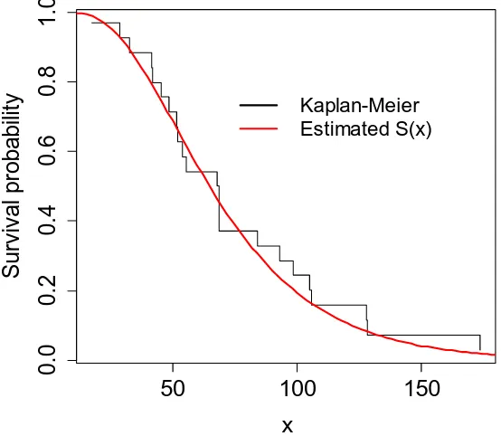
Figure 4: Estimated Survival function for the TNGIWD for ball bearings data

x

D

e

n

si

ty

0

50

100

150

0

.0

0

0

0

.0

0

5

0

.0

1

0

0

.0

1

5

TNGIW

NGIW

50 100 150

0

.0

0

.2

0

.4

0

.6

0

.8

1

.0

x

Su

rvi

va

l

p

ro

b

a

b

ili

ty Kaplan-Meier

Table 2 listed the MLEs of the unknown parameter(s) and the corresponding standard errors for the model parameters. In order to evaluate the performance of the TNGIW distribution and can be consider as a superior lifetime model, we shall compare the goodness of fit with five other lifetime distributions recently proposed in the literature. The visualization of the estimated densities with histogram displayed in Figure 3 indicate that the transmuted new generalized inverse Weibull distribution has the better estimates comparing with other five distributions. Hence the data points from the TNGIW distribution has better relationship and can be consider as the virtuous model for life time data. For the goodness of fit statistics, we use the Kolmogorov-Smirnov (K-S) test to see which model provides the better estimates and results are displayed in Table 2. In order to assess if the model is appropriate, Figure 4 plots the empirical and estimated survival functions of the TNGIW distribution.

Table 3: Cramér-von Mises, Anderson-Darling goodness of-fit statistics and K-S Test

Distribution 𝒲 𝒜 K-S Test

TNGIW 0.0318 0.1903 0.1061

KMIW 0.0338 0.1954 0.1115

EKIW 0.0346 0.2007 0.1149

NGIW 0.0335 0.1953 0.1105

KIW 0.0337 0.1955 0.1114

MIW 0.0752 0.5552 0.1328

To further verify which distribution provides the better estimates for ball bearings data, we apply the Cramér-von Mises and Anderson-Darling goodness of-fit statistics and results are displayed in Table 3. The smaller values of these statistics indicate the better fit. We detect from Tables 2 and 3 that the TNGIW distribution has the lowest values for the Kolmogorov-Smirnov (K-S) test, Cramér-von Mises and Anderson-Darling goodness of-fit statistics among the all fitted distributions recently proposed in the literature. Therefore the TNGIW distribution can be consider as a good model for the failure times of ball bearings data. Figures 4 displays the estimated Survival function of the TNGIW distribution with better relationship for the ball bearings data.

7.2. Application 2: Fatigue life of aluminium data

The second data set is prearranged by Birnbaum and Saunders (1969) on the fatigue life of 6061-T6 aluminium coupons cut parallel with the course of rolling and oscillated at 18 cycles per second. The data set comprises of 101 observations with maximum stress per cycle 31,000 psi. The data are

Table 4: MLEs of the Parameters for fatigue life of aluminium data and AIC

Model Parameter Estimates

𝛼̂ 𝛽̂ 𝛾̂ 𝜙̂ 𝜆̂

TNGIW 765.69 (933.96)

1.4084 (1.1478)

927.14 (1753.23)

313.48 (389.19)

0.8173 (0.1910)

KMIW 55.5137 143.61 1.4551 66.9352 5.5750

(199.86) (54.005) (0.7554) (173.34) (95.054) EKIW 33.6575 1.0858 1.6386 121.7002 21.0374 (65.1637) (0.9365) (1.6291) (328.69) (0.8763) NGIW 686.03

(693.55)

1.3005 (0.6479)

649.13 (1844.21)

362.14 (361.51)

-

KIW 71.1614 (306.61)

64.5064 (98.419)

90.4453 (389.55)

1.4842 (0.5042)

-

MIW 0.0001

(79.754)

3.0354 (0.0557)

2.24E+6 (1350.4)

- -

Figure 5: Fitted Models for failure of fatigue life aluminium data

x

D

e

n

si

ty

100

150

200

0

.0

0

0

0

.0

0

5

0

.0

1

0

0

.0

1

5

TNGIW

Table 5: Cramér-von Mises, Anderson-Darling goodness of-fit statistics and K-S Test

Distribution 𝒲 𝒜 K-S Test

TNGIW 0.0416 0.2893 0.0574

KMIW 0.0495 0.3507 0.0604

EKIW 0.0506 0.3376 0.0658

NGIW 0.0531 0.3830 0.0662

KIW 0.0496 0.3424 0.0639

MIW 0.2274 1.3069 0.2863

We examine the use of the use of the Transmuted new generalized inverse Weibull (TNGIW) distribution for modelling the fatigue fracture life of aluminium data. We fitted the TNGIW, NGIW, KMIW, EKIW, KIW and MIW densities are displayed in Table 4 and goodness of fit measures are listed in Table 5. The histogram of the fatigue fracture life of aluminium data is shown in Figure 5 along with the estimated densities of the TNGIW, NGIW models. The fitted model suggest that the TNGIW distribution is reasonable. These goodness of fit results indicate that the TNGIW distribution has the lowest values of the Kolmogorov-Smirnov (K-S) test, Cramér-von Mises and Anderson-Darling goodness of-fit statistics among the all fitted distributions. We conclude that the TNGIW distribution provides a good fit to these data sets.

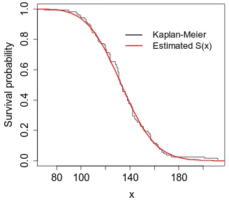
Figure 6: Estimated Survival function of TNGIWD for fatigue life aluminium data

80

100

140

180

0

.0

0

.2

0

.4

0

.6

0

.8

1

.0

x

Su

rvi

va

l

p

ro

b

a

b

ili

ty

8. Concluding Remarks

We studied and formulated some theoretical properties of the new distribution called the transmuted new generalized inverse Weibull distribution. The new distribution presents a generalization of several models previously considered in the literature such as transmuted modified inverse Weibull distribution, transmuted generalized inverse Weibull distribution, transmuted inverse Weibull distribution, modified inverse Weibull distribution. The proposed distribution has twenty three lifetime distributions as special cases. This proposed model has the upside down bathtub shape failure rate patterns. The method of maximum likelihood is employed for estimating the model parameters. The usefulness of the new model is illustrated in two applications. We have anticipation that the proposed model may attract wider applications in the analysis of lifetime data.

References

1. Aryal G. R., Tsokos C. P. (2011) Transmuted Weibull distribution: A Generalization of the Weibull Probability Distribution. European Journal of Pure and Applied Mathematics, Vol. 4: 2, 89-102.

2. Aryal G. R., Tsokos C. P. (2009). On the transmuted extreme value distribution with applications. Nonlinear Analysis: Theory, Methods and applications, Vol. 71, 1401-1407.

3. Aryal. G and Elbatal. I., (2015). Kumaraswamy Modified Inverse Weibull Distribution: Theory and Application, Appl. Math. Inf. Sci. 9, No. 2, 651-660. 4. Birnbaum, Z. W. and Saunders, S. C. (1969). Estimation for a family of life

distributions with applications to fatigue. Journal of Applied Probability, Vol. 6, pp. 328-347.

5. Elbatal, I. and Aryal, G. On the Transmuted Additive Weibull distribution, Aust. J. Stat, Vol. 42 (2), (2013a), 117–132.

6. Elbatal, I. Transmuted Modified Inverse Weibull distribution: A generalization of the modified Inverse Weibull probability distribution. International Journal of Mathematical Archive, Vol. 4 (8), (2013b), 117-129.

7. Gusmão, F.R.S., Ortega, E.M.M., Cordeiro, G.M., (2009). The generalized Inverse Weibull distribution. Statistical Papers. doi:10.1007/s00362-009-0271-3. 8. Khan M. Shuaib, Pasha, G.R and Pasha, A.H. Theoretical analysis of Inverse

Weibull distribution. WSEAS Transactions on Mathematics, 7(2), 2008, 30-38. 9. Khan M. Shuaib, King Robert, Modified Inverse Weibull Distribution, J. Stat.

Appl. Pro. 1, No. 2, (2012), 115-132.

10. Khan M. Shuaib, King Robert. (2013a). Transmuted Modified Weibull Distribution: A Generalization of the Modified Weibull Probability Distribution, European Journal of Pure and Applied Mathematics, Vol. 6: 1, 66-88.

12. Khan M. Shuaib, King Robert and Hudson Irene. (2014a). Characterizations of the transmuted Inverse Weibull distribution, ANZIAM J. Vol. 55 (EMAC2013), C197–C217.

13. Khan M. Shuaib and King Robert. (2014b). A New Class of Transmuted Inverse Weibull Distribution for Reliability Analysis, American Journal of Mathematical and Management Sciences, Vol. 33:4, 261-286.

14. Khan, M. Shuaib (2014). Modified Inverse Rayleigh Distribution, International Journal of Computer Applications, Vol. 87, No.13, 28-33.

15. Khan, M. Shuaib, King Robert., 2015. Transmuted Modified Inverse Rayleigh Distribution, Austrian Journal of Statistics, Vol. 44, No. 3, 2015, pp. 17-29. 16. Khan, M. Shuaib, King Robert. (2016). New generalized inverse Weibull

distribution for lifetime modeling, Communications for Statistical Applications and Methods, Vol. 23, No. 2, 147–161.

17. Klugman, S. A., Panjer, H. H. and Willmot, G. E. (2012), Loss Models, From Data to Decisions, Fourth Edition, Wiley.

18. Lawless, J.F. (1982), Statistic al Models and Methods for Lifetime Data, John Wiley and Sons, New York.

19. Merovci, F. (2013). Transmuted Rayleigh distribution. Austrian Journal of Statistics, Vol. 42, No. 1, 21-31.

20. Oguntunde, P.E. and Adejumo, A.O. (2015). The transmuted Inverse Exponential distribution. International Journal of Advanced Statistics and Probability, Vol. 3, No. 1, 1-7.

21. R Core Team (2013). R: A language and environment for statistical computing. R Foundation for Statistical Computing, Vienna, Austria. ISBN 3-900051-07-0, URLhttp://www.R-project.org/. R version 3.0.2.

22. Rodrigues. J. A., Silva. A. P. C. M., Hamedani. G.G., (2016). The exponentiated Kumaraswamy Inverse Weibull distribution, Journal of Statistical Theory and Applications, Vol. 15, No.1 (March 2016), 8-24.

23. Shahbaz, M.Q, Shahbaz, S, Butt N. S (2012). The Kumaraswamy Inverse Weibull distribution, Pak.j.stat.oper.res. Vol.VIII No.3, 479-489.

24. Vikas Kumar Sharma, Sanjay Kumar Singh, Umesh Singh, 2014. A new upside-down bathtub shaped hazard rate model for survival data analysis, Applied Mathematics and Computation, Vol. 239, 242–253.

25. Voda, V. Gh. (1972). On the Inverse Rayleigh Random Variable, Pep. Statist. App. Res., JUSE, 19, 13-21.

26. W. Shaw and I. Buckley. The alchemy of probability distributions: beyond Gram-Charlier expansions and a skew-kurtotic-normal distribution from a rank transmutation map. Research report, 2007.