Moment Properties And Quadratic Estimating Functions For Integer-Valued Time Series Models

for Integer-valued Time Series Models

Nurul Najihah Mohamad

Department of Computational and Theoretical Sciences,

Kulliyyah of Science, International Islamic University Malaysia 25200 Kuantan, Pahang, MALAYSIA

[email protected]

Ibrahim Mohamed

Institute of Mathematical Sciences, Faculty of Science, University of Malaya 50603, Kuala Lumpur, MALAYSIA

[email protected]

Ng Kok Haur

Institute of Mathematical Sciences, Faculty of Science, University of Malaya 50603, Kuala Lumpur, MALAYSIA

[email protected]

Abstract

Recently, there has been a growing interest in integer-valued time series models. In this paper, using a martingale difference, we prove a general theorem on the moment properties of a class of integer-valued time series models. This theorem not only contains results in the recent literature as special cases but also has the advantage of a simpler proof. In addition, we derive the closed form expressions for the kurtosis and skewness of the models. The results are very useful in understanding the behaviour of the processes involved and in estimating the parameters of the models using quadratic estimating functions (QEF). Specifically, we derive the optimal function for the integer-valued GARCH (p, q) known as INGARCH (p,

q) model. Simulation study is carried out to compare the performance of QEF estimates with corresponding maximum likelihood (ML) and least squares (LS) estimates for the INGARCH (1,1) model with different sets of parameters. Results show that the QEF estimates produce smaller standard errors than the ML and LS estimates for small sample size and are comparable to the ML estimates for larger sample size. For illustration, we fit the 108 monthly strike data to INGARCH (1, 1) models via QEF, ML and LS methods, and show the applicability of QEF method in practice.

Keyword: Skewness, kurtosis, martingale difference, quadratic estimating functions, integer-valued.

1. Introduction

An increasing number of studies that involve integer-valued time series data can be found in the literature. Zeger (1988) extensively studied the monthly cases of Polio infection in the U.S. from 1970 to 1983. Johansson (1996) considered the effect of lowering speed limits on the number of accidents while Li et al. (2014) investigated the implication of crime cases over time. As a result, there is a need for integer-valued time series models extended to include autoregressive moving average models, the first of which were introduced by Brockwell and Davis (1991) and Emad and Nadjib (1994).

introduced a new version of Ferland’s model with negative binomial deviate. For cases of data with excess zeroes, Zhu (2012) proposed the zero-inflated models with both Poisson and negative binomial deviates. Here, we re-examine some of these models and present simpler derivations of their moment properties using martingale difference. Such martingale difference have been successfully applied to various time series processes, see for example, Thavaneswaran and Abraham (1988) and Ghahramani and Thavaneswaran (2009). These results are very significant for the development of simpler theories on integer-valued time series models, in particular, for estimating the paramaters of the models using the estimating functions method.

The paper is divided as follows: In Section 2, we propose a general class of integer-valued time series models including important models given in Ferland et al. (2006), Zhu (2011) and Zhu (2012). We also derive the basic properties of the model, namely, formulae for the mean, variance, autocovariance and autocorrelation using a new approach, i.e by employing martingale differences. In Section 3, we present the higher order moment properties of the model up to order 4 by using martingale difference. In Section 4, we derive the optimal function for INGARCH (p,q) model via quadratic estimating functions (QEF). Simulation study is conducted to compare the performance of QEF, ML and LS estimates for INGARCH (1,1) model. We illustrate the QEF method in practice to the monthly strike data set given in Jung et al. (2005). Concluding remarks are given in Section 5.

2. Moments of Integer-Valued Time Series Models

Following the notation in Ferland et al. (2006), we consider four types of integer-valued time series model: Poisson (INGARCH), negative binomial (NBINGARCH), zero-inflated Poisson (ZIPINGARCH) and zero-zero-inflated negative binomial (ZINBINGARCH) with conditional mean E



X_t|_t1



is of the form:



Xt | t 1



a t,TP

E _   , (1)



 

 

 

 

q

j j t j p

i i t i

t X

1 ,TP 1

TP

,    

 , (2)

where _t1 is the  −field generated by X_t1,X_t2,...,X₁ with _t,TP is the intensity parameters with TP = Poisson (P), negative binomial (NB), zero-inflated Poisson (ZIP) and zero-inflated negative binomial (ZINB) for the respective models,  0, _i 0,

p

i 1,2,..., , and _j 0, j 1,2,...,q and a is the coefficient of the conditional mean with

     



  

) , , ( RCH for ZINBGA and

) , , ( ARCH for ZIPING 1

1 assuming

by ) , , ( NBINGARCH for

), , ( INGARCH for

1

t.NB

q p q

p

p p q

p r r

q p

a

t t

 



 ,

where r is the number of successful trials, p_t is the probability of successful trials and

We now apply the martingale difference, u_t  X_t E(X_t|_t1) X_t a_t,TP with 0

) (u_t 

E and Var(u_t)_u2. Multiplying equation (2) by a gives



 

 

 

 

q

j j t j p

i i t i

t a a X a

a

1 ,TP 1

TP

,    

 .

Since u_t is a martingale difference sequence, the equation can be rewritten in using backward operator, B, as

t q

j j j t

q

j j j p

i i

iB B X a B u

a _

  

 

      

 











 

1 1 1

1

1     . (3)

Now, let

 

     

q

j

j j p

i i

iB B

a B

1 1

1  

 and

 

  



q

j

j jB

B

1

1 

 . Then, equation (3) can

be represented in the form

 

B Xt a 

 

But

   . (4)

If all the roots of 

 

B 0 lie outside the unit circle, then the process

 

X_t is stationary. By letting

   

 

B B B

 

  and

 

B a 



  , the equation (4) can be written as

 

t

t B u

X  , i.e.

 

 

0 

j j t j

t u

X   , (5)

and the variance of X_t is given by



 

0 2 2 2

j j u t

X  

 .

Using first order stationarity, E(X_t) and since for large t, E(_t) approaches , a constant, then, _u2 can be easily expressed in terms of . For the processes INGARCH, NBINGARCH and ZIPINGARCH, it can be easily shown that the corresponding values

of _u2 are , 

     

r 

 1 and 

  

 

 

  

1

1 respectively. Moreover, for ZINBINGARCH

model, _u2 is given by





     

 

  

 

  

 

  

 

   

1 c for 1

1

0 c for 1

1 2

  



  



a a

u ,

et al. (2006). As highlighted by Zhu (2011, 2012), different approaches are required to exhibit the properties for the other three models and are of interest in future work.

The first aim here is to derive the general formula for the first two moments, the autocovariance and the autocorrelation of the integer-valued process

 

X_t of the form in equations (1-2). The result is given in Theorem 1.

Theorem 1: Under the first and second order stationarity assumptions,

(a)

 



 

  

 

q

j j p

i i t

a a X

E

1 1

1  



 ,

(b)

 

  

0 2 2 2

Var

j j u X t

X    ,

(c)  

0  2

j j j k u

X

k   

 ,

(d)

 

 _

 

 

0 2 0

j j j j j k X

k

  

 .

Proof: The mean of X_t can be obtained by taking the expectation of equation (3). Since 0

) (u_t 

E , 1(a) follows. From equation (5), we notice that the process can be represented as a general form of a time series process (see Abraham and Ledolter, 2009), therefore, the variance, autocovariance and correlation of X_t are obtained.

3. Skewness and Kurtosis

In the literature, only the first two moments and the autocovariance are given for integer-valued time series models. In this section, following Thavaneswaran et al. (2005), we obtained the general expression for the skewness and kurtosis for the INGARCH, NBINGARCH, ZIPINGARCH and ZINBINGARCH models.

Theorem 2: Consider a linear stationary process of the form    0 

j j t j

t u

X   where

 is the mean of the random process and u_t is an uncorrelated noise process with mean zero, variance _u2, skewness  u and kurtosis K u . Define S_t (X_t )2. Then, under suitable stationarity conditions, such process will have variance, skewness, kurtosis and correlation given by

(a)

 



 



 _

  

 

 



 



 

0

2

0 2 4

4 4

2 3

Var

j j u j j

u u

t K

(b)     2 / 3 0 2 0 3                j j j u j X   ,

(c)  

 





2 0 2 0 4 3 3                j j j j u X K K   , (d)  





 





 _          _                    0 2 0 2 4 0 2 0 2 2 2 3 2 3

j j j j

u

j j j k j j j k u S k K K        .

respectively. The proof is given in Appendix 1.

Example: Using Theorems 1 and 2, we derive the following results for four distributions with p = 1 and q = 1. From equations (1) and (2), the process

 

X_t is such that



Xt| t 1



a t,TP

E _   ,

TP , 1 1 1 1 TP

,   t  t

t   X  

 .

It can be shown that the weight _j is given by _j a₁(a₁₁)j1 where

          (1,1) GARCH for ZINBIN and (1,1) ARCH for ZIPING 1 1 assuming by (1,1) NBINGARCH for (1,1) INGARCH for 1 t.NB   t t p p r a .

Therefore, the summations of the weights _j are given in the following form:





2

1 1 2 1 1 1 0 2 1 2 1              _a a j j ,





3

1 1 3 1 2 1 1 1 2 1 2 0 3 1 3 3 1                 _a a a j j ,





4









               

  2

1 1 2 1 1 1 1 1 1 1 0 ₁ 1           a a a a k

j j j k

, and

















. 1 1 4 1 1 2 1 1 2 1 2 4 1 1 2 2 1 1 2 1 2 0 2 2                     _{ }           a a a a a a k

j j j k

From Theorem 1(c), the autocovariance of the

 

X_t process with order (1,1) can be written as













, 1 1 2 1 1 1 1 1 1 1 1 1 2                          a a a a k u X k

and from Theorem 1(b), the variance of the

 

X_t process is









, 1 1 2 1 1 2 1 2 2 1 1 2 2                      a a a u X

while from Theorem 1(d), the correlation of the

 

X_t process is

















 

, 1 1 2 1 2 1 1 1 1 1 1 1 1 1           a a a a a k X k        

where a is as defined earlier for the different models.

Using the same arguments as in Section 2, we can find the skewness and kurtosis of u_t.

The skewness  u for INGARCH, NBINGARCH and ZIPINGARCH is

 1 ,







    r r r 2

and







 









3/2

2 2 1 1 1 1 3 2 1                  

respectively. On the other hand,

the kurtosis, K u for INGARCH, NBINGARCH and ZIPINGARCH is respectively

 1 ,







      r r r r2 2 2 2

and K where K is











 



2

2 2 2 2 2 2 3 1 1 6 6 12 18 6 7 14 7 1                             .

4. General Theory of Quadratic Estimating Functions

Godambe (1960) was the first to introduce regular estimating functions (EF) that satisfy certain conditions and procedures for choosing an optimal EF. The requirement for a regular EF, g



X_t;θ



are:

(i) E



g



X_t;θ





g



X_t;θ

 

f X_t;θ



dX_t 0,

(ii)





θ θ  g X_t;

exists for all θ where is the parameter space,

(iii) _g



X_t;θ

 

f X_t;θ



dX_t is differentiable under the sign of integration,

(iv)



;



0

2    

  

θ θ

t

X g

E for all θ,

(v) Var



g



X_t;θ





E



g2



X_t;θ





.

According to Godambe (1960), to find the optimal EF, say g*



X_t;θ



two criteria should be satisfied. First, the estimated parameter should be as close as possible to the true

value. This means that the variance Var



g



X_t;θ





E



g2



X_t;θ





should be minimized and therefore E



g*2



X_t;θ





E



g2



X_t;θ





. The second criterion is that the expected values of the derivatives of the function g



X_t;θ



with respect to θ ,





   

 

  

  

θ θ

;

t

X g E

should be large as possible i.e.









   

 

  

        

  

    

  

 

θ θ θ

θ ;

; *

t

t _E g X

X g

E . By following both

criteria, the optimal EF, g*



X_t;θ



can be defined as follows:

Definition 1

Let G denote the class of all regular EFs. The g*



X_t;θ



G is said to be optimal if























;



.

;

; ;

2 2

2 *

2 *

   

 

  

   

    

  

    

  

 

θ θ

θ

θ θ

θ

t t

t t

X g E

X g E

X g E

X g E

Further, Godambe (1985) studied the inference of discrete time series processes using

estimating functions. He considered a class

 

   

 

 

 

n

t t t

h a g

g

1 1

: θ of EF which is linear

Theorem 3: Let

 

   

 

 

 

n

t t t

h a g

g

1 1

: θ be the class of all EFs where h_t and a_t1 are assumed to be differentiable with respect to θ for t 1,2,...,n. Then, the optimal

estimating function g*

 

θ minimizing













2

2

; ;

   

 

  

  

θ θ

θ

t t

X g E

X g E

is

 

   

n

t t t

h a g

1 *

1

* _{θ where}



1



2 1

*

1  

  

  

 

  

 t _{t t t}

t Eh

h E a

θ .

The EF method was later extended by Liang et al. (2011) to the case where the first four conditional moments are known. The functions used are called quadratic estimating functions (QEF).

Now, we assume that the discrete time stochastic process



X_t,t1,2,...,n



has the following conditional moments depending only on the parameter θ:

 

_



 _



 _{t t t1}

t  E X

 θ ,

 



 



_



 _{ }



 2 2 _1

2

t t

t t

t θ  E X  θ

 ,

 

 





 



1



3 3

1

  

  

 _{t t t}

t t

t E X θ

θ

θ 

 ,

 

 





 





3

1

1 4

4   



 _{t t t}

t t

t E X θ

θ

θ 

 

 .

We estimate the parameter θ using two classes of martingale differences

 



m_t θ m_t  X_t _t,t1,2,...,n



, (6)

and



s_t

 

θ s_t m_t2 _t2,t 1,2,...,n



, (7) such that

2 1 2

t t

t t E m

m  _ _{ } , (8)



2 ₁



 4



2



 _{t t t t}

t Es

s   , (9)



t t t



t t t Em s

s

m,  _1 3 . (10)

Theorem 4: In the class

 

 





             n

t t t t t Q

Q

Q g g a m b s

G

1 1 1

: θ

θ of all quadratic

estimating functions, the optimal estimating functions is given by

 

 







  

n

t t t t t

Q a m b s

g 1 * 1 * 1 * _θ where                           t t t t t t t t t t s m s m m s m s m

a 1 , 1 ,

2 1 2 * 1 θ θ   , and                          t t t t t t t t t t s s m s m s m s m

b 1 , , 1

2 1 2 * 1 θ θ   .

4.1 The INGARCH (p, q) Model

In this subsection, we focus on INGARCH (p, q) model given by



Xt | t 1



t,P

E _  ,

         q

j j t j p

i i t i

t X

1 ,P

1 P

,    

 .

The parameters of interest are θ



₀,₁,...,_p,₁,...,_q



'. The mean, variance, skewness and kurtosis of X_t conditional on _t1 are

P , P , P , 2 P , P , 1 and , 1 , ), ( t t t t t t t t

t     _  _

   θ     .

From equations (6) and (7), the martingale differences considered are m_t  X_t _t,P and





,P

2 P , t t t t X

s    . On the other hand, the conditional expectations in equations (8),

(9) and (10) are _t,P

t

m  , _t,P



1 2 _t,P



t

s    and , _t,P

t

s

m  . Let

P , P , 1 2 2 2 1 , 1 t t t t t t s m s m C               

. Then, from Theorem 4, the optimal QEF is

 

 







  

n

t t t t t

Q a m b s

and









. 0 2 1 1 2 1 1 2 2 1 1 , P , P , P , P , P , P , P , P , 2 * 1                                        t t t t t t t t t t t t t t t t s s m s m C b           θ θ

Therefore, one can conclude that, if the conditional mean and conditional variance are the same, the QEF method can be reduced to the EF method. Since we have pq1

parameters, then _t_,P(θ) are

                 j t i t t t _     

 ,P ,P ,P

P , (θ) , , , , , 1

1 1 1

P , , P , P ,                               q j q j q k j k t k P j t i j t j i t j t

j X _

        

where i1,2,...,p and j 1,2,...,q. Hence, the optimal QEF for each parameter are:

 



_,P



1

P , 1 ,P

* 1 1 t t q j j t j n t t Q X g       _               

 , (11)

 



,P



1

P , 1 ,P

* 1 t t q j i j t j i t n t t i

Q X X

g       _                

 , (12)

 



,P



1

P , P

, 1 ,P

* 1 t t q k j k t k j t n t t j Q X g        _                

 . (13)

The formulation of optimal equations for the other three models which are NBINGARCH (p,q), ZIPINGARCH (p,q) and ZINBINGARCH (p,q)models are the same as INGARCH (p,q) model. The optimal equation(s) for the additional extra parameter (s) in the above three models can be derived using optimal estimating functions in Theorem 4. An optimal estimate of θ can be obtained by solving the equation(s) g_Q*

 

θ 0.

4.2 Simulation Study

Let N and n be the number of simulations and the sample size generated respectively from the INGARCH (1, 1) models given by

Model 1: E



X_t|_t1



_t,P; _t,P 0.20.4X_t10.1_t1,P

Model 2: E



X_t|_t1



_t,P; _t,P 0.10.6X_t10.3_t1,P

Here, we demonstrate how to estimate the parameters using the QEF method:

• Step 1- Generate the data: We first generate the data from given true values. Then, we choose the observations numbering from 100 to 100 + n.

• Step 2- Initialize the parameters: We set the initial values for ₁ and ₁ by taking the typical values for each parameter, namely ₁0.1 and ₁0.8. On the other hand, we take the value of  to be the mean _X , of the generateddata in Step 1, namely,  0.1_X, (see Ferland et al., 2006).

• Step 3- Estimate the parameters: Using nleqslv, we solve the simultaneous optimal equations (11) to (13) in R-cran programming language in order to obtain the QEF estimates of  , ₁ and ₁ for the INGARCH (1,1) model.

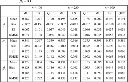
Table 1: Simulation results for INGARCH (1,1) with  0.2, 1 0.4 and

1 . 0 1 

 .

n = 100 n = 250 n = 500

ML LS QEF ML LS QEF ML LS QEF

Mean 0.167 0.241 0.170 0.198 0.185 0.185 0.202 0.190 0.191

ˆ Bias -0.032 -0.159 -0.030 -0.002 -0.015 -0.015 0.002 -0.010 -0.010

SE 0.067 0.101 0.057 0.049 0.048 0.046 0.035 0.037 0.034

RMSE 0.074 0.108 0.065 0.049 0.048 0.046 0.035 0.058 0.035

1

ˆ

 Mean 0.346 0.367 0.339 0.387 0.366 0.375 0.393 0.379 0.386

Bias -0.054 -0.033 -0.062 -0.012 -0.034 -0.025 -0.007 -0.021 -0.014

SE 0.126 0.145 0.129 0.089 0.098 0.089 0.060 0.062 0.060

RMSE 0.136 0.149 0.142 0.090 0.098 0.092 0.061 0.065 0.061

Mean 0.228 0.004 0.216 0.131 0.162 0.155 0.096 0.144 0.132

1

ˆ

 Bias 0.128 -0.096 0.116 0.013 0.062 0.055 -0.004 0.044 0.032

SE 0.185 0.265 0.145 0.131 0.116 0.111 0.092 0.092 0.086

RMSE 0.225 0.282 0.180 0.132 0.132 0.124 0.092 0.102 0.092

Discussion

Table 1: Simulation results for INGARCH (1,1) with  0.2, ₁ 0.4 and 1

. 0 1 

 (Cont.).

n = 1000 n = 1500

ML LS QEF ML LS QEF

Mean 0.201 0.196 0.197 0.201 0.197 0.198

ˆ Bias 0.001 -0.005 -0.003 0.001 -0.003 -0.002

SE 0.026 0.028 0.026 0.023 0.025 0.022

RMSE 0.027 0.028 0.027 0.023 0.025 0.022

1

ˆ

 Mean 0.399 0.395 0.396 0.399 0.396 0.399

Bias -0.001 -0.005 -0.004 -0.001 -0.004 -0.001

SE 0.041 0.045 0.042 0.031 0.037 0.030

RMSE 0.041 0.045 0.043 0.033 0.038 0.031

Mean 0.097 0.116 0.112 0.097 0.109 0.102

1

ˆ

 Bias -0.003 0.016 0.012 -0.003 0.009 0.002

SE 0.072 0.073 0.066 0.054 0.064 0.049

RMSE 0.072 0.075 0.067 0.055 0.064 0.050

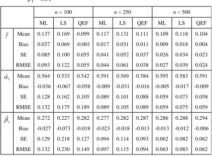
Table 2: Simulation results for INGARCH (1,1) with  0.1, ₁ 0.6 _and

3 . 0 1 

 .

n = 100 n = 250 n = 500

ML LS QEF ML LS QEF ML LS QEF

ˆ Mean 0.137 0.169 0.099 0.117 0.131 0.111 0.109 0.118 0.104 Bias 0.037 0.069 -0.001 0.017 0.031 0.011 0.009 0.018 0.004

SE 0.085 0.100 0.055 0.041 0.052 0.037 0.026 0.034 0.023

RMSE 0.093 0.122 0.055 0.044 0.061 0.038 0.027 0.039 0.024

1

ˆ

 Mean 0.564 0.533 0.542 0.591 0.569 0.584 0.595 0.583 0.591 Bias -0.036 -0.067 -0.058 -0.009 -0.031 -0.016 -0.005 -0.017 -0.009

SE 0.128 0.162 0.105 0.089 0.101 0.088 0.059 0.073 0.058

RMSE 0.132 0.175 0.189 0.089 0.105 0.089 0.059 0.075 0.059

1

ˆ

 Mean 0.272 0.227 0.282 0.277 0.282 0.287 0.286 0.288 0.294 Bias -0.027 -0.073 -0.018 -0.023 -0.018 -0.013 -0.013 -0.012 -0.006

SE 0.129 0.218 0.127 0.094 0.114 0.093 0.062 0.082 0.062

Table 2: Simulation results for INGARCH (1,1) with  0.1, ₁ 0.6and 3

. 0 1 

 (Cont.).

n = 1000 n = 1500

ML LS QEF ML LS QEF

ˆ _{Mean 0.104 0.111 0.102 0.103 0.108 0.102}

Bias 0.004 0.011 0.002 0.003 0.008 0.002

SE 0.016 0.024 0.016 0.013 -0.020 0.009

RMSE 0.017 0.026 0.017 0.014 0.022 0.011

1

ˆ

 _{Mean 0.598 0.594 0.596 0.595 0.597 0.598}

Bias -0.002 -0.01 -0.004 -0.005 -0.003 -0.002

SE 0.038 0.051 0.040 0.033 0.044 0.025

RMSE 0.038 0.051 0.040 0.033 0.044 0.026

1

ˆ

 _{Mean 0.294 0.289 0.297 0.294 0.291 0.297}

Bias -0.006 -0.01 -0.003 -0.005 -0.009 -0.003

SE 0.041 0.056 0.043 0.034 0.048 0.028

RMSE 0.042 0.057 0.043 0.034 0.049 0.030

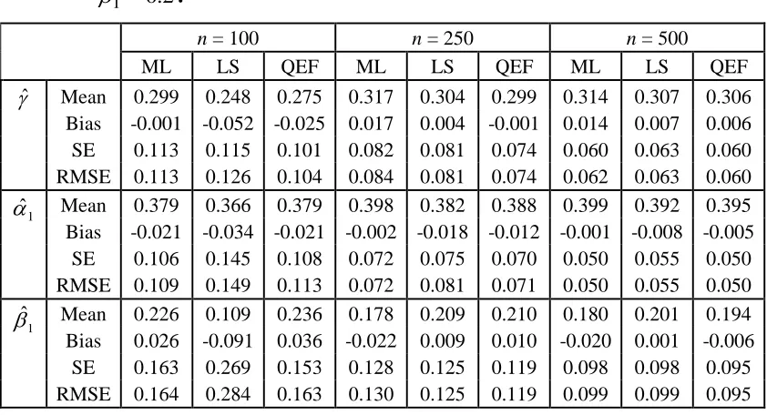
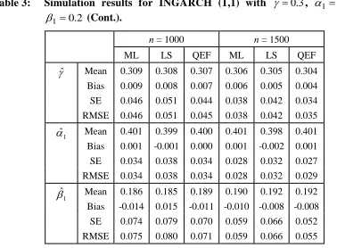
Table 3: Simulation results for INGARCH (1,1) with  0.3, 10.4 and

2 . 0 1 

 .

n = 100 n = 250 n = 500

ML LS QEF ML LS QEF ML LS QEF

ˆ Mean 0.299 0.248 0.275 0.317 0.304 0.299 0.314 0.307 0.306 Bias -0.001 -0.052 -0.025 0.017 0.004 -0.001 0.014 0.007 0.006 SE 0.113 0.115 0.101 0.082 0.081 0.074 0.060 0.063 0.060 RMSE 0.113 0.126 0.104 0.084 0.081 0.074 0.062 0.063 0.060

1

ˆ

 Mean 0.379 0.366 0.379 0.398 0.382 0.388 0.399 0.392 0.395 Bias -0.021 -0.034 -0.021 -0.002 -0.018 -0.012 -0.001 -0.008 -0.005

SE 0.106 0.145 0.108 0.072 0.075 0.070 0.050 0.055 0.050 RMSE 0.109 0.149 0.113 0.072 0.081 0.071 0.050 0.055 0.050

1

ˆ

 Mean 0.226 0.109 0.236 0.178 0.209 0.210 0.180 0.201 0.194 Bias 0.026 -0.091 0.036 -0.022 0.009 0.010 -0.020 0.001 -0.006

Table 3: Simulation results for INGARCH (1,1) with  0.3, ₁0.4 _and

2 . 0 1 

 (Cont.).

n = 1000 n = 1500

ML LS QEF ML LS QEF

ˆ Mean 0.309 0.308 0.307 0.306 0.305 0.304 Bias 0.009 0.008 0.007 0.006 0.005 0.004

SE 0.046 0.051 0.044 0.038 0.042 0.034

RMSE 0.046 0.051 0.045 0.038 0.042 0.035

1

ˆ

 Mean 0.401 0.399 0.400 0.401 0.398 0.401

Bias 0.001 -0.001 0.000 0.001 -0.002 0.001

SE 0.034 0.038 0.034 0.028 0.032 0.027

RMSE 0.034 0.038 0.034 0.028 0.032 0.029

1

ˆ

 Mean 0.186 0.185 0.189 0.190 0.192 0.192 Bias -0.014 0.015 -0.011 -0.010 -0.008 -0.008

SE 0.074 0.079 0.070 0.059 0.066 0.052

RMSE 0.075 0.080 0.071 0.059 0.066 0.055

A number of interesting results can be highlighted. Firstly, for the small sample sizes, ,

500 , 250 , 100



n the QEF estimates give the smaller values of SE and RMSE compared to other two methods. However, as n increases, the SE and RMSE values for the QEF estimates are always marginal smaller than ML and LS estimates. Secondly, as expected, as n increases from 100 to 1500, all the SE and RMSE of QEF, ML and LS estimates are consistently decreases. Lastly, it is important to point out the computational times for the QEF method is four times shorter than the ML method and three times shorter than the LS method when the simulation is done using R-cran programming. The R codes are available upon request.

Therefore, we can conclude that the QEF method provided consistently accurate estimates and computation effective than the ML and LS methods in the parameter estimation of INGARCH models.

4.3 Real data Example

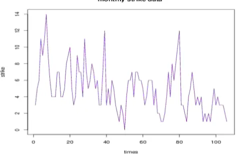
Figure 1: The monthly strike data from January 1994 to December 2002.

We fit the data using the INGARCH (1,1) model via the QEF, ML and LS methods. Then we obtain the parameter estimates together with their respective standard errors in parenthesis are shown in Table 4. We observe that, the QEF and ML methods give the same values of estimates. As expected, the standard errors of the QEF estimates are the smallest as compared to other two methods.

Table 4: The estimated parameters of INGARCH (1,1) model. Values in parentheses are standard errors of parameter estimates.

Method ˆ ˆ1 ˆ1

QEF 1.623 (0.428) 0.610 (0.081) 0.064 (0.114)

ML 1.623 (0.502) 0.610 (0.095) 0.064 (0.125)

LS 1.854 (0.512) 0.596 (0.112) 0.032 (0.128)

Then, to investigate the model fitting adequacy, we consider the Pearson residual defined

by

 

 

θˆ θˆ

P ,

P ,

t t t t

X z

 



 . According to Kedeem and Fakianos (2002), for the specified

model, the sequence z_t should have mean and variance close to0and1respectively and the sequence does not have serial correlation. We found that in our case, the mean and variance of the Pearson residuals are 0.032 and 1.009 respectively and are thus close to zero and unity as desired. Moreover, by using Ljung-Box (LB) statistics, the results from Table 5 indicate that there is no significant serial correlation in the residual.

Table 5: Diagnostics for INGARCH (1,1) model using QEF method.

LB(zt) LB( zt2)

χ2 28.1 21.3

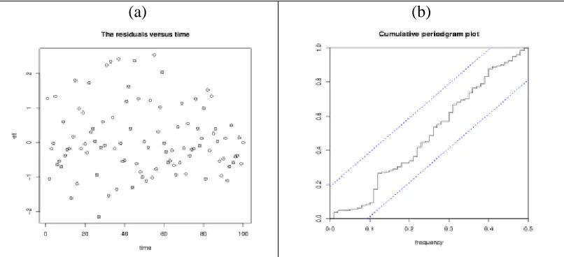
Furthermore, to examine the model adequacy, from Figure 2(a), there is no trend observed indicating the randomness of the residuals and in Figure 2(b), the plot does not exceed the dotted line. Therefore, the INGARCH (1, 1) model is a good fit for the monthly strike data given in Jung et al. (2005).

5. Concluding Remarks

This paper studied the moments of four integer-valued time series models, namely, the Poisson, negative binomial, zero-inflated Poisson and zero-inflated negative binomial models. We used the martingale difference to derive the higher order moments of all four models. The results for the first two moments are similar to those found in Zhu (2011) and Zhu (2012), but the derivation was much simpler. In addition, we derived the higher order moments of integer-valued time series up to order 4. However, the results hold for only the INGARCH (p, q) model. Further investigations on the stationarity of the other three models are required. Furthermore, we developed the quadratic estimating functions method mainly focusing on the INGARCH (p, q) model.

To investigate the performance of the QEF method compared to those of the LS and ML methods, simulation was carried out to obtain the estimated parameters together with their standard errors. The results showed that the QEF estimates give smaller standard errors and computation effective compared to the ML and LS estimates. Lastly, we model the monthly strike data using the INGARCH (1,1) model via QEF method. The adequacy of fit was investigated using diagnostic tools based on the Pearson residuals. For the future research, other estimation methods such as Kalman filter can be considered.

(a) (b)

Acknowledgement

This research is financially supported by Fundamental Research Grant Scheme No. FP012-2013A, University of Malaya Research Grant No. RP014C-15SUS and IIUM Research Initiative Grant Scheme No. RIGS16-311-0475.

References

1. Abraham, B., and Ledolter, J. (2009). Statistical Methods for Forecasting. John Wiley and Sons.

2. Aly, E.E.A.A., and Bouzar, N. (1994). On some integer-valued autoregressive moving average models. Journal of Multivariate Analysis,50(1), 132-151.

3. Brockwell, P.J., and Davis, R.A. (1991) Time Series: Theory and Methods, 2nd ed. Springer, New York.

4. Ferland, R., Latour, A., and Oraichi, D. (2006). Integer-valued GARCH process. Journal of Time Series Analysis, 27(6), 923-942.

5. Ghahramani, M. and Thavaneswaran, A. (2009). On some properties of autoregressive conditional Poisson (ACP) models. Economics Letters, 105(3), 273-275.

6. Godambe, V. P. (1960). An optimum property of regular maximum likelihood estimation. Annals of Mathematical Statistics, 31(4), 1208-1212.

7. Godambe, V. P. (1985). The foundations of finite sample estimation in stochastic processes. Biometrika, 72(2), 419-428.

8. Johansson, P. (1996). Speed limitation and motorway casualties: A time series count data regression approach. Accident Analysis & Prevention,28(1), 73-87. 9. Jung, R. C., Ronning, G., and Tremayne, A. R. (2005). Estimation in conditional

first order autoregression with discrete support. Statistical Papers,46(2), 195-224. 10. Kedeem, B., and Fokianos, K. (2002). Regression Models for Time Series

Analysis. John Wiley and Sons.

11. Li, G., Haining, R., Richardson, S., and Best, N. (2014). Space-time variability in burglary risk: A Bayesian spatio-temporal modelling approach. Spatial Statistics, 9, 180-191.

12. Liang, Y., Thavaneswaran, A., and Abraham, B. (2011). Joint estimation using quadratic estimating function. Journal of Probability and Statistics. (http://dx.doi.org/10.1155/2011/372512).

13. Thavaneswaran, A., and Abraham, B. (1988). Estimation for non-linear time series models using estimating equations. Journal of Time Series Analysis, 9(1), 99-108.

14. Thavaneswaran, A., Appadoo, S.S. and Peiris, S. (2005). Forecasting volatility. Statistics and Probability Letters, 75(1), 1-10.

15. Weiβ, C. H. (2010). The INARCH(1) model for overdispersed time series of counts. Communications in Statistics - Simulation and Computation, 39(6), 1269-1291.

17. Zhu, F. (2011). A negative binomial integer-valued GARCH model. Journal of Time Series Analysis, 32(1), 54-67.

18. Zhu, F. (2012). Zero-inflated Poisson and negative binomial integer-valued GARCH models. Journal of Statistical Planning and Inference,142(4), 826-839.

Appendix 1

(a) Let S_t 



X_t 



2. Then,

 









Var

 

,

0 2 2

2 _{  }

    j j u t t

t E X X

S

E   

and

 









 _{  }                               0 2 1 2 4 0 4 4 4 0 4 2 , 6 ,

i j i i j u

u j j u

j j t j t t K u E X E S E       

Since from the multinomial expansion, E

 

u_t 0 and E

 

u_t4 K u_u4. Similarly, we can show that                      0 4 2 0 2 0 2 1 2 . 3 3 6 j j j j i j i j

i  

 Hence,









 

 

 

 

     



3



2 .

3 3 6 Var Var 2 0 2 4 0 4 4 2 0 2 4 0 4 4 2 0 2 4 0 4 4 0 2 0 2 2 2 1 2 4 0 4 4 2 2 2                                 _                                     j j u j j u u j j u j j u j j u u j j u

i j i i j u j j u u j j u t t t t K K K S E S E S X                    

(b) Using the third moment and Theorem 1(b), the skewness of X_t is

 









 





3/2 3 Var _t t X X X

E 

    . 2 / 3 0 2 0 3 2 / 3 0 2 2 0 3 3                             j j j j u j j u u j j u      

(c) Using the fourth moment and Theorem 1(c), the kurtosis of X_t is

 

















 



 



. 3 3 3 3 2 0 2 0 4 2 0 2 4 0 4 4 2 0 2 4 0 4 4 2 2 4                                              j j j j u j j u j j u j j u j j u u t t X K K X E X E K            

(d) It is easily shown that





_{t i t j}

i j i i j j t j j

t

t X u u u

S  _{ }

              0 1 0 2 2 2

2  

 

and





2 .

0 1 0 2 2 2 j k t i k t i j i i j j t k j j

k t k

t X u u u

S  _{   }

                   

Since ut ’s are uncorrelated, we have





 





 



3



2 .

2 1 4 2 0 4 2 0 2 4 2 2 0 4 2 2 0 2 0 4 2 0 2 4 2 2 0 4 0 1 0 1 0 2 2 0 2 2                                                                                                      _                                             k j j j u j j u k j j j u u k j j j k j j j u j j u k j j j u u j k t i k t

i j i i j

j t i t

i j i i j

j t k j j

i t i i k t t K K u u u u E u u E S S E                        

Therefore, the covariance is given by







   



 





_                             2 0 4 2 2 0 4 ₂ 3 Cov k j j j u k j j j u u k t t k t t k t t K S E S E S S E S S       .

and the correlation is





 

 





 



3



2 .