www.clim-past.net/12/1645/2016/ doi:10.5194/cp-12-1645-2016
© Author(s) 2016. CC Attribution 3.0 License.
Mid-to-late Holocene temperature evolution and atmospheric
dynamics over Europe in regional model simulations
Emmanuele Russo and Ulrich Cubasch
Institute of Meteorology – FU-Berlin, Karl-Heinrich-Becker-Weg 6–10, 12165 Berlin, Germany
Correspondence to:Emmanuele Russo ([email protected])
Received: 19 January 2016 – Published in Clim. Past Discuss.: 2 February 2016 Revised: 4 July 2016 – Accepted: 29 July 2016 – Published: 17 August 2016
Abstract.The improvement in resolution of climate models
has always been mentioned as one of the most important fac-tors when investigating past climatic conditions, especially in order to evaluate and compare the results against proxy data. Despite this, only a few studies have tried to directly esti-mate the possible advantages of highly resolved simulations for the study of past climate change.
Motivated by such considerations, in this paper we present a set of high-resolution simulations for different time slices of the mid-to-late Holocene performed over Europe using the state-of-the-art regional climate model COSMO-CLM.
After proposing and testing a model configuration suit-able for paleoclimate applications, the aforementioned mid-to-late Holocene simulations are compared against a new pollen-based climate reconstruction data set, covering almost all of Europe, with two main objectives: testing the advan-tages of high-resolution simulations for paleoclimatic appli-cations, and investigating the response of temperature to vari-ations in the seasonal cycle of insolation during the mid-to-late Holocene. With the aim of giving physically plausible interpretations of the mismatches between model and structions, possible uncertainties of the pollen-based recon-structions are taken into consideration.
Focusing our analysis on near-surface temperature, we can demonstrate that concrete advantages arise in the use of highly resolved data for the comparison against proxy-reconstructions and the investigation of past climate change. Additionally, our results reinforce previous findings show-ing that summertime temperatures durshow-ing the mid-to-late Holocene were driven mainly by changes in insolation and that the model is too sensitive to such changes over Southern Europe, resulting in drier and warmer conditions. However, in winter, the model does not correctly reproduce the same
amplitude of changes evident in the reconstructions, even if it captures the main pattern of the pollen data set over most of the domain for the time periods under investigation. Through the analysis of variations in atmospheric circulation we sug-gest that, even though the wintertime discrepancies between the two data sets in some areas are most likely due to high pollen uncertainties, in general the model seems to underes-timate the changes in the amplitude of the North Atlantic Os-cillation, overestimating the contribution of secondary modes of variability.
1 Introduction
Climate has always a direct effect on all living organisms, and always will have an influence on human affairs (Wigley et al., 1981). From antiquity to the present day, human life and civilisation have been affected by the availability of natu-ral resources such as water, food, construction materials, etc. Under the current threat of global warming, understanding how climate will change in the next century has become of fundamental importance for the impact it could have on the life of our planet. Useful instruments for the study of climate change and its possible consequences are climate models. In general terms, a climate model can be defined as a mathe-matical representation of the climate system based on well-established physical principles (Randall et al., 2007).
the application of climate models for the study of changes in past climatic conditions.
An important case study is represented by the evolution of European climate during the mid-to-late Holocene (from 6000 years ago to present day). The large number of proxy data available and the particular configuration of the Earth astronomical parameters make it a useful period for the evaluation of the models’ response to changes in insolation (De Noblet et al., 1996; Kutzbach et al., 1996; Masson et al., 1999; Vettoretti et al., 2000; Bonfils et al., 2004; Bracon-not et al., 2007a, b; Mauri et al., 2014). During the mid-to-late Holocene, over northern latitudes in general, changes in the total amount of insolation during the year (with respect
to present-day conditions) were negligible (≤4.5 W m−2)
when compared to the seasonal variations (up to more than
30 W m−2for summer insolation at high latitudes) (Fischer
and Jungclaus, 2011). Indeed, relevant variations in the sea-sonal values of surface variables would be expected. How-ever, evidence shows that reconstructed climatic parameters, such as surface temperature, over Europe, did not always follow directly the astronomical forcings (Cheddadi et al., 1997; Davis et al., 2003; Bonfils et al., 2004; Braconnot et al., 2007a, b; Mauri et al., 2014), but their signal seems to have also been influenced by other complex processes such as atmospheric circulation, geography, or land-surface inter-actions with the atmosphere.
Different studies have been conducted in order to under-stand the mechanisms driving the seasonal behaviour of Eu-ropean surface variables during the mid-to-late Holocene. Cheddadi et al. (1997) showed that the results of a pollen-based reconstruction data set constrained by lake-level data, indicated that summer and winter temperatures were differ-ent over Northern and Southern Europe at the mid-Holocene in comparison to present-day values: winters, in particu-lar, were warmer over Northern Europe even if the insola-tion was reduced, while summers were colder over Southern Europe, despite the higher insolation. Similar results were obtained by Davis et al. (2003) who proposed an updated database of European pollen reconstructions for the entire Holocene. Bonfils et al. (2004), within the PMIP (Paleocli-mate Model Intercomparison Project, Joussaume and Taylor, 1995) collaboration, hypothesised that winter atmospheric patterns and summer soil conditions had an important influ-ence on seasonal changes of temperature and precipitation. This has also been highlighted by a study from Starz et al. (2013) who performed a simulation for the mid-Holocene with a coupled soil-ocean-atmosphere circulation model and dynamic vegetation, better reproducing soil water storage and heat fluxes. They found that changes in the soil’s phys-ical properties of the model led to improved model results and hampered anomalies in surface variables, with respect to proxy-data. Fischer and Jungclaus (2011) studied the evolu-tion of the European seasonal temperature cycle in a transient mid-to-late Holocene simulation with an ocean-atmosphere global climate model, although they were unable to
repro-duce correctly the reconstructed data over the entire region of study. In particular, their results presented only a weak shift to a positive phase of the NAO at mid-Holocene in win-ter, resulting in colder conditions over Northern Europe and warmer over Southern Europe, with respect to the values of reconstructions. In summer, again, the signal seemed to be mainly driven by changes in insolation, resulting in gener-ally warmer conditions over the entire domain and period of study. Conversely, in their recent work, Mauri et al. (2014) suggested that the different response of surface variables at the mid-Holocene was highly related to changes in atmo-spheric circulation both in winter and in summer. Specifi-cally, they proposed that in summer a major incidence of the “Scandinavian High” was most probably the reason for colder temperatures over Southern Europe 6000 years ago. In winter, on the contrary, a more positive phase of the North Atlantic Oscillation would have been responsible for warmer and wetter conditions over Northern Europe and an opposite behaviour in the South. Although these interpretations are all physically plausible, still general consensus is still missing on the correct explanation of the response of the climate sys-tem to changes in insolation for this period. Within the men-tioned studies, all the climate model applications have been conducted with transient simulations or considering a single time slice with global circulation models. In many cases the resolution of these simulations was not high enough to al-low for an assessment of the climate behaviour on a regional scale. As suggested by Renssen et al. (2001), if we want to evaluate the data against climatic reconstructions based on pollen data or any other record, an improvement in the reso-lution is required (Bonfils et al., 2004; Masson et al., 1999). Additionally, higher resolution is expected to lead to an im-provement of the results (Fischer and Jungclaus, 2011), al-lowing the representation of small-scale processes and more detailed information on surface and soil features (Feser et al., 2011).
Bearing this in mind, in recent years the application of re-gional climate models for paleoclimate studies has become more frequent. For example, Prömmel et al. (2013) used the COSMO-CLM in order to address the effect of changes in orography and insolation on African precipitation during the last interglacial. Fallah et al. (2016) investigated precipita-tions and dry periods during the Little Ice Age and the Me-dieval Warm Period over central Asia. Wagner et al. (2012) compared the mid-Holocene and pre-industrial climate over South America, while Felzer and Thompson (2001) evalu-ated a regional climate model for paleoclimate applications in the Arctic.
Figure 1.(Left) Anomalies of zonal mean insolation on top of the atmosphere (TOA) between 6000 years BP and pre-industrial period (PI). (Right) Mid-to-late Holocene trends of the anomalies, with respect to present-day values, of December and June TOA incoming insolation, calculated, according to Berger (1978), for 30 and 60◦North. Units are W m2.
for which changes in insolation due to astronomical forcings were negligible.
In this paper we employ for the first time a regional climate model, the COSMO-CLM (CCLM), for the investigation of the main climatic changes that characterized Europe during multiple time slices of the Mid-to-Late Holocene, with three main objectives:
– Propose and test a model configuration suitable for
pa-leoclimate studies
– Investigate the possible added value of highly resolved
simulations arising in the comparison against proxy-reconstructions
– Analyse proxy and model mismatches, providing
plau-sible physical interpretations of the dynamical pro-cesses responsible for them
Our discussion is structured as follows: in Sect. 2 the employed methodology, including a brief description of the models and the proxy data sets, is presented. Results are il-lustrated and discussed in Sect. 3: first a validation of the data for present-day conditions is conducted in order to test the performances of the model with the changes necessary for paleoclimate applications; then the mid-to-late Holocene simulations are compared against pollen-based reconstruc-tions, trying, in a first instance, to highlight the advantages of the performance of highly resolved simulations specifically for this case of study; finally, physically plausible interpre-tation of the mismatches between the CCLM results and the reconstructions are proposed; the results of other studies are additionally discussed.
2 Methods
2.1 Experimental Setup
In this work we perform a set of climate simulations, cov-ering several time slices of mid-to-late Holocene, employing models at different resolution.
The modus operandi consists of three parts and is based on
the so-calledtime slicetechnique (Cubasch et al., 1995):
1. First a transient continuous simulation is performed with the coupled atmosphere-ocean circulation model ECHO-G, composed by the ECHAM4 (Roeckner et al., 1996) and the ocean model HOPE (Wolff et al., 1997),
at a spectral resolution of T30 (∼3.75◦×3.75◦). Further
information on the simulation realisation are provided in Wagner et al. (2007).
2. We then select seven different time slices, at a temporal distance of approximately 1000 years from each other, from 6000 years ago down to the pre-industrial period, 200 years before present, in accordance to the time slices for which the pollen reconstructions are avail-able. For every time slice, a simulation is conducted, for a 30-year period, with the atmosphere-only global circulation model ECHAM5 (Roeckner et al., 2003) at
a spectral resolution of T106 (∼1.125◦×1.125◦), using
prescribed sea ice fraction and sea surface temperatures derived from the ECHO-G continuous run.
model by the German weather service (DWD) (Doms and Schättler, 2003).
In a first step we want to test whether the RCM setup and the applied model’s code modifications, required for imple-menting values of GHGs and astronomical forcings, are suit-able for paleoclimate studies. In order to set the values of astronomical parameters for the corresponding investigation periods, we apply the routine of Prömmel et al. (2013) that allows the estimation of latitudinal and seasonal insolation at the top of the atmosphere based on Earth’s astronomical parameters calculated by Berger (1978). In Fig. 1 the anoma-lies of zonal mean insolation on top of the atmosphere (TOA) between the pre-industrial period PI and 6000 years BP are presented. Additionally, the winter and summer mid-to-late
Holocene evolution of TOA insolation for 60 and 30◦North
are also shown in the same figure (Right). Additional changes to the original model code are required in order to set the
values of equivalent CO2concentration, representing
varia-tions in CH4, CO2and N2O. These data are deduced from air
trapped in ice cores (Flückiger et al., 2002). The contribution of the mid-to-late Holocene changes in GHGs concentration
to the radiative balance is negligible (less than 2 W m−2) in
comparison to the effects of changes in insolation, and only the latter are considered in our discussion.
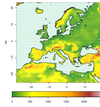
The setup of the COSMO-CLM is based upon the work of Hollweg et al. (2008) within the Euro-CORDEX Down-scaling experiment (Jacob et al., 2014). A more detailed de-scription of the model configuration used is provided in Ta-ble 1. For this study the model has been employed coupled to a soil–vegetation–atmosphere transfer scheme, the TERRA ML, a multi-layer model with a constant temperature lower boundary condition that allows one to reproduce the fluxes of heat, water and momentum between the soil surface and the atmosphere. Recent data of the physical parameters of the Earth’s surface (e.g., orography, land use, vegetation frac-tion, and land-sea mask) are employed for the simulations. The model domain, shown in Fig. 2, is the one used for the Euro-CORDEX simulations (Jacob et al., 2014), extending from Southern Greenland to Western Russia in the North and from the Western Atlantic coast of Morocco to the Red Sea in the South. Each simulation includes a 5-year spinup pe-riod used to let the model reach a semi-equilibrium state as suggested by Hollweg et al. (2008).
2.2 Observations
For the model validation for present climate, the E-OBS (Haylock et al., 2008) and the Climate Research Unit (CRU) (Harris et al., 2014) observational data sets are used as bench-marks for the comparison with the results of a COSMO-CLM control run covering the period 1991–2000 and driven by the ERAInterim (ERAInt) data set (Dee et al., 2011). The validation is conducted with respect to the total pre-cipitation and 2 m temperature winter and summer seasonal
−20 −10 0 10 20
−20
−10
0
10
20
rlon
rlat
0 500 1000 1500 2000 2500
m a.s.l.
Figure 2.Orography map of the COSMO-CLM simulation domain
in rotated coordinates.
Table 1.COSMO-CLM Main model configuration parameters.
Convection Tiedke
Time Integration Runge-Kutta,1T=240 s Robert-Aselin time filter
(alphaas)
0.53
Lateral Relaxation Layer 500 km
Radiation Ritter and Geleyn
Turbulence Implicit treatment of vertical diffusion using Neumann boundary conditions Rayleigh Damping Layer
(rdheight)
11 km
Soil Active Layers 9 Active Soil Depth 5.74 m
means. Additionally, CCLM heat fluxes and evapotranspira-tion values, from the same simulaevapotranspira-tion, are validated against the Global Land Data Assimilation System Version 1 Prod-ucts (GLDAS) dataset (Rodell et al., 2004).
2.3 Proxy reconstructions
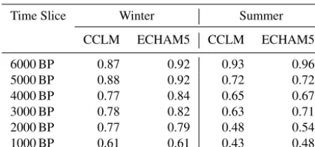
Table 2.Winter (left) and summer (right) temperature cost function estimates for the CCLM and the ECHAM5 models compared to the Proxy reconstructions for each time slice of mid-to-late Holocene. Values closer to 0 indicate a better agreement with proxy recon-structions.
Time Slice Winter Summer
CCLM ECHAM5 CCLM ECHAM5
6000 BP 0.87 0.92 0.93 0.96
5000 BP 0.88 0.92 0.72 0.72
4000 BP 0.77 0.84 0.65 0.67
3000 BP 0.78 0.82 0.63 0.71
2000 BP 0.77 0.79 0.48 0.54
1000 BP 0.61 0.61 0.43 0.48
corrected with postglacial isostatic readjustment. Along with the data, a standard error estimate derived from the transform and the interpolation methods is also provided. Reconstruc-tions contain information on seasonal (winter and summer) and annual values of precipitation and temperature, as well as a measure of moisture balance and of growing degree days
over 5◦, and are provided on a regular grid with a resolution
of 1×1 longitude degrees.
The choice of the data set of Mauri et al. (2015) has been done for several reasons. First of all, it allows us to per-form a comparison against the model results over most of the simulation domain, considering different variables (even if we only focus on temperature in our discussion). Then, it covers exactly the same time slices of our model simu-lations: no other data set has this temporal and spatial cov-erage at such high spatial resolution. Additionally, the ro-bustness of the data has been thoroughly tested, in Mauri et al. (2015), against other proxies (including chironomids,
δ18O from speleothems and lake ostracods, bog-oaks,
glacio-lacustrine sediments, wood anatomy and other pollen recon-structions based on different reconstruction methods) lead-ing to satisfactory results. Nonetheless, similar pollen-based climatic reconstructions have been extensively employed in other data-model comparisons, and, most recently, for the evaluation of the PMIP3/CMIP5 climate models included in the last IPCC report (Stocker et al., 2013; Harrison et al., 2015).
3 Results and discussion
3.1 Model validation and evaluation for present day
As a first step a control simulation has been performed with present values of orbital parameters and greenhouse gases (Sect. 2) in order to test the ability of the CCLM, modified accordingly to our purposes, to properly reproduce present-day climate. Additionally, this provides further knowledge about the spatial distribution of the model performances.
The simulation covers a 10-year period, between 1991 and 2000. Even if the length of this simulation can be considered as “critical” for the model’s validation, we want to acknowl-edge that, due to computational reasons, it was not possible to cover a longer period.
In Figs. 3 and 4, winter and summer seasonal means of temperature (left panel) and precipitation (right panel) from the CCLM simulations are compared against the CRU and the E-Obs observational data sets.
In the first column of each panel, the climatology of the different data sets is shown: the model is able to correctly re-produce, within a certain degree of accuracy, the climatology of the observations for both temperature and precipitation in winter and in summer.
In the right column of every panel, temperature and precip-itation values from the present-day control run are directly
validated, through a Student’s t test, against the CRU and
the E-Obs data sets. The same test is conducted for evap-oration and heat fluxes but against the GLDAS data set in Fig. 5. In these figures the black dots represent the grid cells
where the null hypothesis of the t test, assuming that the
data being sampled could be drawn from the same under-lying distribution, is not rejected at a significance level of 5 %. The biases between the CCLM results and the observa-tions are represented with different colours. The results show that, for temperature, the model performs well over North-ern Europe in both winter and summer. Winter-time results are in particularly good agreement with observations over Northeastern Europe and Scandinavia (Fig. 3, column II).
However, larger deviations (up to 4◦C in some cases) are
present over Central Europe, Turkey and Northern Africa. In particular the model tends to simulate generally colder conditions over these regions. Winter precipitation results seem to be in good agreement over a major part of the do-main, with some deviations from the observations over re-gions with particularly complex orography, in rere-gions that are normally highly affected by westerlies and in the North-ern African coasts of the Mediterranean Sea (where the bi-ases are particularly pronounced, and the model results di-verge by almost 100 % from the values of the observations) (Fig. 3, column IV). In summer, instead, the main discrep-ancies are found over Southern Europe both for tempera-ture and precipitation (Fig. 4). In particular the temperatempera-ture
anomalies exceed 3◦C over most of the Mediterranean
Figure 3.Analysis ofWinterseasonal means of 2 m temperature (left panel) and Precipitation (right panel) for the period 1991–2000. The first column of each column (I, III) shows the mean climatology for the investigated period as represented in the three considered data sets: the CCLM in the first row, the CRU in the second and the E-OBS at the bottom. The second columns show (II, IV), instead, the biases between the CCLM results and the respective observational data sets. The area with a point represent the grid cells where the anomalies between the two data sets are not significant, according to a Student’sttest, at a significance level of 5 %.
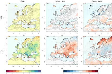
of energy transferred by the latent heat flux. This increases the sensible heat flux, ultimately leading to an increase of air temperature, on the one-hand, and to a decrease of local precipitation on the other (Zveryeav and Allan, 2010).
Based on these considerations, we suggest that the model reproduces anomalously warm and dry conditions over a wide part of Southern Europe and the Mediterranean basin, during summer, as a consequence of a wrong conversion of energy towards latent heat in these regions. This hypothesis is supported by the heat fluxes and evapotranspiration maps (Fig. 5) presenting a spatial distribution of the anomalies re-sembling the ones of temperatures and precipitation. In par-ticular, the model underestimates latent heat flux and evap-otranspiration, while overestimating sensible heat over the corresponding area.
Nevertheless the performances of the model with the ap-plied changes are in good agreement with the results of
other works focusing on the same region (Hollweg et al., 2008; Kotlarski et al., 2014; Schimanke et al., 2012; Gómez-Navarro et al., 2011, 2013), having in general the same fea-tures and spread of the anomalies. Indeed the applied changes and configuration appear to be exploitable for paleoclimate applications.
3.2 Possible added value of highly resolved simulations for paleoclimate studies
Figure 4.As Fig. 3 but forSummer.
in the interpretation of proxy data that are often influenced by processes taking place on smaller scales than the ones resolved in coarser models, they are supposed to be a par-ticularly suitable tool for paleoclimate studies. Within this context, in our discussion we try to highlight the importance of using high resolution models, and in particular regional climate models, for the simulation of past climate change.
Aiming at investigating the value added by highly resolved simulations for the comparison of changes in near-surface temperatures against proxy-reconstructions, we follow a two-step approach:
1. Firstly, we conduct a qualitative analysis of the simula-tions performed with three models at different resolu-tion in order to detect visible differences in the repro-duced signals.
2. Secondly, we employ a quantitative approach in or-der to estimate the skills of the RCM, in comparison to the driving GCM, in reproducing the same mid-to-late Holocene changes in temperature as derived from proxy-reconstructions.
As a benchmark for such comparison we use the pollen-based temperature reconstructions of Mauri et al. (2015). In this way, we aim at establishing whether the representation of smaller scale processes and improved orographic features of the region of study could lead to results that are in better agreement with the mentioned proxy-based reconstructions.
Figure 5.Biases of seasonal means of Evapotranspiration (left), Latent (centre) and Sensible Heat (right) fluxes, between the CCLM sim-ulations and the GLDAS data set, calculated for the reference period 1991–2000. As in the previous figures, the area with a point represent the grid cells where the anomalies between the two data sets are not significant, according to a Student’sttest, at a significance level of 5 %.
Winterresults are presented in the first row, andSummerresults in the second.
Italy and Scandinavia are partly or completely masked-out in this case.
Consequently, we focus further analysis on the comparison between the ECHAM5 and the CCLM results. In both sea-sons additional details are easily detectable in the CCLM pat-tern. The coastline is also better reproduced in this case, re-sulting in a better detailed representation of the land-sea con-trast, a more precise reproduction of surface processes and, consequently, leading to more suitable information for possi-ble comparison against proxy-data. Nonetheless, the CCLM shows better defined patterns as a consequence of higher res-olution, being able to discriminate higher spatial variability.
On the basis of such analysis, in the successive step, we try to quantify how better the CCLM reproduces the recon-structed temperatures in comparison to the ECHAM5. For this purpose we use an approach similar to the one employed by Zhang et al. (2010) and based on the work of Goosse et al. (2006). After regridding by bilinear interpolation the CCLM and the ECHAM5 results on the reconstructions grid, we in-troduce a cost function defined as
CFkmod=
v u u t
1
n
n X
i=1
ωik(Treck ,i−T k
mod,i)
2, (1)
where CFkmodis the value of the cost function for each
con-sidered time slice of mid-to-late Holocenekand each model.
The parameter n represents the number of the
reconstruc-tions’ grid boxes.Treck ,i is the temperature of the proxy-data
at every locationi, whileTmodk ,i is the corresponding
temper-ature of the model simulation. Additionally, the parameter
wki takes into account the uncertainties of the reconstructions
at every location and time period. Its value is given by
ωik= 1
(SEki)2+1, (2)
where SEi represents the standard error of the
reconstruc-tions at every grid box i. The corresponding uncertainties
of the model results are considerably small (∼0.01◦C) in
comparison to the ones of the reconstructions, similarly to Goosse et al. (2006), and are indeed neglected. In this way reconstructions with higher uncertainties will contribute less in the calculation of the cost function.
The values of the cost function for the two models are pro-vided in Table 2. Values closer to 0 indicate a better agree-ment with proxy reconstructions.
T 2M anomalies 6000 BP-PI
DJF JJA
P
O
LLE
N
C
C
LM
E
C
HAM
5
E
C
HO
G
−10 0 10 20 30 40 50
30
40
50
60
70
lon
lat
−10 0 10 20 30 40 50
30
40
50
60
70
lon
lat
−20 −10 0 10 20
−20
−10
0
10
20
rlon
rlat
−20 −10 0 10 20
−20
−10
0
10
20
rlon
rlat
−10 0 10 20 30 40 50
30
40
50
60
70
lon
lat
−10 0 10 20 30 40 50
30
40
50
60
70
lon
lat
−10 0 10 20 30 40 50
30
40
50
60
70
lon
lat
−10 0 10 20 30 40 50
30
40
50
60
70
lon
lat
−6 −4 −2 0 2 4 6
oC
Figure 6.Maps of the anomalies between 6000 BP and the
prein-dustrial period ofWinter(left) andSummer(right) seasonal means of 2 m temperature, calculated over a 25-year period. The results of the three different models and the pollen-based reconstructions are presented. From top to bottom: POLLEN-based reconstructions, CCLM, ECHAM5, ECHO-G. The results are presented on each data set original grid: the CCLM data, in particular, are shown in rotated geographical coordinates.
In particular the CCLM results are, in some cases, closer by more than 10 % to the reconstructions. It is important to mention that the scale of the pollen-based reconstructions, considered for our analysis, is closer to the resolution of the
ECHAM5 than of the CCLM. As suggested by Di Luca et al. (2015), given that the main difference between the GCM and the RCM is related to their horizontal resolution, it seems natural that the results depend on the spatial scale of the anal-ysis. Additionally, it is key to state that the evinced results are relative to this case study and other comparisons should be performed, considering different couples of RCM-GCM, in order to derive more robust conclusions on the suitability of higher-resolution models for the comparison against proxy-reconstructions. Nonetheless, the motivation behind produc-ing higher resolution climate simulations is not only related to scientific arguments of the type described above. From a different perspective, such results, due to the greater level of detail, could be preferable for applications in studies in which human adaptation or environmental response to past climatic changes would be investigated. Accordingly, the need for cli-mate information at very fine scales, for applications such as archaeology or vegetation reconstructions, constitutes a strong incentive to perform higher-resolution climate sim-ulations (Di Luca et al., 2015; Rummukainen, 2016). The evinced results and the proposed discussion give us concrete motivation for the choice of conducting RCM simulations for this particular case study.
3.3 The CCLM results and their anomalies in the comparison with reconstructions
Finally we focus on the comparison between the CCLM re-sults and the pollen-based reconstructions. After analysing the differences between the two data sets and their temporal evolution, we propose, by means of correlations with trends of insolation and changes in atmospherical circulation pat-terns, physically plausible interpretation of the evinced mis-matches.
Figures 7 and 8 present the temperature biases between the two data sets for winter and summer seasonal means, re-spectively. These are calculated, after upscaling the CCLM results on the grid of the pollen-based reconstructions by bilinear interpolation, for every time slice of mid-to-late Holocene. Additionally, they are accompanied by the maps of the corresponding pollen uncertainties.
In winter, generally colder conditions are reproduced by the model over northern continental Europe, with slightly warm biases over most of the South (Fig. 7). In Scandinavia a negative bias is present for the first two millennia, after which the situation then reverses. The largest anomalies (in
some cases up to∼4◦C) are present over Northeastern
Eu-rope (likely related to high pollen-data uncertainty partly due to the fact that seasonal values derived from pollen in this area are biased towards the winter season) and Turkey.
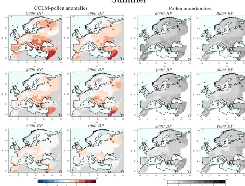
In summer, instead, CCLM results present positive anoma-lies over most of the domain, with particularly pronounced
values (in some case larger than∼4◦C) over different parts
Winter
CCLM-pollen anomalies6000 BP 5000 BP
✲✁ ✁ ✁ ✷ ✁ ✸ ✁ ✹ ✁ ✺ ✁ ✂ ✄ ☎ ✄ ✆ ✄ ✻ ✄ ✼ ✄ ❧✝✞ ✟✠ ✡ ✲✁ ✁ ✁ ✷✁ ✸✁ ✹✁ ✺✁ ✂ ✄ ☎ ✄ ✆ ✄ ✻ ✄ ✼ ✄ ❧✝✞ ✟✠ ✡
4000 BP 3000 BP
✲✁ ✁ ✁ ✷ ✁ ✸ ✁ ✹ ✁ ✺ ✁ ✂ ✄ ☎ ✄ ✆ ✄ ✻ ✄ ✼ ✄ ❧✝✞ ✟✠ ✡ ✲✁ ✁ ✁ ✷✁ ✸✁ ✹✁ ✺✁ ✂ ✄ ☎ ✄ ✆ ✄ ✻ ✄ ✼ ✄ ❧✝✞ ✟✠ ✡
2000 BP 1000 BP
✲✁ ✁ ✁ ✷ ✁ ✸ ✁ ✹ ✁ ✺ ✁ ✂ ✄ ☎ ✄ ✆ ✄ ✻ ✄ ✼ ✄ ❧✝✞ ✟✠ ✡ ✲✁ ✁ ✁ ✷✁ ✸✁ ✹✁ ✺✁ ✂ ✄ ☎ ✄ ✆ ✄ ✻ ✄ ✼ ✄ ❧✝✞ ✟✠ ✡ ✲✹ ✲✷ ✁ ✷ ✹ oC Pollen uncertainties
6000 BP 5000 BP
☛☞✌ ✌ ☞✌ ✍✌ ✎✌ ✏✌ ✑✌ ✒ ✓ ✔ ✓ ✕ ✓ ✖ ✓ ✗ ✓ ✘✙✚ ✛✜ ✢ ☛☞✌ ✌ ☞✌ ✍✌ ✎✌ ✏✌ ✑✌ ✒ ✓ ✔ ✓ ✕ ✓ ✖ ✓ ✗ ✓ ✘✙✚ ✛✜ ✢
4000 BP 3000 BP
☛☞✌ ✌ ☞✌ ✍✌ ✎✌ ✏✌ ✑✌ ✒ ✓ ✔ ✓ ✕ ✓ ✖ ✓ ✗ ✓ ✘✙✚ ✛✜ ✢ ☛☞✌ ✌ ☞✌ ✍✌ ✎✌ ✏✌ ✑✌ ✒ ✓ ✔ ✓ ✕ ✓ ✖ ✓ ✗ ✓ ✘✙✚ ✛✜ ✢
2000 BP 1000 BP
☛☞✌ ✌ ☞✌ ✍✌ ✎✌ ✏✌ ✑✌ ✒ ✓ ✔ ✓ ✕ ✓ ✖ ✓ ✗ ✓ ✘✙✚ ✛✜ ✢ ☛☞✌ ✌ ☞✌ ✍✌ ✎✌ ✏✌ ✑✌ ✒ ✓ ✔ ✓ ✕ ✓ ✖ ✓ ✗ ✓ ✘✙✚ ✛✜ ✢ ✌ ☞ ✍ ✎ ✏ ✑ oC
Figure 7.Left: maps ofWinter2 m temperature anomalies between CCLM and pollen-based reconstructions for the different time slices
of mid-to-late Holocene. Right: standard error of winter temperature seasonal mean derived from the pollen-based reconstructions for each time slice of mid-to-late Holocene.
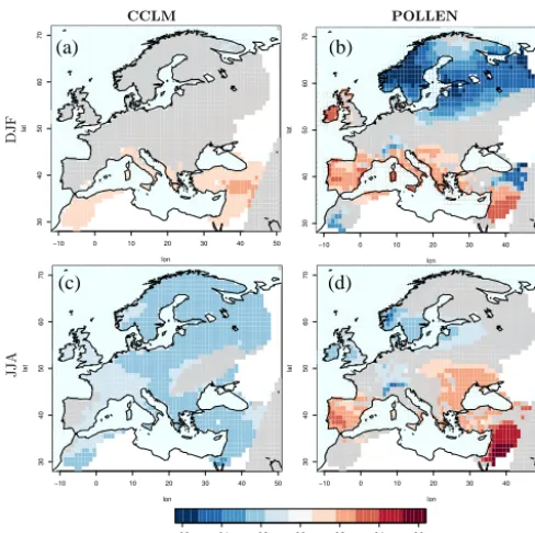
In addition to the previous analyses, the maps of temper-ature temporal evolution are presented in Fig. 9. They show the slope of the mid-to-late Holocene linear trends of tem-perature anomalies with respect to the pre-industrial period, calculated at every grid box by means of a weighted least squares method, taking into account the contribution of the different uncertainties. The points for which the trends are not significant, according to an F-test at a significance level of 10 %, are masked out in grey.
From these maps we see that in winter, even if over part of Southern Europe the two data sets present similar trends, their behaviour is different in the North: CCLM results show no significant trend (Fig. 9a), while the pollen-based recon-structions present significantly decreasing temperatures over a considerable part of the domain (Fig. 9b). In particular, over Scandinavia, while the pollen-based reconstructions show a strong, significant cooling trend, no significant trend is evi-dent for the model results. Conversely, in summer, the model
Summer
CCLM-pollen anomalies6000 BP 5000 BP
✲✁ ✁ ✁ ✷ ✁ ✸ ✁ ✹ ✁ ✺ ✁ ✂ ✄ ☎ ✄ ✆ ✄ ✻ ✄ ✼ ✄ ❧✝✞ ✟✠ ✡ ✲✁ ✁ ✁ ✷✁ ✸✁ ✹✁ ✺✁ ✂ ✄ ☎ ✄ ✆ ✄ ✻ ✄ ✼ ✄ ❧✝✞ ✟✠ ✡
4000 BP 3000 BP
✲✁ ✁ ✁ ✷ ✁ ✸ ✁ ✹ ✁ ✺ ✁ ✂ ✄ ☎ ✄ ✆ ✄ ✻ ✄ ✼ ✄ ❧✝✞ ✟✠ ✡ ✲✁ ✁ ✁ ✷✁ ✸✁ ✹✁ ✺✁ ✂ ✄ ☎ ✄ ✆ ✄ ✻ ✄ ✼ ✄ ❧✝✞ ✟✠ ✡
2000 BP 1000 BP
✲✁ ✁ ✁ ✷ ✁ ✸ ✁ ✹ ✁ ✺ ✁ ✂ ✄ ☎ ✄ ✆ ✄ ✻ ✄ ✼ ✄ ❧✝✞ ✟✠ ✡ ✲✁ ✁ ✁ ✷✁ ✸✁ ✹✁ ✺✁ ✂ ✄ ☎ ✄ ✆ ✄ ✻ ✄ ✼ ✄ ❧✝✞ ✟✠ ✡ ✲✹ ✲✷ ✁ ✷ ✹ oC Pollen uncertainties
6000 BP 5000 BP
☛☞✌ ✌ ☞✌ ✍✌ ✎✌ ✏✌ ✑✌ ✒ ✓ ✔ ✓ ✕ ✓ ✖ ✓ ✗ ✓ ✘✙✚ ✛✜ ✢ ☛☞✌ ✌ ☞✌ ✍✌ ✎✌ ✏✌ ✑✌ ✒ ✓ ✔ ✓ ✕ ✓ ✖ ✓ ✗ ✓ ✘✙✚ ✛✜ ✢
4000 BP 3000 BP
☛☞✌ ✌ ☞✌ ✍✌ ✎✌ ✏✌ ✑✌ ✒ ✓ ✔ ✓ ✕ ✓ ✖ ✓ ✗ ✓ ✘✙✚ ✛✜ ✢ ☛☞✌ ✌ ☞✌ ✍✌ ✎✌ ✏✌ ✑✌ ✒ ✓ ✔ ✓ ✕ ✓ ✖ ✓ ✗ ✓ ✘✙✚ ✛✜ ✢
2000 BP 1000 BP
☛☞✌ ✌ ☞✌ ✍✌ ✎✌ ✏✌ ✑✌ ✒ ✓ ✔ ✓ ✕ ✓ ✖ ✓ ✗ ✓ ✘✙✚ ✛✜ ✢ ☛☞✌ ✌ ☞✌ ✍✌ ✎✌ ✏✌ ✑✌ ✒ ✓ ✔ ✓ ✕ ✓ ✖ ✓ ✗ ✓ ✘✙✚ ✛✜ ✢ ✌ ☞ ✍ ✎ ✏ ✑ oC
Figure 8.As in Fig. 7 but forSummerseasonal means.
Storch and Zwiers, 1995). In CCA, according to Gómez-Navarro et al. (2015), “from a physical point of view, the leading patterns should show similar characteristics when the mechanisms leading to the relationships between the climate fields are controlled by the same processes”.
In our analysis we adopt the method of Barnett and Preisendorfer (1987) in which an EOF analysis is conducted prior to the CCA, retaining only a few leading EOFs, in or-der to remove part of the random noise from the data. More specifically, after conducting the EOF analysis on the anoma-lies, with respect to the pre-industrial period, of MSLP and T2M, we select the first eight principal components of both the variables in winter, and the first eight and twelve princi-pal components of, respectively, MSLP and T2M in summer. In this way, in both the cases, the selected PCs will explain approximately 80 % of the total variance in the original data sets. We then apply the CCA analysis on the retrieved PCs.
Figures 10 and 11 show the first two canonical pairs of patterns with the largest canonical correlation for both winter and summer.
CCLM POLLEN
D
JF
JJ
A
−10 0 10 20 30 40 50
30 40 50 60 70 lon lat
−10 0 10 20 30 40 50
30 40 50 60 70 lon lat
−10 0 10 20 30 40 50
30 40 50 60 70 lon lat
−10 0 10 20 30 40 50
30 40 50 60 70 lon lat
−0.6 −0.4 −0.2 0.0 0.2 0.4 0.6
oC kyr
(a) (b)
(c) (d)
–1
Figure 9.Mid-to-late Holocene temporal Evolution of the
anoma-lies, with respect to the pre-industrial period, of near-surface tem-perature winter (first row) and summer (second row) seasonal means, derived from the CCLM simulations (left) and the pollen-based reconstruction (right). The maps show the slopes of the linear trends calculated, for every grid box, taking into consideration the uncertainties associated to the two data sets, by means of a weighted least squares method. The area masked out in grey, are the area where the trends are not significant, according to a F-test at a sig-nificance level of 10 %.
In summer, instead, the first CCA pair (Fig. 11a, b) seems to be highly related to changes in insolation (Fig. 13a, b). It is key to note that, the first canonical pattern of summer MSLP anomalies and its structure, seems to be a proper product of this particular case of study. Even if it implies changes in circulation, we do not see any particularly prominent dipole structure characteristic of other well-known circulation pat-terns for the region. Its effects on temperature are particularly high on the Atlantic coast of continental Europe, resulting in a smoothing of the trend of summer temperature over this region.
In the second CCA pair, the pattern of the mean sea level pressure (Fig. 11c) resembles the positive phase of the Summer North Atlantic Oscillation (SNAO) (Folland et al., 2009). The trend (Fig. 13c) of its expansion coefficients is again not particularly pronounced. As a consequence, the changes in the corresponding temperature pattern (Fig. 13d) are also not remarkable.
Consequently, we suggest that in summer, during mid-to-late Holocene, the changes in circulation alone would not have been enough to explain the variations in surface temper-ature, as reconstructed from the proxies. While over
North-MSLP T2M
−80 −60 −40 −20 0 20
30 40 50 60 70 rlon rlat −0.9 −0.8 −0.7 −0.6 −0.5 −0.4 −0.3 −0.2 −0.1 −0.1 0 0 0 0 0.1 0.1 0.2 0.2 0.2 0.3 0.3 0.3 0.4
−20 −10 0 10 20
−20 −10 0 10 20 rlon rlat −0.3 −0.2 −0.2 −0.1 −0.1 −0.1 0 0 0 0 0 0 0.1 0.1
0.1 0.1
0.1 0.1 0.1 0.1 0.2 0.2
0.2 0.2
0.2 0.2 0.2 0.2 0.2 0.3 0.3 0.3 0.3 0.3 0.3 0.3 0.3 0.4 0.4 0.4 0.4 0.4 0.4 0.4 0.5 0.5 0.5 0.6 0.6 0.6 0.6 0.7 0.7 0.8
−1.0 −0.5 0.0 0.5 1.0 −80 −60 −40 −20 0 20
30 40 50 60 70 rlon rlat −0.7 −0.6 −0.5 −0.4 −0.3 −0.2 −0.1 0 0 0.1 0.1 0.1 0.2 0.2 0.3 0.3 0.3 0.4 0.4 0.5
0.5 0.5
0.6
0.6
0.6
0.7
0.8
−20 −10 0 10 20
−20 −10 0 10 20 rlon rlat −0.8 −0.7 −0.7 −0.7 −0.6 −0.6 −0.6 −0.6 −0.5 −0.5 −0.5 −0.5
−0.4 −0.3
−0.3 −0.3 −0.2 −0.2 −0.2 −0.1 −0.1 −0.1 −0.1 0 0 0 0 0 0 0 0 0.1 0.1 0.1 0.1 0.2 0.2 0.2 0.2 0.2 0.3
0.3 0.3
0.3 0.3 0.3 0.4 0.4 0.4 0.5 0.5 0.5 0.5 0.6 0.6 0.6 0.7 0.7 0.7 R=0.91 R=0.89
12.32 % 22.02 %
33.63 % 19.62 %
(a)
(b)
(c)
(d)
Figure 10.Canonical correlation pattern pairs of MSLP (left) and
T2M (right) inWinter, calculated accordingly to the Barnett and Preisendorfer (1987) method. Each panel illustrates the percentage of variance explained by the patterns and the canonical correlation associated with the pair. The results are calculated for the mid-to-late Holocene, from 6000 BP to pre-industrial times. Note that the MSLP has been obtained directly from the driving GCM, since the window of interest lies outside the RCM domain. For both the vari-ables the analysis has been conducted on the standardised anoma-lies with respect to the pre-industrial period. Red (blue) areas in-dicate positive (negative) correlations, for each grid point, between the data and the corresponding canonical score series.
ern Europe the relatively good agreement between the tem-perature of the two data sets over part of the domain sug-gests that for this region the insolation is probably the main driver of change; for Southern Europe, however, the role of land-atmosphere coupling needs to be considered (Senevi-ratne et al., 2006).
MSLP T2M
−80 −60 −40 −20 0 20
30 40 50 60 70 rlon
rlat −0.8
−0.7 −0.6 −0.5 −0.4 −0.3 −0.3 −0.3 −0.2 −0.2 −0.2 −0.2 −0.1 −0.1 −0.1 −0.1 0 0 0 0 0.1 0.1 0.1 0.2 0.3 0.4 0.4
−20 −10 0 10 20
−20 −10 0 10 20 rlon rlat −0.7 −0.7 −0.6 −0.6 −0.6 −0.5 −0.5 −0.4 −0.4 −0.4 −0.3 −0.3 −0.3 −0.2 −0.2 −0.2 −0.2 −0.1 −0.1
−0.1 −0.1
−0.1 −0.1 0 0 0 0 0 0 0 0 0 0 0.1 0.1 0.1 0.1 0.1 0.1 0.1 0.2 0.2 0.2 0.2 0.2 0.2 0.3 0.3 0.3 0.3 0.4 0.4 0.4 0.4 0.4 0.5 0.5 0.5 0.5 0.5 0.5
0.6 0.6
0.6
0.6
0.6
0.7 0.7
0.7 0.7
−1.0 −0.5 0.0 0.5 1.0
−80 −60 −40 −20 0 20
30 40 50 60 70 rlon rlat −0.6 −0.6 −0.5 −0.5 −0.4 −0.4 −0.3 −0.3 −0.2 −0.2 −0.1 −0.1 0 0 0 0 0.1 0.1 0.1 0.2 0.2 0.2 0.3 0.3 0.4 0.5 0.6 0.7 0.8
−20 −10 0 10 20
−20 −10 0 10 20 rlon rlat −0.4 −0.3 −0.3 −0.3 −0.3 −0.3 −0.3 −0.2 −0.2 −0.2 −0.2 −0.2 −0.1 −0.1 −0.1 −0.1 −0.1 −0.1 0 0 0 0 0 0 0 0 0 0.1 0.1 0.1 0.1 0.1 0.1 0.1 0.1 0.1 0.2 0.2 0.2 0.2 0.2 0.2 0.2 0.2 0.2 0.3 0.3 0.3 0.3 0.3 0.3
0.3 0.4 0.4 0.4 0.4 0.4 0.5 0.5 0.5 0.5 0.5 0.6 0.6 0.7 0.7 0.8 0.8 R=0.87 R=0.81
7.07 % 16.77 %
20.24 % 14.91 %
(a)
(b)
(c)
(d)
Figure 11.As in Fig. 10 but forSummerseason.
consequently, to drier and warmer conditions. Further experi-ments, with improved soil properties, are indeed necessary in order to better reproduce soil moisture content, and to obtain more robust results for the comparison with reconstructions. It is important to mention that the behaviour of mid-to-late Holocene’s summer temperature over Europe has been highly debated during recent years. While a dipole behaviour between Southern and Northern Europe has been suggested by several studies based on pollen analyses (Huntley and Prentice, 1988; Cheddadi et al., 1997; Prentice et al., 1998; Davis et al., 2003; Mauri et al., 2015) and others relying on a combination of different proxies, such as the one of Magny et al. (2013), which suggested a North-South paleoclimatic contrast in the central Mediterranean during the Holocene, other studies argued against such a hypothesis. In particular Osborne et al. (2000) proposed that reconstructions of sum-mer temperature based on pollen could be erroneous for the Mediterranean region, since here the vegetation distribution is mainly limited by effective precipitation, rather than by summer temperature.
The latest hypothesis should be taken into account for the comparison between pollen-based reconstructions and model simulations. Nevertheless, additional investigations have shown that, when directly compared to the pollen record, the mid-Holocene vegetation simulated from the out-put of climate models is way too dry over Southern Eu-rope, with an expansion of Mediterranean and steppe/desert vegetation and contraction in forest cover, a direct conse-quence of simulated warmer conditions (Prentice et al., 1998; Wohlfahrt et al., 2004; Gallimore et al., 2005; Benito Garzon et al., 2007; Kleinen et al., 2010).
Based on these considerations, recognizing the data set of Mauri et al. (2015) as a valuable source for the investiga-tion of European temperature evoluinvestiga-tion during mid-to-late Holocene, we acknowledge the fact that joint efforts from specialists of different disciplines are still required in order to further clarify possible uncertainties.
3.3.1 Other modelling studies
An important benchmark for the comparison of our results against other modelling studies is represented by the out-comes of the PMIP3 experiment (Braconnot et al., 2011), for which several simulations have been performed, with dif-ferent coupled circulation models, for the mid-Holocene and the pre-industrial time. Here we focus on the results of 12 of the PMIP3 simulations. Specifically, we perform a di-rect comparison of the regional mean of winter and summer near-surface temperature calculated for Northern and South-ern Europe for the PMIP3 simulations as well as each of ours. The results are presented in two tables, provided as Supplement, in which the corresponding values derived from the pollen-based reconstructions are also included. Two main features arise from such analysis: first of all common positive
anomalies (∼ +1◦C) over Southern Europe in summer for
all the models is evident, while the reconstructions present
a negative value (∼ −1.2◦C). This indicates that the
tem-perature differences are positive in the model simulations as a result of the higher summer insolation at mid-Holocene than at the pre-industrial period. Additionally, another fea-ture that seems to be common to all the models is repre-sented by the failure in representing winter anomalies in both the regions and it is attributable to a wrong reproduction of changes in the amplitude of NAO (Fischer and Jungclaus, 2011; Strandberg et al., 2014). While some models present a value similar to the one of reconstructions for Southern
Eu-rope (∼ +0.5◦C), in the North the differences are
signifi-cant, with the pollen-based reconstructions presenting warm
anomalies (∼ +2.5◦C), and the models having slightly
pos-itive values (between 0 and+1◦C) in some cases, and
nega-tive (up to∼ −1◦C) in the others.
4 Summary and conclusions
In this work we performed for the first time a set of highly resolved climate simulations over Europe for different time-slices of mid-to-late Holocene, by means of the state-of-the-art regional climate model COSMO-CLM.
As a first step, using the CRU and the E-OBS observa-tional data sets as benchmarks, a model setup suitable for paleoclimate investigations has been tested for the reference period 1991–2000. The results show that the RCM is able to reproduce realistic climatology with respect to the obser-vations. The largest biases arise in summer over Southern Europe where the model reproduces warmer and drier
precipita-MSLP T2M
−3
−2
−1
0
1
2
3
Years BP
6000 5000 4000 3000 2000 1000 200
−3
−2
−1
0
1
2
3
Years BP
6000 5000 4000 3000 2000 1000 200
−3
−2
−1
0
1
2
3
Years BP
6000 5000 4000 3000 2000 1000 200
−3
−2
−1
0
1
2
3
Years BP
6000 5000 4000 3000 2000 1000 200
(a)
(b)
(c)
(d)
Figure 12. Canonical score series of the first two pairs of canonical correlation patterns of, respectively, MSLP (left column) and 2 m
temperature (right column) winter seasonal mean anomalies.
tion), likely related to a wrong conversion of energy towards latent heat over this area. Nevertheless, the results are in good agreement with the ones of other studies for the same region, and the employed configuration can be considered a valid reference for future applications.
Successively, the results of mid-to-late Holocene simula-tions have been compared against a new pollen-based cli-mate reconstruction data set. Winter and summer seasonal means of near-surface temperature have been considered for our analysis.
To begin with, the possible advantages of higher resolu-tion models for paleoclimate applicaresolu-tions have been investi-gated. The RCM seems to better reproduce the signal of the climate-reconstruction when compared to the driving GCMs, with a more detailed reproduction of the coast-line and bet-ter defined patbet-terns. Additionally, using a quantitative ap-proach, we have demonstrated that the results of the RCM are closer to the values of the reconstructions in comparison to the driving GCM, in some cases by more than 10 %. Con-sidering also the final user perspective, the evinced results gave us concrete reasons for choosing to conduct highly re-solved simulations for this particular case study.
Finally, the CCLM results are used in order to investigate the response of the climate system to changes in the seasonal cycle of insolation, with the aim of proposing plausible phys-ical interpretations of the mismatches arising in the compar-ison against the reconstructions.
MSLP T2M
−3
−2
−1
0
1
2
3
Years BP
6000 5000 4000 3000 2000 1000 200
−3
−2
−1
0
1
2
3
Years BP
6000 5000 4000 3000 2000 1000 200
−3
−2
−1
0
1
2
3
Years BP
6000 5000 4000 3000 2000 1000 200
−3
−2
−1
0
1
2
3
Years BP
6000 5000 4000 3000 2000 1000 200
(a)
(b)
(c)
(d)
Figure 13.As in Fig. 12 but for summer.
times, again mainly due to insolation changes, the pollen data exhibit an opposite trend. According to the results of previ-ous works and to the analysis of atmospheric dynamics, we suggest that this behaviour is mainly due to a higher parti-tion of radiaparti-tion towards latent heat, resulting in a cooling effect of the surface that the model is not able to reproduce due to deficiencies in the representation of soil-atmosphere heat fluxes over this area. Nonetheless, it is important to men-tion that the validity of reconstrucmen-tions of European summer temperature over the Mediterranean region based on pollen data has been highly questioned in recent years. Even though several evidences confirm an increasing trend of temperature over the area from 6000 BP to present day, joint efforts from specialists of different disciplines are still required in order to further clarify possible uncertainties.
This paper sets the basis for further investigations: in par-ticular a set of new simulations with improved radiation schemes, soil properties and land use, could lead to impor-tant contributions to climate modelling and, consequently, to the improvement of future climate change projections.
5 Data availability
Pollen-based reconstructions used in this study were pub-lished in Mauri et al. (2015) and are available at: http:// arve.unil.ch/pub/EPOCH-2_Mauri_etal_QSR.tar.gz. For the access to the climate simulations results, please directly con-tact the authors.
The Supplement related to this article is available online at doi:10.5194/cp-12-1645-2016-supplement.
Acknowledgements. The authors are grateful to the two
for designing and conducting the ECHAM5 climate simulations. A particular acknowledgment goes to Edoardo Mazza for his continuous support and intellectual debate. We would also like to thank Ingo Kirchner, Bijan Fallah, Nico Becker, Alexander Walter and John Walter Acevedo Valencia for the fruitful and interesting discussions. Additionally, we are particularly grateful to Jacque-line Harvey for proofreading the manuscript.
Edited by: H. Goosse
Reviewed by: two anonymous referees
References
Barnett, T. and Preisendorfer, R.: Origins and levels of monthly and seasonal forecast skill for United States surface air tem-peratures determined by canonical correlation analysis, Mon. Weather Rev., 115, 1825–1850, 1987.
Benito Garzon, M., Sánchez de Dios, R., and Sáinz Ollero, H.: Predictive modelling of tree species distributions on the Iberian Peninsula during the Last Glacial Maximum and Mid-Holocene, Ecography, 30, 120–134, 2007.
Berger, A.: Long-term variations of daily insolation and Quaternary climatic changes, J. Atmos. Sci., 35, 2362–2367, 1978. Bonfils, C., de Noblet, N., Guiot, J., and Bartlein, P.: Some
Mecha-nisms of mid-Holocene climate change in Europe, inferred from comparing PMIP models to data, Clim. Dynam., 23, 79–98, 2004.
Braconnot, P., Otto-Bliesner, B., Harrison, S., Joussaume, S., Pe-terchmitt, J.-Y., Abe-Ouchi, A., Crucifix, M., Driesschaert, E., Fichefet, Th., Hewitt, C. D., Kageyama, M., Kitoh, A., Laîné, A., Loutre, M.-F., Marti, O., Merkel, U., Ramstein, G., Valdes, P., Weber, S. L., Yu, Y., and Zhao, Y.: Results of PMIP2 coupled simulations of the Mid-Holocene and Last Glacial Maximum – Part 1: experiments and large-scale features, Clim. Past, 3, 261– 277, doi:10.5194/cp-3-261-2007, 2007a.
Braconnot, P., Otto-Bliesner, B., Harrison, S., Joussaume, S., Pe-terchmitt, J.-Y., Abe-Ouchi, A., Crucifix, M., Driesschaert, E., Fichefet, Th., Hewitt, C. D., Kageyama, M., Kitoh, A., Loutre, M.-F., Marti, O., Merkel, U., Ramstein, G., Valdes, P., Weber, L., Yu, Y., and Zhao, Y.: Results of PMIP2 coupled simula-tions of the Mid-Holocene and Last Glacial Maximum – Part 2: feedbacks with emphasis on the location of the ITCZ and mid- and high latitudes heat budget, Clim. Past, 3, 279–296, doi:10.5194/cp-3-279-2007, 2007b.
Braconnot, P., Harrison, S., Otto-Bliesner, B., Abe-Ouchi, A., Jung-claus, J., and Peterschmitt, J.: The Paleoclimate Modeling Inter-comparison Project contribution to CMIP5, Clivar Echanges No. 56, 16, No. 2, 15–19, 2011.
Cheddadi, R., Guiot, J., Harrison, S., and Prentice, I.: The climate of Europe 6000 years ago, Clim. Dynam., 13, 1–9, 1997. Christensen, J., H., Boberg, F., Christensen, O., and Picher, P.: On
the need for bias correction of regional climate change projec-tions of temperature and precipitation, Geophys. Res. Lett., 35, L20709, doi:10.1029/2008GL035694, 2008.
Collins, M. and Allen, M.: On assessing the relative Roles of ini-tial and boundary Conditions in interannual to decadal Climate Predictability, J. Climate, 15, 3104–3109, 2002.
Cubasch, U., Waszkewitz, J., Hegerl, G., and Perlwitz, J.: Regional climate changes as simulated in time-slice experiments, Climatic Change, 31, 273–304, 1995.
Davis, B., Brewer, S., Stevenson, A., and Guiot, J.: The temperature of Europe during the Holocene reconstructed from pollen data, Quaternary Sci. Rev., 22, 1701–1716, 2003.
De Noblet, N., Braconnot, P., Joussaume, S., and Texier, D.: Sensi-tivity of simulated Asian and African summer monsoons to or-bital induced variations in insolation 126, 115 and 6 kBP, Clim. Dynam., 15, 162–603, 1996.
Dee, D., Uppala, S., Simmons, A., Berrisford, P., Poli, P., Kobayashi, S., Andrae, U., Balmaseda, M., Balsamo, G., Bauer, P., Bechtold, P., Beljaars, A., van de Berg, L., Bidlot, J., Bor-mann, N., Delsol, C., Dragani, R., Fuentes, M., Geer, A., Haim-berger, L., Healy, S., Hersbach, H., Holm, E., Isaksen, L., Kall-berg, P., Köhler, M., Matricardi, M., McNally, A., Monge-Sanz, B., Morcrette, J., Park, B., Peubey, C., de Rosnay, P., Tavolato, C., Thépaut, J., and Vitart, F.: The ERA-Interim reanalysis: con-figuration and performance of the data assimilation system, Q. J. Roy. Meteor. Soc., 137, 553–597, 2011.
Di Luca, A., de Elia, R., and Laprise, R.: Challenges in the Quest for Added Value of Regional Climate Dynamical Downscaling, Curr. Clim. Change Rep., 1, 10–21, 2015.
Doms, G. and Schättler, U.: A Description of the nonhydrostatic re-gional model LM, Part II: Physical Parameterization, Tech. rep., Consortium for Small Scale Modelling (COSMO), 2003. Fallah, B., Sahar S., and Ulrich C.: Westerly jet stream and past
millennium climate change in Arid Central Asia simulated by COSMO-CLM model, Theor. Appl. Climatol. 124, 1079–1088, 2016.
Felzer, B. and Thompson, S.: Evaluation of a Regional Climate Model for paleoclimate applications in the Arctic, J. Geophys. Res., 106, 407–427, 2001.
Feser, F., Rocker, B., von Storch, H., Winterfeldt, J., and Zahn, M.: Regional Climate Models add Value to Global Model Data: a Re-view and Selected Examples, B. Am. Meteorol. Soc., 92, 1181– 1192, 2011.
Fischer, E., Seneviratne, S., Vidale, P., Lüthi, D., and Schär, C.: Soil moisture-atmosphere interactions during the 2003 European summer heat wave, J. Climate, 20, 5081–5099, 2007.
Fischer, N. and Jungclaus, J. H.: Evolution of the seasonal tempera-ture cycle in a transient Holocene simulation: orbital forcing and sea-ice, Clim. Past, 7, 1139–1148, doi:10.5194/cp-7-1139-2011, 2011.
Flückiger, J., Monnin, E., Stauffer, B., Schwander, J., Stocker, T., Chappellaz, J., Raynaud, D., and Barnola, J.: High resolution Holocene N2O ice core record and its relationship with CH4and CO2, Global Biogeochem. Cy., 16, doi:10.1029/2001GB001417, 2002.
Folland, C., Knight, J., Linderholm, H., Fereday, D., Ineson, S., and Hurrell, J.: The Summer North Atlantic Oscillation: Past, Present, and Future, J. Climate, 22, 1082–1103, 2009.
Gallimore, R., Jacob, R., and Kutzbach, J.: Coupled atmosphere-ocean-vegetation simulations for modern and mid-Holocene cli-mates: role of extratropical vegetation cover feedbacks, Clim. Dynam., 25, 755–776, 2005.
millennium, Clim. Past, 7, 451–472, doi:10.5194/cp-7-451-2011, 2011.
Gómez-Navarro, J. J., Montávez, J. P., Jiménez-Guerrero, P., Jerez, S., Lorente-Plazas, R., González-Rouco, J. F., and Zorita, E.: Internal and external variability in regional simulations of the Iberian Peninsula climate over the last millennium, Clim. Past, 8, 25–36, doi:10.5194/cp-8-25-2012, 2012.
Gómez-Navarro, J. J., Montávez, J. P., Wagner, S., and Zorita, E.: A regional climate palaeosimulation for Europe in the period 1500–1990 – Part 1: Model validation, Clim. Past, 9, 1667–1682, doi:10.5194/cp-9-1667-2013, 2013.
Gómez-Navarro, J. J., Bothe, O., Wagner, S., Zorita, E., Werner, J. P., Luterbacher, J., Raible, C. C., and Montávez, J. P.: A regional climate palaeosimulation for Europe in the period 1500–1990 – Part 2: Shortcomings and strengths of models and reconstruc-tions, Clim. Past, 11, 1077–1095, doi:10.5194/cp-11-1077-2015, 2015.
Goosse, H., Renssen, H., Timmermann, A., Bradley, R., and Mann, M.: Using Paleoclimate proxy-data to select optimal realisations in an ensemble of simulations of the climate of the past millen-nium, Clim. Dynam., 27, 165–184, 2006.
Hagemann, S., Machenhauer, B., Jones, R., Christensen, O., Déqué, M., Jacob, D., and Vidale, P.: Evaluation of water and energy budgets in regional climate models applied over Europe, Clim. Dynam., 23, 547–567, 2004.
Harris, I., Jones, P., Osborn, T., and Lister, D.: Updated high-resolution grids of monthly climatic observations- the CRU TS3.10 dataset, Int. J. Climatol., 34, 623–642, 2014.
Harrison, S., Bartlein, P., Izumi, K., Li, G., Annan, J., Hargreaves, J., Braconnot, P., and Kageyama, M.: Evaluation of CMIP5 palaeo-simulations to improve climate projections, Nat. Clim. Change, 5, 735–743, 2015.
Haylock, M., Hofstra, N., Klein Tank, A., Klok, E., Jones, P., and New, M.: European daily high-resolution gridded dataset of sur-face temperature and precipitation for 1950–2006, J. Atmos. Sci., 112, D20119, doi:10.1029/2008JD010201, 2008.
Hollweg, H., Böhm, U., Fast, I., Hennemuth, B., Keuler, K., Keup-Thiel, E., Lautenschlager, M., Legutke, S., Radtke, K., Rockel, B., Schubert, M., Will, A., Woldt, M., and Wunram, C.: Ensem-ble Simulations over Europe with the Regional Climate Model CLM forced with IPCC AR4 Global Scenarios, Tech. rep., Max Planck Institute für Meteorologie, 2008.
Huntley, B. and Prentice, C.: July temperatures in Europe from pollen data, Science, 241, 687–690, 1988.
Jacob, D., Kotlarski, S., and Kröner, N.: EURO-CORDEX: New High Resolution Climate Change Projections for Europe Impact Research, Reg. Environ. Change, 14, 563–578, 2014.
Jerez, S., Montavez, J., Gomez-Navarro, J., Jimenez-Guerrero, P., Jimenez, J., and Gonzalez-Rouco, J.: Temperature sensitivity to the land-surface model in MM5 climate simulations over the Iberian Peninsula, Meteorol. Z., 19, 363–374, 2010.
Jerez, S., Montavez, J., Gomez-Navarro, J., Jimenez, P., Jimenez-Guerrero, P., Lorente, R., and Gonzalez-Rouco, J.: The role of the land-surface model for climate change projections over the Iberian Peninsula, J. Geophys. Res., 117, D01109, doi:10.1029/2011JD016576, 2012.
Joussaume, S. and Taylor, K.: Status of the paleoclimate mod-eling intercomparison project (PMIP), World Meteorological Organization-Publications-WMO TD, 425–430, 1995.
Kleinen, T., Brovkin, V., von Bloh, W., Archer, D., and Munhoven, G.: Holocene carbon cycle dynamics, Geophys. Res. Lett., 37, L02705, doi:10.1029/2009GL041391, 2010.
Kotlarski, S., Keuler, K., Christensen, O. B., Colette, A., Déqué, M., Gobiet, A., Goergen, K., Jacob, D., Lüthi, D., van Meij-gaard, E., Nikulin, G., Schär, C., Teichmann, C., Vautard, R., Warrach-Sagi, K., and Wulfmeyer, V.: Regional climate model-ing on European scales: a joint standard evaluation of the EURO-CORDEX RCM ensemble, Geosci. Model Dev., 7, 1297–1333, doi:10.5194/gmd-7-1297-2014, 2014.
Kutzbach, J., Bonan, G., Foley, J., and Harrison, S.: Vegetation and soil feedbacks on the response of the African monsoon to orbital forcing in the early to middle Holocene, Nature, 384, 623–626, 1996.
Magny, M., Combourieu-Nebout, N., de Beaulieu, J. L., Bout-Roumazeilles, V., Colombaroli, D., Desprat, S., Francke, A., Joannin, S., Ortu, E., Peyron, O., Revel, M., Sadori, L., Siani, G., Sicre, M. A., Samartin, S., Simonneau, A., Tinner, W., Vannière, B., Wagner, B., Zanchetta, G., Anselmetti, F., Brugiapaglia, E., Chapron, E., Debret, M., Desmet, M., Didier, J., Essallami, L., Galop, D., Gilli, A., Haas, J. N., Kallel, N., Millet, L., Stock, A., Turon, J. L., and Wirth, S.: North-south palaeohydrological contrasts in the central Mediterranean during the Holocene: ten-tative synthesis and working hypotheses, Clim. Past, 9, 2043– 2071, doi:10.5194/cp-9-2043-2013, 2013.
Masson, V., Cheddadi, R., Braconnot, P., Joussaume, S., and Texier, D.: Mid-Holocene climate in Europe: what can we infer from PMIP model-data comparisons?, Clim. Dynam., 15, 163–182, 1999.
Mauri, A., Davis, B. A. S., Collins, P. M., and Kaplan, J. O.: The in-fluence of atmospheric circulation on the mid-Holocene climate of Europe: a data-model comparison, Clim. Past, 10, 1925–1938, doi:10.5194/cp-10-1925-2014, 2014.
Mauri, A., Davis, B., Collins, P., and Kaplan, J.: The Climate of Eu-rope during the Holocene: a gridded Pollen-based Reconstruc-tion and its multi-proxy EvaluaReconstruc-tion, Quaternary Sci. Rev., 112, 109–127, doi:10.1016/j.quascirev.2015.01.013, 2015 (data avail-able at: http://arve.unil.ch/pub/EPOCH-2_Mauri_etal_QSR.tar. gz).
Osborne, C., Mitchell, P., Sheehy, J., and Woodward, F.: Mod-elling the recent historical impacts of atmospheric CO2and cli-mate change on Mediterranean vegetation, Glob. Change Biol., 6, 445–458, 2000.
Prentice, I., Harrison, S., Jolly, D., and Guiot, J.: The climate and biomes of Europe at 6000yr BP: comparison of model simula-tions and pollen-based reconstrucsimula-tions, Quaternary Sci. Rev., 17, 659–668, 1998.
Prömmel, K., Cubasch, U., and Kaspar, F.: A regional climate model study of the impact of tectonic and orbital forcing on African precipitation and vegetation, Paleography, Paleoclima-tology, Paleoecology, 369, 154–162, 2013.
Randall, D., Wood, R., Bony, S., Colman, R., Fichefet, T., Fyfe, J., Kattsov, V., Pitman, A., Shukla, J., Srinivasan, J., Stouffer, R., Sumi, A., and Taylor, K.: Cilmate Models and Their Evaluation, in: Climate Change 2007: The Physical Science Basis, Tech. rep., 2007.
regional climate model nested in an AGCM: preliminary results, Global Planet. Change, 30, 41–57, 2001.
Rockel, B., Will, A., and Hense, A.: The regional climate model cosmo-clm(cclm), Meteorol. Z., 17, 347–348, 2008.
Rodell, M., Houser, P. R., Jambor, U. E. A., and Gottschalck, J.: The global land data assimilation system, B. Am. Meteorol. Soc., 85, 381–394, 2004.
Roeckner, E., Arpe, K., Bengtsson, L., Christoph, M., Claussen, M., Dumenil, L., Esch, M., Giorgetta, M., Schlese, U., and Schulzweida, U.: The atmospheric general circulation model ECHAM4: model description and simulation of present-day cli-mate, Tech. rep., Max Planck Institut für Meteorologie, 1996. Roeckner, E., Bauml, G., Bonaventura, L., Brokopf, R., Esch,
M., Giorgetta, M., Hagemann, S., Kirchner, I., Kornblueh, L., Manzini, E., Rhodin, A., Schlese, U., Schulzweida, U., and Tompkins, A.: The atmospheric General Circulation Model ECHAM5, Tech. rep., Max Planck Institut für Meteorologie, 2003.
Rummukainen, M.: Added value in regional climate modeling, WIREs Climate Change, 7, 145–149, 2016.
Schimanke, S., Meier, H. E. M., Kjellström, E., Strandberg, G., and Hordoir, R.: The climate in the Baltic Sea region during the last millennium simulated with a regional climate model, Clim. Past, 8, 1419–1433, doi:10.5194/cp-8-1419-2012, 2012.
Seneviratne, S., Lüthi, D., Litschi, M., and Schär, C.: Land-atmosphere coupling and climate change in Europe, Nature, 443, 205–209, 2006.
Seneviratne, S., Corti, T., Davin, E., Hirschi, M., Jaeger, E., Lehner, I., Orlowsky, B., and Teuling, A.: Investigating soil moisture-climate interactions in a changing moisture-climate: A review, Earth-Sci. Rev., 99, 125–161, 2010.
Solomon, S., Qin, D., Manning, M., Chen, Z., Marquis, M., Av-eryt, K., Tignor, M., and Miller, H.: IPCC, 2007: Climate Change 2007: The Physical Science Basis., Tech. rep., 2007.
Stärz, M., Lohmann, G., and Knorr, G.: The effect of a dynamic soil scheme on the climate of the mid-Holocene and the Last Glacial Maximum, Clim. Past, 12, 151–170, doi:10.5194/cp-12-151-2016, 2016.
Stocker, T., Qin, D., Plattner, G., Tignor, M., Allen, S., Boschung, J., Nauels, A., Xia, Y., Bex, V., and Midgley, P.: Climate Change 2013: The Physical Science Basis., Tech. rep., 2013.
Strandberg, G., Kjellström, E., Poska, A., Wagner, S., Gaillard, M.-J., Trondman, A.-K., Mauri, A., Davis, B. A. S., Kaplan, J. O., Birks, H. J. B., Bjune, A. E., Fyfe, R., Giesecke, T., Kalnina, L., Kangur, M., van der Knaap, W. O., Kokfelt, U., Kuneš, P., Latałowa, M., Marquer, L., Mazier, F., Nielsen, A. B., Smith, B., Seppä, H., and Sugita, S.: Regional climate model simulations for Europe at 6 and 0.2 k BP: sensitivity to changes in anthro-pogenic deforestation, Clim. Past, 10, 661–680, doi:10.5194/cp-10-661-2014, 2014.
Vettoretti, G., Peltier, W., and McFarlane, N.: The simulated re-sponse of the climate system to soil moisture perturbations under paleoclimatic boundary conditions at 6000 years before present, Can. J. Earth Sci., 17, 635–660, 2000.
von Storch, H. and Zwiers, F.: Statistical Analysis in Climate Re-search, Cambridge University Press, 1995.
Wagner, S., Widmann, M., Jones, J., Haberzettl, T., Lücke, A., Mayr, C., Ohlendorf, C., Schäbitz, F., and Zolitschka, B.: Tran-sient simulations, empirical reconstructions and forcing mech-anisms for the mid-holocene hydrological climate in Southern Patagonia, Clim. Dynam., 29, 333–355, 2007.
Wagner, S., Fast, I., and Kaspar, F.: Comparison of 20th century and pre-industrial climate over South America in regional model simulations, Clim. Past, 8, 1599–1620, doi:10.5194/cp-8-1599-2012, 2012.
Wigley, T., Ingram, M., and Farmer, G.: Climate and History: Stud-ies in Past Climate and their Impact on Man, Cambridge Univer-sity Press, 1981.
Wilks, D.: Statistical Methods in the Atmospheric Sciences, 2nd Edition, International Geophysics Series, Vol. 59, Aca-demic Press, 464 pp., ISBN-10: 0127519653, ISBN-13: 978-0127519654, 1995.
Wohlfahrt, J., Harrison, S., and Braconnot, P.: Synergistic feedbacks between ocean and vegetation on mid-and high-latitude climates during the mid-Holocene, Clim. Dynam., 22, 223–238, 2004. Wolff, J., Maier-Reimer, E., and Legutke, S.: The Hamburg
Prim-itive Equation Model HOPE, Tech. rep., German Climate Com-puter Service, 1997.
Yip, S., Ferro, C., Stephenson, D., and Hawkins, E.: A simple coher-ent framework for partitioning uncertainty in climate predictions, J. Climate, 24, 4634–4643, 2011.