https://doi.org/10.5194/os-14-387-2018
© Author(s) 2018. This work is distributed under the Creative Commons Attribution 4.0 License.
Consideration of various aspects in a drift study of MH370 debris
Oleksandr Nesterov1,a
1independent consultant: Physial Oceanography & Coastal Engineering, Dubai, UAE anow at: DHI Water & Environment (S) Pty Ltd., 2 Venture Drive, # 18–18 Vision Exchange, Singapore 608526, Singapore
Correspondence:Oleksandr Nesterov ([email protected]) Received: 1 October 2017 – Discussion started: 4 December 2017
Revised: 16 April 2018 – Accepted: 25 April 2018 – Published: 4 June 2018
Abstract. On 7 March 2014, a Boeing 777-200ER aircraft operated by Malaysian Airlines as MH370 on the route from Kuala Lumpur to Beijing abruptly ceased all communica-tions and disappeared with 239 people aboard, leaving its fate a mystery. The subsequent analysis of so-called satel-lite “handshakes” supplemented by military radar tracking has suggested that the aircraft ended up in the southern In-dian Ocean. The eventual recovery of a number of fragments washed ashore in several countries has confirmed its crash. A number of drift studies were undertaken to assist in locating the crash site, mostly focusing either on the spatial distribu-tion of the debris washed ashore or on the efficacy of the aerial search operation. A recent biochemical analysis of the barnacles attached to the flaperon (the first fragment found in La Réunion) has indicated that their growth likely began in water of 24◦C; then the temperature dropped to 18◦C, and then it rose up again to 25◦C. An attempt was made in the present study to take into consideration all these aspects. The analysis was conducted by means of numerical screening of 40 hypothetical locations of the crash site along the so-called seventh arc. Obtained results indicate the likelihood of the crash site to be located between 25.5 and 30.5◦S, with the segment from 28 to 30◦S being the most promising.
1 Introduction
On 7 March 2014, approximately 40 min after the take-off, a Boeing 777 aircraft (registration 9M-MRO) oper-ated by Malaysian Airlines (MAS) as MH370 on the route from Kuala Lumpur (Malaysia) to Beijing (China), abruptly ceased all data and voice communications and disappeared with 239 people aboard, leaving investigators clueless about
a possible reason for this. The subsequent analysis of so-called satellite “handshakes” (Ashton et al., 2015) supple-mented by the primary radar tracking has suggested that the plane turned back, crossed the Malay Peninsula along the Malaysia–Thailand border, and then flew towards the Nico-bar Islands in the Strait of Malacca, where it finally turned into the Indian Ocean, as detailed by the Australian Transport Safety Bureau (ATSB) (ATSB, 2014a, b) and the Ministry of Transport Malaysia (MTM, 2017). The eventual recovery of a number of 9M-MRO fragments, which were washed ashore in several countries, has confirmed the crash of the aircraft in the Indian Ocean. A total of 27 suspected and confirmed fragments were found according to the report published by the Malaysian Safety Investigation Team for MH370 (MSIT, 2017) on 27 March 2017: 1 in La Réunion, 2 in Mauritius, 1 in Rodrigues Island, 6 in Mozambique, 5 in South Africa, 1 in Tanzania, and 11 in Madagascar, with the latest find in January 2017.
engineering company Fugro N.V., which specialises on ma-rine and geotechnical surveys, to conduct a deep-water high-resolution sonar survey of the seabed. The search domain as-signed to Fugro N.V. was an elongated area in the southern Indian Ocean along the so-called seventh arc from approxi-mately 36 to 39.5◦S, defined by the ATSB (2015), and then later refined by the Australian Defense Science and Tech-nology Group (Davey et al., 2016). The seventh arc is a ge-ometric curve on the Earth surface, all points of which are equidistant from the satellite, through which the last “hand-shake” was transmitted (Ashton et al., 2015). The actual sev-enth arc may slightly differ from the nominal arc due to the uncertainty in the altitude of the aircraft, as well as truncation and measurement errors in the data (e.g. ATSB, 2015; Davey et al., 2016). Despite such an unprecedented effort, the un-derwater search was unsuccessful, and it was finally called off in January 2017 (MTM, 2017).
A number of drift studies have been undertaken since then to assist in locating the crash site. Prior to the discovery of the flaperon in La Réunion on 29 July 2015, the studies focused on the analysis of the efficacy of the aerial search, as, for ex-ample, in García-Garrido et al. (2015). Later, after the flap-eron and other 9M-MRO fragments were found, the main-stream approach shifted to the analysis of the probabilities of debris to reach specific locations by known dates start-ing from various origins along the seventh arc. Examples of such studies are as follows: the series of numerical and ex-perimental studies undertaken by Griffin et al. (2017) at the Commonwealth Scientific and Industrial Research Organi-sation (CSIRO); the screening of 25 hypothetical locations along the seventh arc by Pattiaratchi and Wijeratne (2016) at the University of Western Australia; the numerical mod-elling conducted by Ormondt and Baart (2015) at Deltares; the study conducted by Maximenko et al. (2015) at the Inter-national Pacific Research Centre (IPRC); the study by Jansen et al. (2016) at the Euro-Mediterranean Center on Climate Change; the analysis of drifter trajectories obtained from Na-tional Oceanic and Atmospheric Administration’s (NOAA) Global Drifter Program (GDP) in relation to MH370 debris by Trinanes et al. (2016). An alternative approach was based on the reverse drift modelling as in the studies conducted by the French Government meteorological agency Météo France (Daniel, 2016) and the GEOMAR Helmholtz Cen-tre for Ocean Research Kiel (Durgadoo and Biastoch, 2015). The latter, however, did not account for wind forcing, which presumably explains the large difference in its conclusions compared to other studies.
There is ongoing disagreement between the conclusions of these studies with regard to the most likely origin of the de-bris at the seventh arc: the latest report published by CSIRO (Griffin et al., 2017) recommends a new search area at around 35◦S, backed by the earlier IPRC study (34 to 37◦S). In con-trast, Pattiaratchi and Wijeratne (2016) have suggested the crash site to be more likely located between 28.3 and 33.2◦S, narrowing down earlier Jansen et al. (2016) estimates
(be-tween 28 and 35◦S) and being also consistent with Ormondt and Baart (2015). Assuming zero drift angle of the flaperon, Daniel (2016) favours the location north of 25◦S but south of 35◦S if the drift angle was set to 18◦to the left with re-gard to wind at the leeway factor of 3.29 % – both parame-ters experimentally established by the Direction générale de l’Armement (DGA). Griffin et al. (2017) disagrees with these parameters but confirms observed non-zero drift angles be-tween 0 to 30◦, explaining this effect by the longwise asym-metry of the flaperon.
An important feature of the fragment found in La Réu-nion are barnacles attached to it. Although it was not possi-ble to establish their age, according to De Deckker (2017), who conducted biochemical analysis of the barnacles at the Australian National University, the start of their growth was in water of approximately 24◦C; then for some time the tem-perature ranged between 20 and 18◦C, and then it went up again to around 25◦C. This additional information has not been previously considered in the drift studies.
Consequently, this study comprises three major elements to assess the most likely origin of the debris: (1) the efficacy of the aerial search campaign, (2) ambient water tempera-tures at the flaperon, and (3) spatial distribution of debris washed ashore.
2 Modelling
A total of 40 hypothetical locations of the debris origin along the seventh arc were screened against the three selection cri-teria by means of forward particle tracking technique. The deterministic forcing of each particle in an ensemble was governed by the balance of water and air drag forces, mag-nitudes of which were assumed to be proportional to the squared relative (with respect to the particle) speeds of the ambient water and air respectively. Surface current veloci-ties were sourced from the Hybrid Coordinate Ocean Model (HYCOM); wind data were sourced from the Global Data Assimilation System (GDAS), as detailed in Sect. 2.2.2. The stochastic component was modelled using the random walk technique (e.g. Al-Rabeh et al., 2000; DHI, 2009; Jansen et al., 2016). Numerical integration was performed in the geo-centric Cartesian coordinate system.
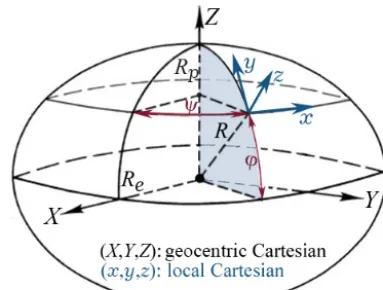
com-Figure 1.Local and geocentric Cartesian coordinate systems.
pare the spatial distribution of particles washed ashore with the locations where MH370 fragments were found.
2.1 Model description 2.1.1 Assumptions
In the context of this study it was assumed that a particle was subjected to the drag forces induced by water and wind. Parti-cles were assumed to be non-inertial. Impacts of the Coriolis force, Stokes drift, waves, decay, and sinking were neglected (e.g. Kraus, 1972; Al-Rabeh et al., 2000). In the local coordi-nate system(x, y), where the axesxandycorrespond to the local west-to-east and south-to-north directions respectively (Fig. 1), the location(xi, yi)of theith particle was described by Langevin’s equation (DHI, 2009):
dxi
dt =ui+D(t, xi, yi)ζ,
dyi
dt =vi+D(t, xi, yi)ξ, (1)
where(ui, vi)is the average (deterministic) velocity of the ith particle in the local coordinate system,Dis the turbulent diffusion term, andζ, ξare the random numbers, as detailed in Sect. 2.1.3 through 2.1.5.
2.1.2 Coordinate systems
On the one hand, the velocity of a particle and random walk are formulated in the local coordinate system, where the axis
z is normal to the Earth surface. On the other hand, the large study domain dictates the necessity to properly take into consideration the Earth curvature. To perform numer-ical integration of the governing equations in the geocen-tric Cartesian coordinate system(X, Y, Z)depicted in Fig. 1, where the Earth surface is approximated by WGS 84 ellip-soid with the polar and equatorial axes radiiRp=6 356 752 and Re=6 378 137 m respectively, the transformations of coordinates and velocity vectors are required.
The Cartesian coordinatesX,Y, andZ of a point on the surface of the ellipsoid described by the longitudeψand geo-centric latitudeϕcan be formulated as
X=Rcosϕcosψ, Y=Rcosϕsinψ, Z=Rsinϕ, (2) where
R= ReRp
q
(Rpcosϕ)2+(Resinϕ)2
is the distance between this point and the centre of the ellip-soid, as follows from the ellipse equation
(Rcosϕ)2 R2
e
+(Rsinϕ) 2 R2
p
=1.
It should be noted that the backward transformation is re-quired to extract and interpolate surface current and wind data at a given location. Respective trigonometric transfor-mations involve solving a fourth-degree polynomial equa-tion.
The unit vectors −→L, −→M, and −→N, which define the di-rections of the axes x, y, and z of the local coordinate system (Fig. 1), are introduced to obtain velocity compo-nents in the geocentric system. The outward unit vector
− →
N = {NX, NY, NZ,}normal to the surface of the ellipsoid is formulated according to Korn and Korn (1968):
− → N = n ∂X ∂ψ, ∂Y ∂ψ, ∂Z ∂ψ o
×n∂X ∂ϕ, ∂Y ∂ϕ, ∂Z ∂ϕ o n ∂X ∂ψ, ∂Y ∂ψ, ∂Z ∂ψ o
×n∂X ∂ϕ, ∂Y ∂ϕ, ∂Z ∂ϕ o H⇒
NX= 1 p
1+µ2 cosϕ
−µsinϕ cosψ,
NY = 1 p
1+µ2 cosϕ
−µsinϕsinψ,
NZ= 1 p
1+µ2 sinϕ+µcosϕ
,
whereµ=R2R 2 e−Rp2 R2
eR2p
cosϕ sinϕ. (3)
The direction of the axisxis defined by the unit vector−→L:
− →
L = {LX, LY, LZ} = {−sinψ,cosψ,0}. (4) Equations (3) and (4) allow expressing the unit vector
− →
M= {MX, MY, MZ}collinear with the axis y in the form of the vector product−→M=−→N ×−→L, so that its components are
MX= − 1 p
1+µ2 sinϕ
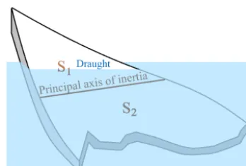
Figure 2.Schematic representation of a thin floating object.
MY = − 1 p
1+µ2 sinϕ
+µcosϕ sinψ,
MZ= 1 p
1+µ2 cosϕ
−µsinϕ. (5)
Therefore, a velocity vector, the components of which are
{u, v,0}in the local system, has the following components in the geocentric Cartesian system:
U= −usinψ−v p 1
1+µ2(sinϕ+µcosϕ)cosψ, V = ucosψ−v p 1
1+µ2(sinϕ
+µcosϕ)sinψ,
W = v p 1
1+µ2(cosϕ
−µsinϕ) . (6)
Hence, Langevin’s Eq. (1) can be formulated in the geo-centric Cartesian system as follows:
dXi
dt =U (ui, vi, ψi, ϕi)+D (LXζ+MXξ ),
dYi
dt =V (ui, vi, ψi, ϕi)+D (LYζ+MYξ ),
dZi
dt =W (ui, vi, ψi, ϕi)+D (LZζ+MZξ ),
(7)
where the relations between the longitudeψi and geocentric latitudeϕi of particle’s location and its geocentric Cartesian coordinatesXi,Yi,Zi are given by Eq. (2); the transforma-tion of the velocity components is given by Eq. (6); and the local velocity components ui, and vi are defined from the balance of the deterministic forces.
2.1.3 Deterministic terms
The mathematical description of the dynamics of a float-ing object is not a trivial problem due to the variety of pro-cesses and phenomena in a near-surface layer, such as surface waves, Stokes drift, flow–object interaction, buoyancy, and stratification (e.g. Kraus, 1972). Such an object is subjected
to the dynamic pressure and shear stress forces due to the ac-tion of the water and air; its steady-state orientaac-tion depends on its buoyancy characteristics and the moments of forces around its principal axes of inertia. Denoting−→ui =(ui, vi) the deterministic velocity of theith particle representing a floating object in the local coordinate system and neglecting the Coriolis force, its motion in the local horizontal plane is described by the following equation:
mi d−→ui
dt = −−→
Fw,i+ −−→
Fa,i, (8)
wheremi is the mass of the object and −−→
Fw,i and −−→
Fa,i are the average forces caused respectively by water and air flows around the object. The same formulation of these forces as applied in Daniel et al. (2002) and Breivik et al. (2011) to study drift of ship containers was adopted in this study, al-though justification for thin nearly horizontally floating ob-jects (Fig. 2) could be slightly different. According to the the-ory of a turbulent boundary layer (e.g. Kraus, 1972; Gandin et al., 1955), vertical velocity profiles of the water and air exhibit a logarithmic dependence on the distance from the surface
U (z)=u∗ κ ln
|z| z0 ,
whereu∗ is the friction velocity,κ=0.41 is von Kármán’s constant, andz0is roughness, where the surface is assumed to be non-moving at z=0. The turbulent shear stresses
τ{w,a}=ρ{w,a}u2∗{w,a}, whereρ{w,a} is the density of the wa-ter or air, remain constant through this layer. Hence, the shear stresses acting on the top and bottom surfaces of a thin float-ing object can be considered proportional to
−→
uw− − → u 2 and − →
ua− − →
u 2
, where−u→w= −→
uw(xi, yi, t ) and − →
ua= − →
ua(xi, yi, t ) are the current and wind velocities at the location of the ob-ject at a certain reference depth and height (the typical refer-ence height for wind is 10 m above the surface). The dynamic pressures can also be considered proportional to the squared relative velocities of water and air but at some other repre-sentative distances. Bearing in mind the logarithmic velocity profile, the latter would also be proportional to
−→
uw− − → u 2 and − →
ua− −→
u 2
respectively. Therefore, if the drag forces are collinear with the respective relative velocities of the water and air, the same formulation as in Daniel et al. (2002) would also be applicable for thin objects:
−−→
Fw,i= 1
2CDw,iSw,i ρw
−→
uw− − → ui −→
uw− − →
ui, −−→
Fa,i = 1
2CDa,i Sa,i ρa
− →
ua − − → ui − →
ua− − →
ui
, (9)
ob-ject, CDa,i and Sa,i are the air drag coefficient and corre-sponding reference area of the part exposed to the air,ρwand ρaare the water and air densities. Furthermore, Breivik et al. (2011) argued that wave drift forces on small objects (less than 30 m) decay rapidly, and they can be neglected com-pared to wind forces when the wave length is more than 6 times the dimensions of a floating object.
It should be noted that composite materials are usually light-weight structures. For example, the recovered flaperon is approximately 1.6 m×2.4 m×0.25 m in size and 50 kg in weight. Bearing in mind that the typical values of the min-imum drag coefficient CDa for airfoils are in the range of 0.02 to 0.05 with respect to their surface areas, it is easy to show that the drag forces acting on such a fragment of the air-craft would normally be much larger compared to the inertial term in Eq. (8), and hence the latter can be approximated by the balance equation:
−−→
Fw,i= − −−→
Fa,i. Using Eq. (9), the latter yields
1
2CDw,iSw,iρw
− →
ui−−u→w(xi, yi, t )
−→
ui−−u→w(xi, yi, t )
=
−1
2CDa,iSa,iρa
− →
ui− − →
ua(xi, yi, t )
−→ ui−
− →
ua(xi, yi, t )
. (10) It is easy to see that the solution of Eq. (10) is
−→
ui =(1−αi) −→
uw(xi, yi, t )+αi − →
ua(xi, yi, t ), (11) where the scalarαi (leeway factor) is
αi=
p
CDa,iSa,i ρa p
CDa,iSa,i ρa+pCDw,iSw,i ρw
. (12)
For a thin horizontally floating object, which has equal ar-eas of the surface exposed to seawater and air (Sa=Sw) and which is characterised by equal drag coefficientsCDa=CDw, the leeway factor isα≈3.33 %. This theoretical value is in a good agreement with the experimental data for the flaperon (3.29 %) estimated by the DGA in the hydrodynamic engi-neering test facility centre in Toulouse (Daniel, 2016). For a 70 %-submerged cube, this formulation yields α=2.2 % assuming the dominance of the dynamic pressure acting on the lateral faces and being also in a good agreement with the experimental factor of 2 % (Breivik et al., 2011).
In two of the four considered models (Sect. 2.2), where the force induced by relative wind was not collinear with its di-rection, a modified formulation was used instead of Eq. (11):
−→
ui =(1−αi) −→
uw+αi
cosθ −sinθ
sinθ cosθ
−→
ua, (13)
whereθis the drift angle and is positive counter-clockwise.
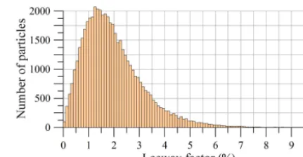
Figure 3.Assumed distribution of leeway factors across an ensem-ble (constant in time for an individual particle).
2.1.4 Random leeway factor model
In contrast to earlier studies (e.g. Daniel, 2016; Pattiaratchi and Wijeratne, 2016; Griffin et al., 2017), an attempt was made in this work to take into consideration the variety of leeway factors, which describe random shapes and flota-tion characteristics of individual fragments generated by the crash. For this purpose, in one of the four considered types of ensembles (Sect. 2.2) particles were described by random leeway factors. It was assumed that these particles repre-sented partially submerged thin objects of irregular shapes floating in slightly tilted orientations (Fig. 2). For the sake of simplification, it was assumed that the drag coefficients for the air and water are equal (CDa,i=CDs,i). Then, according to Eq. (12), only the knowledge of the ratio of respective ar-eask=Sa,i/Sw,i is required to estimate the leeway factor:
αi= √
ρa/ρw √
ki 1+√ρa/ρw
√ ki
. (14)
In the context of this study it was assumed that dimensions of individual objects are log-normally distributed. Further-more, it was assumed that the principal axis of inertia of the object splits it into two parts, areas of which are also log-normally distributed, so that
ki=
γiSi,1 Si,2+(1.0−γi)Si,1
,
wherelnSi,1,lnSi,2 ∈N(µ, σ2)and γ∈ [0,1] is an in-dependent random parameter to account for the draught of the object (0 – fully submerged; 1 – the centre of gravity is at the water surface). Hence the logarithm of the ratio ln(S1/S2)=lnS1−lnS2∈N(0,2σ2) is also normally dis-tributed, with a mean of 0. Here the property was used that the sum of two independent normally distributed random variables is also normally distributed, with its mean being the sum of the means and its variance being the sum of the two variances (Eisenberg and Sullivan, 2008). Hence, the ratio
this class of simulations (hereafter referred to as the “random leeway” model) is depicted in Fig. 3. A random leeway factor assigned to a particle in ensemble was constant in time. 2.1.5 Numerical realisation and random walk
The whole integration interval was split into time steps of
1t=15 min. Similarly to the DHI (2009) particle tracking model, the integration of the system of equations (Eq. 7) for each particle over the time step1twas comprised of the two stages, namely the deterministic and the stochastic one:
−→
Xi(t+1t )=−X→i(t )+ t+1t
Z
t − →
U(ui, vi, ψi, ϕi)dt,
−→
Xi(t+1t )= −→
Xi(t+1t )+ − →
δi(. . .),
where −X→i = {Xi, Yi, Zi} is the location of the ith parti-cle;
− →
Xi is the intermediate location prior to the superposi-tion of the random displacement−→δi(. . .);
− →
U(ui, vi, ψi, ϕi)=
U (. . .), V (. . .), W (. . .) is the velocity of the particle. Un-like the DHI (2009) model, which uses the first-order dis-cretisation method to integrate deterministic terms, the fifth-and sixth-order Runge–Kutta method was used in this work utilising FORTRAN libraries to ensure that particles remain on the ellipsoid’s surface with sufficient accuracy. During the integration, input current and wind data were bilinearly inter-polated in space and linearly in time.
The vector−→δi(. . .)corresponds to a numerical solution for the diffusivity term of the Langevin Eq. (1). It was treated as a random displacement in thexyplane locally tangential to ellipsoid’s surface. Its componentsδx andδy in the local coordinate system are the random values from the trimmed two-dimensional Gaussian distributionN2:
δx=σLζ, δy=σLξ, (15)
where {ζ, ξ} ∈N2(0,1) are the random numbers and the standard deviation of the turbulent dispersionσL=
√
2D 1t
is assumed to be a function of the horizontal eddy diffusivity coefficientD=D(t, ψi, ϕi). Such a relation betweenDand σLwas first established by A. Einstein in 1905, who studied diffusion associated with Brownian motion, and since then it was adopted in a variety of random walk models (e.g. DHI, 2009; Jansen et al., 2016). In this study trimming was im-posed to discard values δx andδy that resulted in displace-ments exceeding 10 km distance over the time step1t. If this criterion was violated, the next pair of random valuesδxand δywas computed. The distance of 10 km was selected as the representative resolution of the ocean circulation model HY-COM, used as a source of the surface current velocity data (see Sect. 2.2.2).
In contrast to Jansen et al. (2016), who applied the con-stant eddy diffusivity coefficientD=2 m s−1, in this work Dwas computed according to the well-known Smagorinsky (1963) parameterisation, applied in various ocean circulation models (e.g. Blumberg and Mellor, 1987; DHI, 2009):
D=κ1x1y
s ∂u
∂x
2
+1
2 ∂u
∂y+ ∂v ∂x
2
+
∂v
∂y
2
, (16)
whereκ=0.1 is the constant coefficient (a typical range is from 0.1 to 0.2 according to Blumberg and Mellor, 1987), and1xand1yare the horizontal dimensions of the numer-ical grid cell, applied for the discretisation of the velocity field. A discrete approximation of Eq. (16) was used to esti-mate the eddy diffusivity coefficientD, with subsequent bi-linear interpolation in space and bi-linear interpolation in time at the actual locations of particles.
In the geocentric Cartesian coordinate system the ran-dom displacement translates into the 3-D vector −→δi =
δXi, δYi, δZi , components of which are
δXi=LXδx+MXδy, δYi =LYδx+MYδy,
δZi =LZδx+MZδy. (17)
Such a displacement in the tangential plane causes a parti-cle to move away from the surface of the ellipsoid. However, due to the imposed limitation on the distance, the elevation of the particle does not exceed 8 m after superposition of the random walk. Thus, particle elevations were forced to zero after applying the random walk procedure at each integration time step, while preserving longitudes and latitude.
A Box and Muller (1958) transform was used to obtain a pair of pseudo-random numbers{ζ, ξ} ∈N2(0,1):
ζ= √
−2 lnτ cos(2π ω), ξ = √
−2 lnτ sin(2π ω), (18) whereτ and ω are the two pseudo-random numbers from the interval(0,1]. To obtain τ andω, the use was made of the generator developed by Marsaglia and Zaman (1987), claimed to have the period of 2144.
Close to a shore, flow velocity was linearly interpolated between zero and velocity in the adjacent cell of the numeri-cal grid of HYCOM. If a particle moved onshore as a result of wind action or random walk, all the subsequent forcing acting on such a particle was nullified, so that it remained at the location where it beached. No specific properties of the shores (e.g. type, slope) or contributing factors such as waves, tides, or storm surges, were considered.
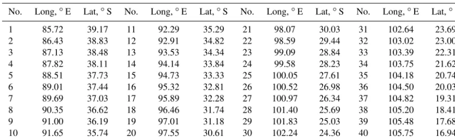
Con-Table 1.Longitudes and latitudes of the origins preselected for screening
No. Long,◦E Lat,◦S No. Long,◦E Lat,◦S No. Long,◦E Lat,◦S No. Long,◦E Lat,◦S 1 85.72 39.17 11 92.29 35.29 21 98.07 30.03 31 102.64 23.69 2 86.43 38.83 12 92.91 34.82 22 98.59 29.44 32 103.02 23.00 3 87.13 38.48 13 93.53 34.34 23 99.09 28.84 33 103.39 22.31 4 87.82 38.11 14 94.14 33.84 24 99.58 28.23 34 103.75 21.62 5 88.51 37.73 15 94.73 33.33 25 100.05 27.61 35 104.18 20.74 6 89.01 37.44 16 95.32 32.81 26 100.52 26.98 36 104.50 20.03 7 89.69 37.03 17 95.89 32.28 27 100.97 26.34 37 104.82 19.31 8 90.35 36.62 18 96.46 31.74 28 101.40 25.69 38 105.20 18.41 9 91.00 36.19 19 97.01 31.18 29 101.83 25.03 39 105.48 17.68 10 91.65 35.74 20 97.55 30.61 30 102.24 24.36 40 105.75 16.94
ducted tests have shown that the maximum errors in the el-evation of a particle, which resulted from a single forward– backward conversion of the coordinates, were of the order of 0.5 mm using the extended precision compared to 0.5 m using the double-precision arithmetic.
2.2 Model set-up
Four models with respect to the leeway factor and drift angle of particles in an ensemble were considered:
– a leeway factor of 3.29 %; zero drift angle;
– a leeway factor of 3.29 %; drift angle of 18◦to the left; – a leeway factor of 2.76 %; drift angle of 32◦to the left; – random leeway factor; zero drift angle.
All the ensembles released at various locations were iden-tical with respect to the properties of particles in these ensem-bles. Each ensemble comprised 50 000 particles, the same as in Pattiaratchi and Wijeratne (2016). The second and third models focused specifically on the flaperon path: respective settings corresponded to the flotation characteristics estab-lished by the DGA (Daniel, 2016). The fourth model aimed to achieve a more realistic representation of the flotation characteristics of the debris generated by the crash by assign-ing random leeway factors (fixed in time) to the particles of an ensemble; all the 40 ensembles (Sect. 2.2.1) were identical in terms of the particles they were comprised of.
2.2.1 Screened locations
The study domain extended from 20 to 140◦E, 55◦S to 15◦N. Integration was performed from 8 March 2014 to 31 December 2016 inclusive. The locations of the 40 hypothet-ical debris origins are summarised in Table 1 and indicated in Fig. 4. The coordinates of these locations were estimated from the burst time offset (ATSB, 2015) of the last “hand-shake” 00:19, assuming that the aircraft was at the altitude of 10 km.
2.2.2 Model forcing and SST data
The following datasets were used in this study for the model forcing and temperature analysis:
– Surface currents were extracted from the Hy-brid Coordinate Ocean Model, a data-assimilative isopycnal-sigma-pressure coordinate ocean cir-culation model (Chassignet et al., 2007). Spa-tial resolution: 0.08◦×0.08◦; temporal resolu-tion: daily. The HYCOM consortium is a multi-institutional effort sponsored by the National Ocean Partnership Program (https://hycom.org/, last ac-cess: 17 May 2018); data are available at ftp: //ftp.hycom.org/datasets/global/GLBa0.08_rect/data/ (last access: 17 May 2018).
– Wind velocitieswere extracted from the Global Data As-similation System, provided by the Air Resources Lab-oratory (ARL) of the U.S. National Oceanic and At-mospheric Administration (NOAA). Spatial resolution: 1◦×1◦; temporal resolution: 3 h. Further details are available at http://www.ready.noaa.gov/gdas1.php (last access: 17 May 2018); archived data in a proprietary format are available at ftp://arlftp.arlhq.noaa.gov/pub/ archives/gdas1 (last access: 17 May 2018).
– SST data were sourced from a Group for High Res-olution Sea Surface Temperature (GHRSST) Level 4 MUR Global Foundation Sea Surface Tempera-ture Analysis, a product developed by the Jet Propul-sion Laboratory under NASA MEaSUREs program (JPL, 2015). Spatial resolution: 0.011◦×0.011◦; tem-poral resolution: daily. Detailed information on this data is available at https://mur.jpl.nasa.gov/ (last ac-cess: 17 May 2018) and https://podaac.jpl.nasa.gov/ dataset/JPL-L4UHfnd-GLOB-MUR (last access: 17 May 2018).
avail-Figure 4.Locations of the selected hypothetical origins on the seventh arc and snapshots of the sea surface temperatures.
Figure 5.Snapshots of particle ensembles originating from several locations (indicated with corresponding colours of ensembles) on 30 March for two models and the areas surveyed by 2 April. Sources of the aerial search maps and photograph: JAAC (2014), AMSA (2014).
able from the National Oceanic and Atmospheric Adminis-tration’s Global Drifter Program (Eliot et al., 2016), which passed through the study domain from March 2014 until De-cember 2016 (a total of 820 801 samples) have shown rms errors of 26.6 and 26.0 cm s−1for the easterly and northerly components respectively. However, further analysis is re-quired to understand the contribution of wind to these errors (e.g. Griffin et al., 2017, suggest that the average leeway fac-tor of the GDP buoys is around 1.2 %) and, more importantly, how they can affect modelling accuracy, particularly with re-gard to whether they are stochastic or systematic.
3 Results
3.1 Efficacy of the aerial search
An extensive aerial search for MH370 debris, which lasted from 18 March to 27 April 2014, (e.g. JAAC, 2014; AMSA, 2014), failed to find any debris relevant to MH370. Although some suspected objects were observed on 28–31 March (AMSA, 2014), such as a rectangular object photographed from the specialised Royal New Zealand Airforce (RNZAF) Orion P3K survey aircraft (Fig. 5), subsequent attempts to recover them were unsuccessful.
sev-Figure 6.The five largest daily coverages during the aerial search (in descending order: black, red, yellow, green, and blue bars).
Table 2.Estimated maximum daily coverage (%), respective date of its occurrence (2014), and cumulative coverage (%) for each screened ensemble based on the proposed random leeway factor model.
No. Max. Cumu- Date No. Max. Cumu- Date No. Max. Cumu- Date No. Max. Cumu- Date
daily lative daily lative daily lative daily lative
1 90.7 91.9 Mar 19 11 24.9 25.1 Apr 01 21 30.4 114.1 Mar 31 31 25.8 132.9 Apr 04
2 19.8 37.2 Mar 19 12 10.7 16.9 Apr 01 22 45.1 279.0 Mar 28 32 66.7 419.3 Apr 04
3 18.6 18.6 Mar 18 13 66.0 107.0 Apr 01 23 28.6 116.1 Apr 02 33 53.4 137.4 Apr 05
4 4.3 4.3 Mar 19 14 36.8 62.6 Apr 01 24 43.1 192.3 Mar 28 34 63.1 254.8 Apr 05
5 13.6 13.6 Mar 19 15 71.1 142.0 Mar 31 25 34.9 199.1 Mar 28 35 62.4 234.6 Apr 05
6 0.4 0.4 Mar 19 16 67.3 160.7 Mar 31 26 19.5 136.2 Mar 29 36 42.3 138.9 Apr 03
7 <0.1 <0.1 Mar 19 17 65.3 244.3 Apr 01 27 10.5 68.8 Apr 20 37 0.3 0.6 Apr 05
8 0 0 – 18 61.7 295.1 Mar 29 28 12.5 46.3 Apr 18 38 0.2 0.6 Apr 05
9 <0.1 <0.1 Apr 01 19 50.0 256.8 Mar 29 29 46.4 126.3 Apr 13 39 0 0 –
10 0.8 0.8 Apr 01 20 68.3 245.1 Mar 29 30 19.0 100.8 Apr 04 40 0 0 –
enth arc on 28 March and 5 April are depicted in Fig. 5 for the random and constant 3.29 % leeway factor models. An ani-mation, which shows computed daily positions of these en-sembles and search areas, is presented in the Supplement S1. As seen, the leeway factor had a significant influence on the dispersion, which was notably more intense for the ensem-bles that comprised particles of various leeway factors. Fur-thermore, the difference in the leeway factors could presum-ably explain the failed attempts to track suspected objects with the help of deployed buoys. It is worth noting that the aerial survey appears to be rather inefficient for the objects characterised by the leeway factor of 3.29 % (such as the flap-eron), which originated from the locations around 30◦S or from the segment from 25.5 to 28◦S of the seventh arc.
To better understand reasons contributing to the aerial search failure, daily efficacies of the search were analysed in terms of the percentagesEj,kof particlesij,kof eachjth ensemble, which were in the search areak on thekth day of the search:
Ej,k= 1
N
X
k
ij,k !
×100 %, (19)
whereN=50 000 is the number of particles per ensemble. Respective areask were obtained by digitising maps pub-lished in AMSA (2014) and JAAC (2014) portals.
As the value of the maximum single-day coverage max
k Ej,kcould be downplayed by other factors affecting de-tection capability, such as poor weather conditions, the five largest estimated daily coverages of particle ensembles are presented in Fig. 6 for the random and constant 3.29 % lee-way factor models versus the origin’s latitude along the sev-enth arc. The maximum single-day coverage, date of its oc-currence, and cumulative coverage over the entire duration of the search campaign are summarised in Table 2 for each screened ensemble based on the proposed random leeway factor model. The cumulative coverages were defined as the sumP
kEj,kof daily ensemble coverages over the duration of the search campaign. It can be viewed as an additional selection criterion of a more likely origin when peak daily coverages are similar, such as in the case of ensembles no. 21 and no. 25 (Table 2).
lower if the crash site was located between 25.5 and 27.5◦S. In particular, for the origins no. 27 and no. 28, the maxi-mum coverages of approximately 10 % occurred more than 6 weeks after the crash, which is a rather low figure bearing in mind that decay and sinking processes were not taken into consideration. A relatively poor coverage is also noted for the origins no. 21 and no. 23.
Interestingly, a rectangular object spotted from RNZAF Orion P3K on 28 March was in the area, where some de-bris originating from the location no. 21 (98.07◦E, 30.03◦S) could be expected according to the random leeway model (Fig. 5). Furthermore, the timing of the peak coverages (28– 31 March; see Table 2) for the debris originating from this and neighbouring locations is consistent with the dates when a number of floating objects were detected there.
3.2 SST along the path of the flaperon
One of the major goals of this study is to address a ques-tion whether the ambient water temperatures along modelled particle tracks could match the temperature variation derived from the biochemical analysis of the barnacles attached to the flaperon (De Deckker, 2017) and, if yes, whether this infor-mation could help to further refine the search area. Therefore, those particles were of interest which satisfied the following two conditions:
– A particle must have arrived at the St-André beach, a place where the flaperon was found (assumed coordi-nates 55.67◦E, 20.93◦S), by 29 July 2015.
– The ambient SST at a particle’s location should have first exceeded 24◦C, then dropped down below 18◦C, and then risen up again to 25◦C or higher.
Due to the inherent uncertainty in the temperature estima-tions based on the barnacle analysis, a score-based function
S was introduced to identify those particles which approxi-mately satisfied the two aforementioned conditions:
Si =Si,d Si,θ. (20)
Here the termSi,d=exp(−0.5di2/dref2 )is responsible for the first condition above; di=di(ψi, ϕi)is the ground dis-tance between theith particle location on 29 July 2015 and the St-André beach;dref=50 km is the reference distance, which was chosen to be the approximate linear dimension of La Réunion. The termSi,θ responsible for the second condi-tion, was formulated in the following way:
Si,θ=
Si,θ1+Si,θ2+Si,θ3
3 , if∃{t1, t2, t3}∈ [Ts, Te] : max
0≤t≤t1θi(t )
≥23◦C,
min
t1≤t≤t2θi(t )≤19 ◦C, max
t2≤t≤T
θi(t )≥24◦C,
0 otherwise,
(21)
whereθi(t )is the SST at theith particle location at the time t(Ts≤t≤Te, whereTs andTecorrespond to 8 March 2014 and 29 July 2015 respectively) and
Si,θ1=min(max(max 0≤t≤t1θi(t )
−23, 0), 1), Si,θ2 =min(max(19−min
t1≤t≤t2
θi(t ), 0), 1), Si,θ3=min(max(max
t2≤t≤Tθi(t )
−24, 0), 1).
The purpose of such a formulation Eq. (20) is to relax the selection criteria and avoid discontinuities by assigning a positive score to a particle even if it did not arrive precisely at the St-André beach or if it did not strictly satisfy the tempera-ture condition (the tolerance allowing for a positive score was set to 1◦C). As a result, the maximum score a particle could receive was 1. If a particle arrived at La Réunion before 29 July, it was still assigned a positive score. If a particle was lo-cated at a distance greater than 152 km from St-André beach on 29 July, it could not receive a score higher than 0.01. If the SST at a particle’s location never reached 23◦C or never dropped below 19◦C after that, such a particle received a 0 score.
The percentages of particles in ensembles which received scoresS >0.01 vs. origin’s latitude along the seventh arc are shown in Fig. 7 for all the four model set-ups, together with the normal distribution fitting. As seen, for the leeway factors and non-zero drift angles of the flaperon determined by the DGA (Daniel, 2016), the segment centred at 28.2±3◦ ap-pears to be the most likely area where the flaperon began its journey. A fraction of particles in the two other models (char-acterised by zero drift angle), which satisfied the two con-ditions, could reach a surprisingly high value of 1 %; how-ever, both the random leeway factor and constant 3.29 % lee-way factor models indicated the peak fitted probabilities at 30.8 and 31.9◦S respectively. The screened origins south of 36.5◦S or north of 20◦S are deemed to be unlikely starting locations of the flaperon, as none of the four models pdicted a notable percentage of particles meeting the two re-quirements above for the corresponding ensembles.
Examples of the first six particle tracks, which received the highest scoresS, are depicted in Fig. 8 for the scenario corre-sponding to the leeway factor of 3.29 % and drift angle 18◦to the left, starting from the origin no. 23 (99.09◦E, 28.84◦S). All these particles received the scoresSi>0.83, and they ar-rived at La Réunion between 17 June (black track) and 17 July (yellow track) 2015. As seen, the two main reasons for the drop in the ambient water temperature from 23–25◦C to as low as 16◦C are as follows:
– seasonal cooling of the water surface (see comparison of the SSTs on 8 March and 8 June 2014 in Fig. 4); – entrapment in counter-clockwise eddies, which could
Figure 7.Percentages of particles satisfying distance and temperature criterion with the scoreS >0.01 (LW: leeway factor; DA: drift angle).
Figure 8.Sample tracks and temperatures for the six particles of ensemble no. 23 (leeway 3.29 %; drift angle 18◦).
3.3 Beached debris distribution
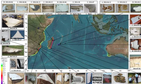
A total of 27 possibly relevant and confirmed fragments of 9M-MRO were recovered in La Réunion, Mauritius, Ro-drigues Island, Madagascar, Mozambique, South Africa, and Tanzania as of April 2017 according to the MSIT (2017); none was ever found in Australia, although a suspected ob-ject, the unopened towelette bearing the MAS logotype, was discovered at Thirsty Point. The distribution of the debris
found offers a useful insight into the possible location of the crash site (e.g. Jansen et al., 2016; Pattiaratchi and Wijer-atne, 2016; Griffin et al., 2017), although no consensus has been reached to date with regard to the origin. Similarly to the aforementioned studies, an effort was made in this study to analyse the spatial distribution of the fragments washed ashore.
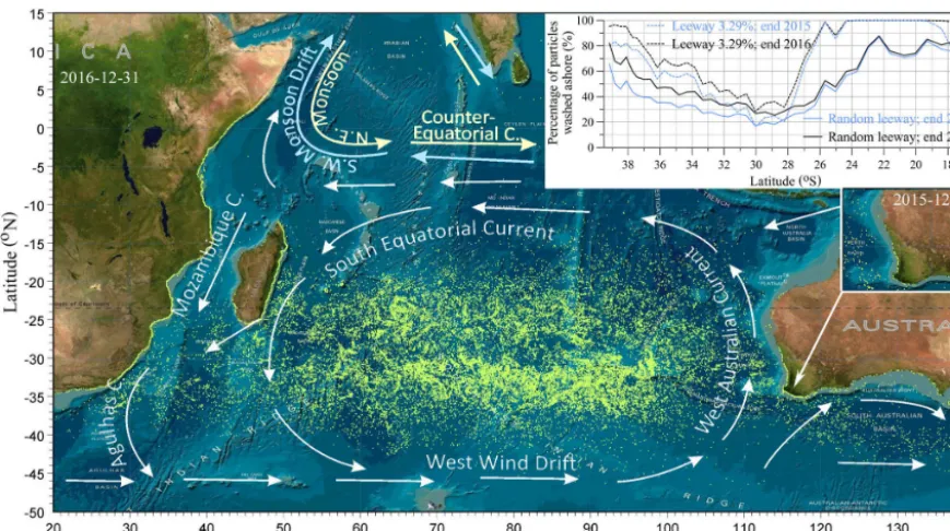
lee-Figure 9.Snapshot of particle locations on 31 December 2016 (random leeway model; origin no. 23) and percentages of particles washed ashore.
Figure 10.Expected number of objects to be found in several countries by 31 December 2016 vs. origin’s latitude.
way model, origin no. 23. Corresponding animation S2a is included in the Supplement. Considerable beaching of par-ticles of this ensemble was modelled in Africa, Madagascar, La Réunion, and Mauritius, but it was negligible in Australia. The total fractions of particles landed by the end of 2015 and 2016 are shown in the top right corner for all the screened origins, both the random and constant 3.29 % leeway factor models. This result is, in part, due to the West Australian Cur-rent, which entrains large percentages of particles from the northern and southern origins (see animations S3 and S4), while most of particles from the middle of the screened
seg-ment of the seventh arc remain trapped in the Indian Ocean Gyre.
Figure 11.Expected along-shore concentration of beached MH370 fragments from the hypothetical origin no. 23 to be found by the end of 2016.
Table 3.Sensitivity of the percentages of particles washed ashore by the end of 2016 to the number of particles in ensembles (origin no. 23).
Number
of
particles
Andaman
Islands
Australia India Indonesia Ken
ya
Madag
ascar
Mauritius Mozambique La
Réunion
Somalia South
Africa
Sri
Lanka
T
anzania
Ov
erall
beached
Escaped
domain
50 000 0.078 0.854 0.022 0.048 0.300 12.166 1.966 3.068 2.338 0.272 1.946 0.090 0.952 25.430 0.724 500 000 0.090 0.866 0.037 0.037 0.329 12.163 1.976 3.097 2.438 0.289 1.908 0.087 0.977 25.703 0.744
nine objects in Tanzania, and three objects in Kenya, should the origin be south of 35◦S. At least one fragment could be expected in Sri Lanka and several in Kenya and Tanzania for the origins north of 23◦S. The best matching segment of the seventh arc is located approximately between 26.5 and 31◦S. In particular, the ratio of the percentages of particles beached in Mozambique to those in South Africa was in the range of 1.4 to 1.7, being in a good agreement with the actual ratio of 6:5.
To estimate the along-shore concentration of MH370 ob-jects expected to be found by a certain time, the two-dimensional Gaussian smoothing filter was first applied to obtain a smoothed concentration of beached particles:
P (ψ, ϕ)= 1
2π dref2 M X
i=1
exp −d 2
i(ψ, ϕ, ψi, ϕi) 2dref2
!
,
wheredi is the ground distance between theith beached par-ticle and the location of interest (ψ, ϕ), dref=5 km is the size of the smoothing filter, andMis the number of beached particles. To compute the along-shore density distribution of objects expected to be found, this function was numer-ically integrated over a relatively narrow band-shaped area
Figure 12.Arrival times of particles to the proximity of Thirsty Point (Australia) during 2014 and Mossel Bay (South Africa).
NSA=5 to the number of particles landed in South Africa MSA:
dN
ds ≈ NSA MSA
1
1si Z Z
i
P (ψ, ϕ)d.
An example of the concentration of objects estimated in this way is shown in Fig. 11 for the ensemble released from origin no. 23 (random leeway model); concentrations for all the other studied origins are presented in Fig. S5 and anima-tion S5. As seen, the locaanima-tions of the elevated concentraanima-tions are in a fairly good agreement with the locations where the fragments were found, except Rodrigues Island, which was not properly resolved by HYCOM. More fragments could be expected in Tanzania at 7.0 and 8.2◦S.
Screening of origin no. 23 has revealed that the elevated concentration near Cape Leeuwin in Australia is due to the beaching which mainly occurred in 2016. During 2014–2015 notable arrival of particles from this origin to Australia took place only around Windy Harbour and Thirsty Point, where the unopened MAS towelette was found on 2 July 2014 (as-sumed coordinates 115.3◦E, 31◦S). A detailed analysis has shown that 8 particles of the respective ensemble landed near Thirsty Point during 8–11 July, and 10 more particles arrived before 28 July. All the first 8 particles were characterised by relatively low leeway factors ranging from 0.1 to 0.4 %. This suggests a systematic feature rather than a random occur-rence. Systematic arrival of particles from the origins north of 27◦S or south of 31◦S was not predicted earlier than in the last week of July, as seen in Fig. 12.
Figure 12 also shows the arrival times of particles to Mos-sel Bay in South Africa, where the engine cowling fragment was found. Being the fourth object found, it had covered a long distance over a relatively short time interval. The mod-elling has shown the possibility of the sporadic arrival of high-windage particles to Mossel Bay as early as February 2015, but systematic arrival was predicted only for March– May 2016, consistent with the discovery date.
To understand the sensitivity of the results presented in this section to the number of particles in ensembles, a
nu-merical experiment was conducted using 500 000 particles for origin no. 23 in the random-leeway factor model (see an-imation S2b). The results of this experiment (Table 3) in-dicate that the use of 50 000 particles is sufficient to obtain fairly reliable statistics, and a further increase in the number of particles would unlikely be beneficial.
4 Conclusions
The drift study of MH370 debris was conducted by means of numerical modelling using a forward particle tracking tech-nique. A total of 40 hypothetical locations of the crash site along the seventh arc were screened. Three major aspects were considered: (1) the efficacy of the aerial search; (2) am-bient water temperatures along the path of the flaperon to La Réunion; (3) the spatial distribution of the debris washed ashore.
The governing equations were numerically integrated in the geocentric Cartesian coordinate system, where the Earth surface was approximated by the WGS 84 ellipsoid. Four models with respect to the leeway factors and drift angles were considered, including a proposed model of random dis-tribution of the leeway factors of particles in an ensemble.
The obtained results indicate the significance of the lee-way factor in all the three aspects considered. In addition to the uncertainties in the model forcing, assumptions, and sim-plification, a judgment about the most likely location of the crash site depends on weights assigned to the aerial search, the accuracy of the barnacle biochemical analysis, and the probability of fragments not only being washed ashore but also being recovered and reported. While it does not appear to be possible to confidently point out the location of the crash site based on the drift study alone, a few observations can be made with regard to various segments of the seventh arc:
– 34.5 to 36◦S.While corresponding areas were poorly surveyed during the aerial search, considerable beach-ing could be expected in several countries where no fragments were found, particularly in Australia. – 30.5 to 34.5◦S.Excellent aerial coverage of the debris
cloud originating from this segment makes the crash site unlikely to be located within it.
– 25.5 to 30.5◦S.Consistency with the barnacle temper-ature analysis; elevated concentration of beached parti-cles, where the fragments of 9M-MRO were found; sev-eral “gaps” in the aerial search; floating objects detected on 28–31 March; possible consistency with the early ar-rival of the MAS towelette at Thirsty Point.
– North of 25.5◦S.Inconsistency with the distribution of the debris washed ashore; incompatibility with the bar-nacle temperature analysis; good aerial coverage of the areas corresponding to the origins from 20 to 25◦S. Summarising all the above, the most likely area of the crash site appears to be between 25.5 and 30.5◦S, with the segment from 28 to 30◦S being the most promising. This area is consistent with the original definition of a high-priority search zone by the ATSB in June 2014.
Data availability. All the underlying data used in this paper are
publicly available. In particular, the third-party sources of global current, wind, and SST data are detailed in Sect. 2.2.2. Raw particle track data modelled in this study are currently not available online due to the large volume of data.
The Supplement related to this article is available online at https://doi.org/10.5194/os-14-387-2018-supplement.
Competing interests. This study was conducted solely at the
au-thor’s expense. The author declares that he has no conflict of in-terest.
Acknowledgements. Use was made of current data from HYCOM,
provided by the National Ocean Partnership Program and the Office of Naval Research; the wind data were sourced from NOAA ARL GDAS; the SST data were obtained from NASA EOSDIS PODAAC at the JPL. The author is thankful to the two anonymous reviewers and the topic editor, who helped to improve the clarity and content of this paper.
Edited by: John M. Huthnance Reviewed by: two anonymous referees
References
Al-Rabeh, A. H., Lardner, R. W., and Gunay, N.: Gulfspill Version 2.0: a software package for oil spills in the Arabian Gulf, Envi-ron. Modell. Softw., 15, 425–442, 2000.
Australian Maritime Safety Authority: MH370 Search – Media kit, available at: https://www.amsa.gov.au (last access: 2 May 2017), 2014.
Ashton, C., Bruce, A. S., Colledge, G., and Dickinson, M.: The search for MH370, J. Navigation, 68, 1–22, 2015.
Australian Transport Safety Bureau: MH370 – Definition of Under-water Search Areas, 26 June 2014, available at: http://www.atsb. gov.au (last access: 17 May 2017), 2014a.
Australian Transport Safety Bureau: MH370 – Flight Path Analysis Update, 30 July 2014, available at: http://www.atsb.gov.au (last access: 17 May 2017), 2014b.
Australian Transport Safety Bureau: MH370 – Definition of Un-derwater Search Areas, 3 December 2015, available at: http: //www.atsb.gov.au (last access: 14 May 2017), 2015.
Blumberg, A. F. and Mellor, G. L.: A description of a three-dimensional coastal ocean circulation model, Three-Dimensional Coastal Ocean Models, edited by: Heaps, N., Washington D.C., Am. Geoph. Union, 1–16, 1987.
Box, G. E. P. and Muller, M. E.: A Note on the Generation of Ran-dom Normal Deviates, Ann. Math. Stat., 29, 610–611, 1958. Breivik, Ø., Allen, A. A., Maisondieu, C., and Roth, J. C.:
Wind-induced drift of objects at sea: The leeway field method, Appl. Ocean Res., 33, 100–109, 2011.
Chassignet, E. P., Hurlburt, H. E., Smedstad, O. M., Halliwell, G. R., Hogan, P. J., Wallcraft, A. J., Baraille, R., and Bleck, R.: The HYCOM (HYbrid Coordinate Ocean Model) data assimilative system, J. Mar. Syst., 65, 60–83, 2007.
Daniel, P.: Rapport d’étude, Dérive à rebours de flaperon, Météo France, 8 Février 2016, Direction des Opérations pour la Prévi-sion, Département Prévision marine et Océanographique, 32 pp., 2016 (in French).
Daniel, P., Gwénaële, J., Cabioc’h, F., Landau, Y., and Loiseau, E.: Drift modeling of cargo containers, Spill Sci. Technol. B., 7, 279–288, 2002.
Davey, S., Gordon, N., Holland, I., Rutten, M., and Williams, J.: Bayesian Methods in the Search for MH370, Springer Briefs in Electrical and Computer Engineering, 114 pp., 2016.
De Deckker, P.: Chemical investigations on barnacles found at-tached to debris from the MH370 aircraft found in the Indian Ocean, Appendix F in ATSB report: “The Operational Search for MH370”, AE-2014-054, 3 October 2017, available at: http: //www.atsb.gov.au, last access: 3 October 2017.
DHI Water and Environment: MIKE21 and MIKE3 Flow Model FM, Particle Tracking Module, Scientific Documentation, 28 pp., Hörsholm, Denmark, available at: www.dhigroup.com, last ac-cess: 16 March 2009.
Durgadoo, J. and Biastoch, A.: Where is MH370? GEOMAR Helmholtz Centre for Ocean Research Kiel, 28 August 2015, available at: http://www.geomar.de (last access: 17 May 2018), 2015.
hourly resolution, J. Geophys. Res.-Oceans, 121, 2937–2966, https://doi.org/10.1002/2016JC011716, 2016.
Gandin, A. S., Laightman, D. L., Matveyev, L. T., and Yudin, M. I.: Fundamentals of dynamic meteorology, Gidrometizdat, Leningrad, 647 pp., 1955 (in Russian).
García-Garrido, V. J., Mancho, A. M., Wiggins, S., and Mendoza, C.: A dynamical systems approach to the surface search for de-bris associated with the disappearance of flight MH370, Nonlin. Processes Geophys., 22, 701–712, https://doi.org/10.5194/npg-22-701-2015, 2015.
Griffin, D., Oke, P., and Jones, E.: The search for MH370 and ocean surface drift – Part II, CSIRO Oceans and Atmosphere, Aus-tralia, Report no. EP172633, prepared for the Australian Trans-port Safety Bureau, 13 April 2017, available at: https://www.atsb. gov.au, last access: 13 May 2017.
Jansen, E., Coppini, G., and Pinardi, N.: Drift simulation of MH370 debris using superensemble techniques, Nat. Hazards Earth Syst. Sci., 16, 1623–1628, https://doi.org/10.5194/nhess-16-1623-2016, 2016.
Joint Agency Coordination Centre (JACC): Media Releases – 2014, available at: http://jacc.gov.au/media/releases/2014/april (last ac-cess: 2 May 2017), 2014.
JPL MUR MEaSUREs Project: GHRSST Level 4 MUR Global Foundation Sea Surface Temperature Analysis (v4.1), Ver. 4.1. PO.DAAC, CA, USA, available at: https://podaac.jpl.nasa.gov/ dataset/MUR-JPL-L4-GLOB-v4.1 (last access: 17 May 2018), 2015.
Korn, G. A. and Korn, T. M.: Mathematical Handbook for Sci-entists and Engineers, Definitions, Theorems and Formulas for Reference and Reviews, Second Enlarged and Revised Edition, McGraw-Hill Book Company, 832 pp., 1968.
Kraus, E. B.: Atmosphere-Ocean Interaction, edited by: Shepard, P. A., Clarendon Press, Oxford, 1972.
Malaysian ICAO Annex 13: Safety Investigation Team for MH370, Ministry of Transport, Malaysia, Summary of Possible MH370 Debris Recovered, 28 February 2017, available at: http://www. mh370.gov.my, last access: 13 May 2017.
Marsaglia, G. and Zaman, A.: Toward a Universal Random Num-ber Generator, Florida State University Report: FSU-SCRI-87-50, 1987.
Maximenko, N., Hafner, J., Speidel, J., and Wang, K. L.: IPRC Ocean Drift Model Simulates MH370 Crash Site and Flow Paths, International Pacific Research Center, School of Ocean and Earth Science and Technology at the University of Hawaii, 4 August 2015, available at: http://iprc.soest.hawaii.edu/news/ MH370_debris/IPRC_MH370_News.php (last access: 17 May 2018), 2015.
Ministry of Transport Malaysia: Official Portal for MH370 Air Incident Investigation, available at: http://www.mot.gov.my/en/ aviation/air-incident-investigation/MH370 (last access: 17 May 2018), 2017.
Pattiaratchi, C. and Wijeratne, S.: Ocean currents suggest where we should be looking for missing flight MH370, The Conversation, 28 July 2016, available at: https://theconversation.com/ocean-currents-suggest-where-we-should-be-looking-for (last access: 17 May 2018), 2016.
Smagorinsky, J.: General circulation experiments with primitive equations, The basic experiment, Mon. Weather Rev., 91, 99– 164, 1963.
Trinanes, J. A., Olascoaga, M. J., Goni, G. G., Maximenko, N. A., Griffin, D. A., and Hafner, J.: Analysis of flight MH370 potential debris trajectories using ocean observations and numerical model results, J. Oper. Oceanogr., 9, 126–138, 2016.