https://doi.org/10.5194/tc-13-1441-2019
© Author(s) 2019. This work is distributed under the Creative Commons Attribution 4.0 License.
initMIP-Antarctica: an ice sheet model initialization
experiment of ISMIP6
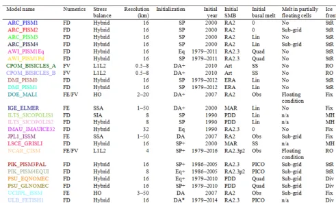
Hélène Seroussi1, Sophie Nowicki2, Erika Simon2, Ayako Abe-Ouchi3, Torsten Albrecht4, Julien Brondex5, Stephen Cornford6, Christophe Dumas7, Fabien Gillet-Chaulet5, Heiko Goelzer8,9, Nicholas R. Golledge10, Jonathan M. Gregory11, Ralf Greve12, Matthew J. Hoffman13, Angelika Humbert14,15, Philippe Huybrechts16, Thomas Kleiner14, Eric Larour1, Gunter Leguy17, William H. Lipscomb17, Daniel Lowry10, Matthias Mengel4, Mathieu Morlighem18, Frank Pattyn9, Anthony J. Payne19, David Pollard20, Stephen F. Price13, Aurélien Quiquet7, Thomas J. Reerink8,21, Ronja Reese4, Christian B. Rodehacke22,14, Nicole-Jeanne Schlegel1, Andrew Shepherd23, Sainan Sun9, Johannes Sutter14,26, Jonas Van Breedam16, Roderik S. W. van de Wal8,24, Ricarda Winkelmann4,25, and Tong Zhang13
1Jet Propulsion Laboratory, California Institute of Technology, Pasadena, CA, USA 2NASA Goddard Space Flight Center, Greenbelt, MD, USA
3University of Tokyo, Tokyo, Japan
4Potsdam Institute for Climate Impact Research (PIK), Member of the Leibniz Association, Potsdam, Germany 5Univ. Grenoble Alpes, CNRS, IRD, Grenoble INP, IGE, 38000 Grenoble, France
6Swansea University, Swansea, UK
7Laboratoire des Sciences du Climat et de l’Environnement, LSCE/IPSL, CEA-CNRS-UVSQ, Université Paris-Saclay, 91191 Gif-sur-Yvette, France
8Institute for Marine and Atmospheric research Utrecht, Utrecht University, Utrecht, the Netherlands 9Laboratoire de Glaciologie, Université libre de Bruxelles, Brussels, Belgium
10Antarctic Research Centre, Victoria University of Wellington, Wellington, New Zealand 11National Center for Atmospheric Science, University of Reading, Reading, UK
12Institute of Low Temperature Science, Hokkaido University, Sapporo, Japan
13Fluid Dynamics and Solid Mechanics Group, Los Alamos National Laboratory, Los Alamos, NM 87545, USA 14Alfred Wegener Institute Helmholtz Centre for Polar and Marine Research, Bremerhaven, Germany
15Department of Geoscience, University of Bremen, Bremen, Germany
16Earth System Science & Departement Geografie, Vrije Universiteit Brussel, Brussels, Belgium
17Climate and Global Dynamics Laboratory, National Center for Atmospheric Research, Boulder, CO, USA 18Department of Earth System Science, University of California Irvine, Irvine, CA, USA
19University of Bristol, Bristol, UK
20Earth and Environmental Systems Institute, Pennsylvania State University, University Park, PA, USA 21Royal Netherlands Meteorological Institute (KNMI), De Bilt, the Netherlands
22Danish Meteorological Institute, Arctic and Climate, Copenhagen, Denmark 23University of Leeds, Leeds, UK
24Geosciences, Physical Geography, Utrecht University, Utrecht, the Netherlands 25University of Potsdam, Institute of Physics and Astronomy, Potsdam, Germany
26Climate and Environmental Physics, Physics Institute, and Oeschger Centre for Climate Change Research, University of Bern, Bern, Switzerland
Correspondence:Hélène Seroussi ([email protected]) Received: 8 December 2018 – Discussion started: 17 January 2019
ice sheets. Following initMIP-Greenland, initMIP-Antarctica has been designed to explore uncertainties associated with model initialization and spin-up and to evaluate the impact of changes in external forcings. Starting from the state of the Antarctic ice sheet at the end of the initialization procedure, three forward experiments are each run for 100 years: a con-trol run, a run with a surface mass balance anomaly, and a run with a basal melting anomaly beneath floating ice. This study presents the results of initMIP-Antarctica from 25 sim-ulations performed by 16 international modeling groups. The submitted results use different initial conditions and initial-ization methods, as well as ice flow model parameters and reference external forcings. We find a good agreement among model responses to the surface mass balance anomaly but large variations in responses to the basal melting anomaly. These variations can be attributed to differences in the extent of ice shelves and their upstream tributaries, the numerical treatment of grounding line, and the initial ocean conditions applied, suggesting that ongoing efforts to better represent ice shelves in continental-scale models should continue.
1 Introduction
The Antarctic ice sheet is the largest reservoir of freshwater on Earth and contains enough ice to raise global mean sea level by 58.3 m (Fretwell et al., 2013). Reconstructions of past sea-level variations show that the volume of the Antarc-tic ice sheet has varied significantly over time, with for ex-ample an ice loss of up to 15 m sea level equivalent (SLE) at a rate of up to 1 mm yr−1 during the Pliocene, around 5.3– 2.6 million years before present (Miller et al., 2012). Sev-eral regions of the Antarctic ice sheet are currently changing rapidly (Rott et al., 2002; Scambos et al., 2004; De Ange-lis and Skvarca, 2003; Khazendar et al., 2013; Mouginot et al., 2014; Rignot et al., 2014; Christie et al., 2016). These changes have been attributed to changes in ocean circulation (e.g., Thomas et al., 2004; Payne et al., 2004; Jenkins et al., 2010, 2018; Jacobs et al., 2012) and atmospheric conditions (e.g., Doake and Vaughan, 1991; Vaughan and Doake, 1996; Scambos et al., 2000). Understanding how the Antarctic ice
climate scenarios (Bindschadler et al., 2013; Nowicki et al., 2013a, b). These results had a large spread for all scenar-ios, as a consequence of differences in model characteristics and processes included, initialization methods, and the inter-pretation and application of model forcings (Nowicki et al., 2013b).
A limitation of these previous efforts was the use of cli-mate forcing that could be considered as outdated by the time of the experiments. For example, the SeaRISE initiative (Sea level Response to Ice Sheet Evolution; Bindschadler et al., 2013) used results from IPCC-AR4 scenarios, while at the same time IPCC-AR5 climate simulations became available. In order to better coordinate the ice sheet modeling and cli-mate modeling communities, the Ice Sheet Model Intercom-parison Project for CMIP6 (ISMIP6) was designed to be the primary activity within the Coupled Model Intercomparison Project Phase 6 (CMIP6) that focuses on the Greenland and Antarctic ice sheets (Nowicki et al., 2016).
sim-ulated present-day ice state might differ significantly from the current observed state, which can impact the sensitivity to perturbations (Pollard and DeConto, 2012a). The second method reproduces present-day ice sheet geometry and ve-locity well but does not capture past climate evolution and current trends of ice mass, due to inconsistencies between datasets (Seroussi et al., 2011), also impacting the ice sheet response to perturbations. To combine the best of these two approaches, models using long transient spin-ups have inte-grated simple inverse methods to match present ice sheet ge-ometry (Pollard and DeConto, 2012a), while models using data assimilation have run short-term relaxation periods to limit the initial shock caused by inconsistent datasets (Gillet-Chaulet et al., 2012). These additions are widening the spec-trum of initialization methods (see also Goelzer et al., 2018). Since ice sheets have a slow response time, their initial conditions influence their evolution for centuries to millen-nia. Understanding the impact of initialization methods is therefore critical for projections of sea level in the 21st cen-tury and beyond. The initMIP experiments were thus de-signed as the first part of ISMIP6, with the goal of under-standing the effects of initialization procedures on model re-sults under simplified and relatively large climate forcings. This effort is intended to show the impact of model initial conditions on the variations in sea level contribution from Antarctica but not to provide improved estimates of sea level evolution. A previous effort, initMIP-Greenland (Goelzer et al., 2018), showed that the initial ice sheet extent has a large impact on Greenland ice sheet evolution when anomalies in surface mass balance (SMB) are applied. Here, we describe a similar effort for the Antarctic ice sheet, using simple climate anomalies applied to both the SMB and to sub-ice-shelf melt-ing rates. We analyze 25 simulations from 16 international groups in order to determine the most relevant factors and to better understand the spread in projections of 21st century Antarctic ice sheet contributions to sea level.
We first describe the initMIP-Antarctica experimental de-sign in Sect. 2 and the participating models in Sect. 3. In Sect. 4, we analyze simulation results and the spread in model responses, and in Sect. 5 we discuss these results and their implications for improving model initialization and constraining sea-level projections. We conclude with re-marks relevant to future modeling efforts.
2 Experiments and model setup
In this section we describe in detail the initMIP-Antarctica experiments, including model requirements and outputs. Complete documentation can be found on the ISMIP6 wiki page (http://www.climate-cryosphere.org/wiki/index. php?title=InitMIP-Antarctica, last access: 7 May 2019).
2.1 Experiments description
InitMIP-Antarctica consists of an initial state,init, describ-ing the initial state of the Antarctic ice sheet model, fol-lowed by three experiments, each designed for continental-scale Antarctic simulations. Modeling groups are asked to describe the ice sheet geometry and other characteristics at the end of their initialization procedure, which is left to the discretion of each group. The following three experiments are 100-year simulations of the Antarctica ice sheet evolu-tion under different forcing scenarios.
In ctrl, the control run, climate forcing is assumed to be similar to present-day conditions, so atmospheric and oceanic forcings at the end of the init experiment are con-tinued unchanged. The total SMB or basal melt applied to the ice sheet can however change, due to, e.g., variations in ice extent during the ctrl simulation.
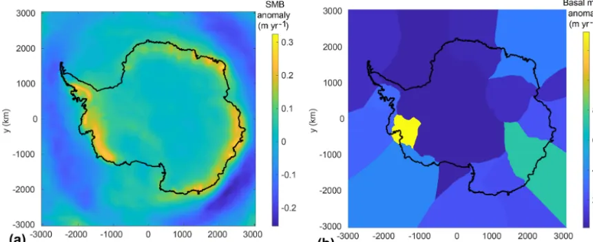
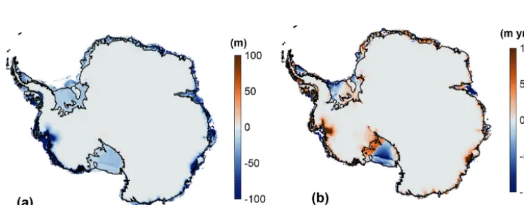
Inasmb, the SMB anomaly experiment, atmospheric forc-ing evolves under a climate-change scenario associated with high greenhouse gas emissions, similar to Representative Concentration Pathway (RCP) 8.5. The prescribed anomaly is the average change in Antarctic SMB for six models: five publicly available CMIP5 RCP8.5 model simulations (Taylor et al., 2012) with large SMB changes between 2006–2010 and 2095–2100, along with one regional model (RACMO2.1; Ligtenberg et al., 2013). As RACMO2.1 re-sults for RCP8.5 were not available when the anomaly field was prepared, we used results for the A1B scenario, with SMB adjusted linearly to reflect the additional radiative forc-ing (an increase of 8.5 W m−2by 2100 in RCP8.5, compared to 6 W m−2in A1B). The RCP8.5 scenario increases precipi-tation by up to 50 % over the Antarctic ice sheet for some cli-mate models (Ligtenberg et al., 2013; Palerme et al., 2016). SMB anomalies are mostly positive over the ice sheet, with a few regions seeing a negative anomaly due to increased sur-face runoff (Fig. 1a). This anomaly is applied over the entire ice sheet.
and [t] the floor function at timet.
These forcings should not be viewed as projections of cli-mate forcing over the coming century, but rather they rep-resent simple perturbations with relatively large changes for the purpose of assessing impacts on Antarctic ice sheet evo-lution.
2.2 Model setup
Ice sheet models are free to use whatever initialization proce-dure is deemed appropriate, given model characteristics and requirements. Submitted simulations rely on long paleocli-mate spin-ups, steady states, data assimilation, or a combi-nation of these methods. There is no constraint or suggestion on forcing datasets (including SMB and sub-shelf melt rates) or on specific physical processes and parameterizations (e.g., basal sliding laws, ice rheology, and stress balance approxi-mation). The initialization time varies among models but is near the beginning of the 21st century.
Previous multi-model ice sheet studies (Bindschadler et al., 2013; Nowicki et al., 2013a, b) showed the difficulty of separating the effects of initial conditions, physical pro-cesses, and external forcings. In order to better analyze the links between initial conditions and external forcings, we im-pose several modeling constraints. Models are required to model floating ice shelves and grounding line dynamics as changes in ice shelves significantly impacted the evolution of West Antarctica in the past decades. The exact procedure to simulate these processes, however, is left at the discre-tion of the modeling groups. Ice sheet models should apply the provided SMB anomalies without adjusting for geomet-ric changes in forward experiments (i.e., surface-elevation feedback). Similarly, they should apply the basal melt rate anomaly under floating ice as it evolves over time. Finally, bedrock elevation adjustment, ice shelf hydrofracturing, and ice cliff failure should not be included, while the ice front evolution is left at the discretion of the modeling groups. 2.3 Model outputs
Modeling groups were requested to report simulation results using a standard output format. Table A1 lists the required outputs, including both scalar and 2-D variables. Scalar
vari-are defined on a polar stereographic projection with standard parallel 71◦S and central meridian 0◦E. Modelers are free to use one of the six prescribed grids with the resolution clos-est to their native resolution. All outputs are then regridded using a conservative interpolation scheme (Jones, 1999) onto an 8 km grid that is used for the analysis. The output grids are identical to the grids used to provide the SMB and basal melt anomalies.
3 Participating models
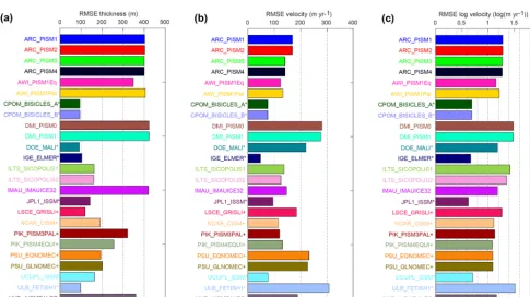
Sixteen modeling centers participated in the initMIP-Antarctica effort and submitted 25 simulations; each model performed the whole suite of experiments. The list of model-ing centers is shown in Table 1. Table 2 lists the main charac-teristics of each simulation, including the stress balance ap-proximation, grid resolution, initialization procedure, initial year, and external forcing. More details on individual models and initialization procedures can be found in Appendix B.
The majority of models use the finite-difference method, with two models based on finite volumes, two based on the finite-element method, and two based on a combination of finite element and finite volume. Two simulations use the Shallow Shelf Approximation (SSA; MacAyeal, 1989), three use L1L2 (i.e. depth-integrated higher-order) approximations (Hindmarsh, 2004), and two use a 3-D higher-order approx-imation (Pattyn, 2003). The other models use a combination of the Shallow Ice Approximation (SIA; Hutter, 1983) and SSA, either combining SIA for the grounded ice with SSA for the floating ice or using SSA as a sliding law and SIA for the internal deformation (Bueler and Brown, 2009). The grid resolution ranges from 4 to 32 km for models based on fixed regular grids, while models using adaptive grid refine-ment are able to use resolutions as low as 0.5 km in ground-ing zones.
Figure 1. (a) Surface mass balance anomaly (m yr−1) for the asmb experiment and(b)basal melt rate anomaly (m yr−1) for the abmb experiment. Black contours show the current Antarctic ice extent.
described in Pollard and DeConto (2012a). Four models are based on a steady-state equilibrium in which the model is run for an extended period of time, until the ice sheet becomes close to a steady-state equilibrium, with two models also in-cluding present-day geometry as a target (Pollard and De-Conto, 2012a). The remaining seven initializations are based on data assimilation, with three models also including a short relaxation period after the data assimilation to limit the im-pact of inconsistent datasets (Seroussi et al., 2011; Gillet-Chaulet et al., 2012).
For the external SMB forcing, models use output from RACMO2 (Lenaerts et al., 2012), RACMO2.3 (van Wessem et al., 2014), RACMO2.3p2 (van Wessem et al., 2018), MAR (Agosta et al., 2019), ERA Interim (Dee et al., 2011), or Arthern et al. (2006). Five simulations use a positive degree-day scheme (PDD; Reeh, 1991). These choices generate rel-atively similar initial SMB (see Sect. 4). For sub-shelf melt-ing, three simulations do not apply any melt rate. Four oth-ers apply values estimated from remote sensing, extrapolated to regions that unground during the simulation. Most mod-els apply a parameterization that depends linearly (Martin et al., 2011; eight simulations) or quadratically (DeConto and Pollard, 2016; four simulations) on the ocean thermal forc-ing. Three simulations adjust the melt rate using an observed thickness target, and the remaining three simulations use the new Potsdam Ice-shelf Cavity model (PICO) parameteriza-tion (Reese et al., 2018).
Most models include a moving ice front, but five simula-tions have a fixed ice front. Ice front migration is primarily based on strain rate in most cases (Levermann et al., 2012; 10 simulations). Some models use ice flux divergence and accumulated damage at the ice front (Pollard et al., 2015; three simulations), and some have ice-front retreat based on a threshold ice thickness (four simulations), while the others
have retreat only where the ice melts completely (three sim-ulations).
4 Results
4.1 init experiment
Each model reports initial ice sheet conditions at the end of the initialization procedure (init). The total ice-covered area varies between 1.35×10⁷ and 1.50×10⁷km2, a range of only 10.5 % among models. The ice shelf extent, on the other hand, varies significantly among models, from 0.92×10⁶to 2.51×10⁶km2, a range of 6.4 % to 16.7 % of the total ice-covered area. Figure 2 summarizes the initial extent of all models. Some models have ice shelves hundreds of kilome-ters upstream or downstream of their current observed loca-tion. Although models generally agree on the location of the three largest ice shelves (Ross, Ronne–Filchner, and Amery), the location and extent of smaller shelves vary widely, in-cluding in the Amundsen and Bellingshausen Sea sectors. The initial ice mass above floatation varies from 1.79×10⁷ to 2.47×10⁷Gt (between 49.4 and 68.1 m of SLE), while the total ice mass varies from 2.11×10⁷to 2.56×10⁷Gt, in part because of the large discrepancy in ice shelf extent. Table C1 details the main scalar variables in init for all simulations.
be-Tong Zhang Stephen Price
Julien Brondex Fabien Gillet-Chaulet
IGE Elmer/Ice Institut des Géosciences de l’Environnement, France
Ralf Greve ILTS SICOPOLIS Institute of Low Temperature Science,
Hokkaido University, Sapporo, Japan
Heiko Goelzer Thomas Reerink Roderik van de Wal
IMAU IMAUICE Institute for Marine and Atmospheric Research,
Utrecht, the Netherlands
Nicole Schlegel Hélène Seroussi
JPL ISSM Jet Propulsion Laboratory, California Institute of Technology,
Pasadena, USA
Christophe Dumas Aurélien Quiquet
LSCE Grisli Laboratoire des Sciences du Climat et de l’Environnement,
Université Paris-Saclay, France
Gunter Leguy William Lipscomb
NCAR CISM National Center for Atmospheric Research, Boulder, CO, USA
Torsten Albrecht Matthias Mengel Ronja Reese Ricarda Winkelmann
PIK PISM Potsdam Institute for Climate Impact Research, Germany
David Pollard PSU PSU Earth and Environmental Systems Institute, Pennsylvania
State University, University Park, PA, USA
Mathieu Morlighem Helene Seroussi
UCIJPL ISSM University of California, Irvine, USA
Jet Propulsion Laboratory, California Institute of Technology, Pasadena, USA
Frank Pattyn Sainan Sun
ULB f.ETISh Université libre de Bruxelles, Belgium
Jonas Van Breedam Philippe Huybrechts
VUB AISMPALEO Vrije Universiteit Brussel, Belgium
tween observed (Rignot et al., 2011a) and modeled surface velocity (Fig. 3b) also has a large spread among models, varying from 47.5 to 308 m yr−1. These values are signifi-cantly affected by the inclusion of observed surface veloc-ities during the initialization procedure: the RMSE in sur-face speed varies from 47.5 to 94.5 m yr−1 for models in-cluding data assimilation of surface velocities and from 116 to 308 m yr−1 for the other models. Most of these errors
Table 2.List of initMIP-Antarctica simulations and main model characteristics. Numerics rely on the finite-difference (FD), finite-element (FE), or finite-volume (FV) method. Initialization methods are as follows: spin-up (SP), spin-up with target values for the ice thickness (SP+; see Pollard and DeConto, 2012a), data assimilation (DA), data assimilation with short relaxation (DA+), data assimilation of ice geometry (DA∗), equilibrium state (Eq), and equilibrium state with target values for the ice thickness (Eq+). Initial SMB is derived from the following: RACMO2 (RA2; Lenaerts et al., 2012), RACMO2.3 (RA2.3; van Wessem et al., 2014), RACMO2.3p2 (RA2.3p2; van Wessem et al., 2018), MAR (Agosta et al., 2019), ERA Interim (ERA; Dee et al., 2011), Arthern et al. (2006) (Art), and positive degree-day schemes (PDD; Reeh, 1991). Basal melt rates are based on zero melting (0), linear function of thermal forcing (Lin; Martin et al., 2011), quadratic function of thermal forcing (Quad; DeConto and Pollard, 2016), melt rates estimated from observations (Obs; Rignot et al., 2013; Depoorter et al., 2013), ice shelf thickness target (SS), ice shelf thickness target with no refreezing (SS∗), and the PICO parameterization (Reese et al., 2018). Models that have partially floating cells at the grounding line apply melting using a sub-grid scheme (Sub-grid), a floatation condition to assess if melt should be applied over the entire cell or not (Floating condition), or no melt at all (No) in their partially floating cells. Ice front migration schemes are primarily based on strain rate (StR; Levermann et al., 2012), retreat only (RO), fixed front (Fix), minimum thickness height (MH), and divergence and accumulated damage (Div; Pollard et al., 2015). The DMI_PISM1 and DMI_PISM0 differ by the basal melt applied under the floating ice, with a basal melt reduced by an order of magnitude in DMI_PISM1 compared to DMI_PISM0. Further details on all the models are given in Appendix B.
n/a: not applicable.
velocity is small compared to the discrepancies between ob-servations and models, so the exact year used for the initial state has a limited impact on the RMSE calculated.
Area-integrated external forcings (SMB and basal melt) also differ substantially among the models (see Table C1 in the Appendix C). The total initial SMB varies from 2015 to 3430 Gt yr−1, depending on the origin of the SMB forc-ing (see Table 2) and the extent of the ice-covered areas. The total initial ocean-induced basal melt varies from 0 to 2470 Gt yr−1, with seven models having values of less than 150 Gt yr−1, while remote sensing estimates of total Antarc-tic basal melt are ∼1400 Gt yr−1 (Rignot et al., 2013;
De-poorter et al., 2013). Similar to the SMB forcing, these differ-ences result from the chosen melting parameterization (Ta-ble 2) and the geometry of ice shelves.
4.2 ctrl experiment
Figure 2.Initial extent of ice-covered areas and ice shelves for all participating models. All contributions are regridded onto an 8 km standard grid. Figures indicate how many models include ice(a, b)or floating ice(b)in each grid cell. Black lines show the observed ice extent(a)and ice shelf extent(b)from Bedmap2 (Fretwell et al., 2013).
Figure 3.Root mean square error (RMSE) of modeled initial conditions compared to observations for(a)initial ice thickness (m),(b)initial ice surface velocity (m yr−1) over the ice sheet and ice shelf, and(c)the logarithm of the initial ice surface velocity (log(m yr−1)). Please note that the model–color relationship used in this figure is applied in all subsequent figures. Models that assimilate present-day conditions during their initialization process are denoted with+if they integrate geometry and∗if they integrate velocity and geometry information.
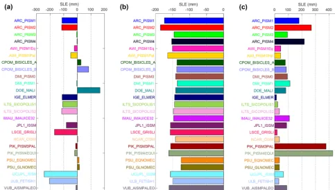
to 167 mm of SLE rise; see Fig. 4a and Table B2), with mass loss in 8 simulations and gain in 17 simulations. This ab-solute change in mass above floatation represents less than 0.42 % of the initial volume in all cases, highlighting the accuracy required to calculate the Antarctic evolution for sea level projections. A spread of results is observed for all initialization methods and model resolutions. Eleven mod-els have an absolute change lower than 20 mm, 10 have
of models in each category is, however, relatively small to draw definitive conclusions.
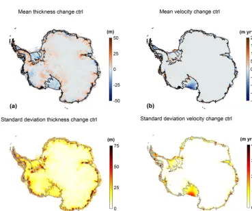
Figure 5 shows the spatial patterns of thickness and depth-average horizontal ice speed for the ctrl experiment. Regrid-ded results on the 8 km standard grid are used to compute modeled mean changes and standard deviation for these two variables. Results are reported only where at least five sim-ulations have ice at a given grid point. Maps of thickness and velocity change during the ctrl experiment show that the signals are larger along the coast than in the interior of the continent and larger in West Antarctica compared to East Antarctica. The ice sheet mean thickness change, averaged over all models, is equal to 1.2 m in 100 years. The standard deviation is calculated for each grid cell of the 8 km standard grid based on the number of models reporting results in each cell and excluding cells where fewer than five models simu-late ice. The standard deviation is much larger than the mean changes in many places, with an average value over the simu-lated area of 14.8 m. Substantial thickening and thinning (es-pecially of ice shelves) compensate for each other, leading to a small spatial average change but large standard devia-tion. Similarly, the spatial average velocity change is small, with a value of −1.9 m yr−1, but the standard deviation is 27.4 m yr−1. Some models have large accelerations in key re-gions, while others have large slowdowns. Regions with the largest spread in model thickness and velocity changes are generally similar.
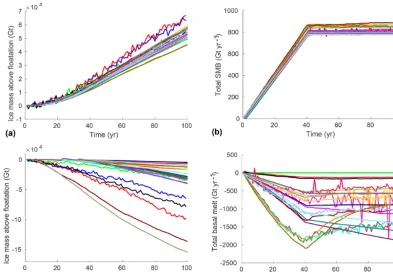
The ice extent is relatively temporally stable in all ctrl sim-ulations, with less than 1.3 % change in the most sensitive simulations. Some simulations, however, have large tempo-ral changes in ice shelf extent, ranging from a reduction of 13 % to an increase of 14 %. The area-integrated SMB varies by up to 6 % for the simulations that experience the largest change in SMB (Fig. 6b). The area-integrated basal melting varies by more than 5 % for 15 models, with a maximum change of 29 %, in response to changes in ice shelf extent and thickness (Fig. 6c).
4.3 asmb experiment
In the asmb experiment, an SMB anomaly (Fig. 1a) is added to the SMB used in the ctrl experiment. This anomaly leads to an increase in ice mass above floatation compared to ctrl, with the mass gain ranging from 4.51×10⁴to 6.72×10⁴Gt (125–186 mm decrease in SLE; see Fig. 4b). The differences among models (Fig. 7a, b) are linked to the extent of the ice-covered areas, as well as ice shelf extent. For most models there is a small increase in grounded area, as some floating areas near grounding lines thicken and reground due to the positive SMB anomaly.
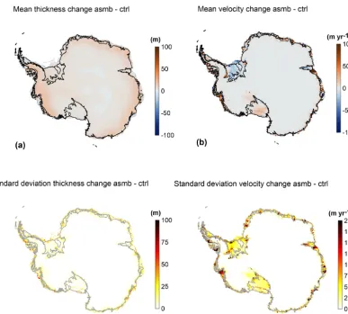
Figure 8 shows the mean and standard deviation of the im-pact of this SMB anomaly on the ice thickness and depth-averaged horizontal velocity. Figure 8 is similar to Fig. 5 but for the difference between the end of the asmb experiment and the end of the ctrl experiment. As expected from the
SMB anomaly spatial pattern (Fig. 1a), there is a thickening of 3.6 m on average over Antarctica, with the largest changes happening along the West Antarctic coasts and the Antarc-tic Peninsula (Fig. 8a). The standard deviation map (Fig. 8c) shows that model differences are again concentrated along the West Antarctica coast and on the Antarctic Peninsula. The average standard deviation over the continent is 5.2 m for this anomaly. The SMB anomaly has a small impact on ice dynamics, as shown in Fig. 8b, with a spatial average speed increase of 1.5 m yr−1 over 100 years and a standard deviation of 17.6 m yr−1. Regions where models disagree are similar to those for the ctrl experiment. Figure 9a compares for each model the difference in mass between the end of the asmb experiment and the end of the ctrl experiment with the cumulative SMB anomaly of the asmb experiment inte-grated over the entire ice sheet. It confirms that the additional SMB is the primary cause of mass change: the SMB anomaly explains between 97 % and 130 % of the total mass change. The difference between the cumulative SMB anomaly and the change in mass is caused by thicker and faster ice (see Fig. 8) that increases the calving flux, as well as feedbacks on ice shelf basal melt.
4.4 abmb experiment
In the abmb experiment, an anomaly is applied to the basal melting rate of floating ice shelves, in addition to the basal melting used in the ctrl experiment. The basal melt anomaly is uniform within each region (see Fig. 1b) and largest in the Amundsen Sea, where an additional ocean-induced melt of 13.2 m yr−1is applied. This additional melting leads to a thinning of ice shelves, a reduction of the buttressing they provide to grounded ice, an acceleration of the ice streams feeding the shelves, and a retreat of grounding lines. How-ever, unlike what is observed for the asmb experiment, the abmb response varies significantly among models.
Differences can be attributed in part to different treatments of basal melt in model cells near the grounding line. Some models have no melting in partially floating cells, others ap-ply melt in partially floating cells based on the fraction of floating area, and two models apply melt over the entire cell if it satisfies a floatation criterion (see Table 2). The spread in ice mass loss above floatation compared to the end of the ctrl experiment varies by 2 orders of magnitude, from 4.7×10³ to 1.5×10⁵Gt (or 13–427 mm of SLE; see Fig. 4c and Ta-ble B2 in Appendix B), even though the additional melt is applied only to floating ice and therefore does not contribute directly to sea level rise. The grounded area is reduced for all the models (between 0.10 % and 1.7 % reduction) as ground-ing lines retreat. The change in ice shelf extent varies from a reduction of 25 % to an increase of 12 %, as some ice shelves calve during this experiment, depending on the choice made for ice front evolution (see Table 2).
Figure 4.Antarctic contribution to sea level (mm of sea level equivalent).(a)ctrl experiment,(b)difference between asmb and ctrl experi-ments, and(c)difference between abmb and ctrl experiments. Negative values of SLE represent a growing ice sheet.
changes are concentrated on the ice shelves and near ground-ing lines. Ice thinnground-ing is 10.7 m on average, and the standard deviation is 12.4 m. The dynamic impact of such variations is not limited to the ice shelves but propagates upstream of the grounding line, especially in the Amundsen Sea Basin, where the largest anomalies are applied. The Ross and Filchner– Ronne ice shelves have acceleration near the grounding line but also a slowdown near the ice front. The modeled mean velocity change over the ice sheet is a small slowdown of 3.3 m yr−1; this signal is small compared to the standard de-viation of 29.6 m yr−1. Regions where models show a large spread of thickness and velocity changes are different from the ctrl and asmb simulations. Large deviations among mod-els extend upstream from the present-day grounding lines and over the ice streams feeding the ice shelves, reflecting different model responses to this oceanic forcing. Figure 9b compares for each model the difference in mass between the end of the abmb experiment and the end of the ctrl experi-ment, with the cumulative basal melt anomaly of the abmb experiment integrated over the entire ice sheet. It shows that the additional basal melt only accounts for a fraction of the mass change: the basal melt anomaly explains between 5 % and 125 % of the total mass change. The difference between the cumulative basal melt anomaly and the change in mass is mainly caused by thinner and slower ice shelves (see Fig. 10) that reduce the calving flux.
5 Discussion
The initMIP-Antarctica experiments are designed to analyze the impact of ice sheet model initial conditions on the evolu-tion of the Antarctic ice sheet and its response to simple cli-mate forcings. For this exercise, 16 groups submitted 25 sim-ulations, more than 4 times the number of Antarctic simu-lations submitted for the SeaRISE project (Bindschadler et al., 2013), highlighting the importance and the fast evolution of this research field (Pattyn et al., 2017). The simulations represent a large diversity of initialization methods, forcing datasets, and model parameters, and the results show a large spread in the mass balance and dynamic evolution of this ice sheet in century-scale simulations.
The initial ice volume above floatation varies from 1.8 to 2.5×10⁷Gt, or almost 32 %, which is much larger than the spread of about 8 % in SeaRISE (Nowicki et al., 2013b). This is not surprising given the larger number of model contri-butions. On the other hand, the largest drifts in the ctrl ex-periment are reduced compared to the SeaRISE project. For initMIP-Antarctica, the ctrl sea level contribution varies be-tween−243 and +167 mm of sea level equivalent for the 25 simulations of ISMIP6, while its evolution varied between
Figure 5.Mean(a, b)and standard deviation(c, d)of the change in ice thickness (aandc, in m) and depth-averaged horizontal velocity (b andd, in m yr−1) between the beginning and end of the ctrl experiment. Black(a, c)or grey(b, d)lines show the observed current ice front and grounding line positions.
Figure 6.Evolution of Antarctic ice sheet mass above floatation and external forcings in the ctrl experiment.(a)Total mass of ice above floatation (Gt),(b)total SMB applied at the ice surface (Gt yr−1), and(c)total basal melting rate (Gt yr−1).
two of them experienced in SeaRISE has been reduced in the initMIP-Antarctica ctrl experiment.
The asmb and abmb experiments are designed to analyze the ice sheet response to simple anomalies in SMB and basal melting under the ice shelves. Unlike initMIP-Greenland, where Goelzer et al. (2018) observed a large spread of 118 % in the responses in the asmb experiment, the response to the SMB anomaly in initMIP-Antarctica is similar among all the models, with a 39 % variation in the response to this anomaly between the models. The differences can be attributed to the larger spread in initial ice sheet extent and the pattern of the
SMB anomaly in initMIP-Greenland. In Greenland, large ab-lation rates are applied at the ice sheet periphery, leading to significant ice loss for the models with the largest initial ex-tents (Goelzer et al., 2018). The Antarctic SMB anomaly has less spatial variability, and the initial extent of the ice sheet is closer for the different simulations, which leads to more consistent responses to this perturbation.
fac-Figure 7.Evolution of the Antarctic ice sheet and external forcings in the asmb (aandb) and abmb (candd) experiments compared to the ctrl experiment. Total amount of ice above floatation for asmb minus ctrl(a)and abmb minus ctrl(c)(in Gt). Evolution of SMB applied at the ice surface for asmb minus ctrl (b, in Gt yr−1) and total basal melting applied in abmb minus ctrl (d, in Gt yr−1).
tors explain the wide range of abmb responses. First, mod-els vary in their treatment of basal melting near the ground-ing line. Elements and grid cells crossed by the groundground-ing line are considered partially floating. Some models have no melting in partially floating cells, others apply melt in par-tially floating cells based on the fraction of floating area, and two models apply melt over the entire cell if it satisfies a floatation criterion (see Table 2). These different treatments can have a significant impact on grounding line evolution, as highlighted by previous studies (Arthern and Williams, 2017; Seroussi and Morlighem, 2018). This is especially important for continental-scale simulations that have a resolution vary-ing between several kilometers and several tens of kilome-ters, as is the case in initMIP-Antarctica. The four largest sea level contributions in the abmb experiment (> 200 mm) come from four models that apply sub-grid melt in par-tially floating cells and have a resolution of 8 km or coarser (see Tables 2 and B2). Additionally, two of these models were run without (ARC_PISM1 and ARC_PISM3) and with (ARC_PISM2 and ARC_PISM4) a sub-grid melt scheme in partially floating cells (see Table 2), which resulted in an ad-ditional sea level rise of 90 and 124 mm when the sub-grid melt scheme was used.
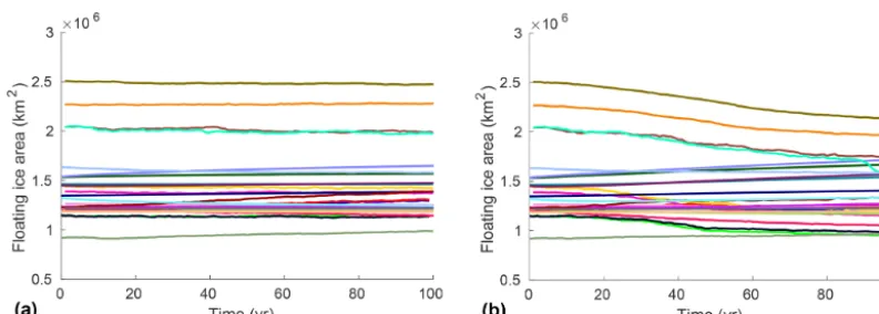
Second, the total ice shelf extent varies by more than 100 % among the different models, and their extent within different basins also varies significantly (see Fig. 2 and
Ta-ble B1). As the basal melting anomaly is applied only un-der floating ice, the spatial extent and amount of the applied anomaly therefore vary significantly from one model to the next. Ice shelf extent also varies during the ctrl and abmb experiments, so that the applied melt anomaly evolves differ-ently between the simulations. As shown in Fig. 11, floating ice areas stay relatively constant in some models, increase because of grounding line retreat in others, and decrease as ice shelves thin significantly and calve in the remaining ones. Third, while the SMB applied in init and ctrl is relatively similar among the different models, the basal melting varies from zero melt to 2140 Gt yr−1. The latter value is about 50 % larger than values derived from remote sensing ob-servations (Rignot et al., 2013; Depoorter et al., 2013) (see Fig. 7). The applied basal melting anomaly therefore repre-sents about half the initial basal melting for some models but a drastic increase for others. The impact on ice shelf thick-ness evolution and dynamic response is therefore very differ-ent, as shown by Fig. 10.
Figure 8.Mean(a, b)and standard deviation(c, d)of the ice thickness (aandc, in m) and depth-averaged horizontal velocity (bandd, in m yr−1) between the end of the asmb experiment and the end of the ctrl experiment. Black(a, b)or grey(c, d)lines show the current observed ice front and grounding line positions.
Figure 10.Mean(a, b)and standard deviation(c, d)of the change in ice thickness (aandc, in m) and depth-averaged horizontal velocity (bandd, in m yr−1) between the end of the abmb experiment and the end of the ctrl experiment. Black(a, b)or grey(c, d)lines show the current observed ice front and grounding line positions.
melting that can drive further thinning and retreat. The effec-tive basal melting anomaly therefore varies between the sim-ulations (see Fig. 7d). These results highlight the need for further modeling studies and observations on basal melting patterns near the grounding line.
One objective of ISMIP6 and initMIP-Antarctica is to gather a large and diverse ice sheet modeling community. To facilitate participation of a large number of models, only two constraints were imposed: (1) the inclusion of both grounded and floating ice and (2) the simulation of dynamic ground-ing line migration. This lack of constraints complicates the analysis of the simulation differences, since model param-eters, input forcing, initialization techniques, and physical processes vary widely among models. Initialization methods that are based on the assimilation of present-day conditions usually have lower RMSE in the initial ice thickness and ve-locity compared to observations (Fig. 3) but larger trends in the ctrl experiment (Fig. 4a), while the opposite is true for models relying on paleoclimate spin-up or a steady-state solution. This is similar to what was previously observed by Nowicki et al. (2013a, b) and Goelzer et al. (2018). As the two approaches are complementary, models are
start-ing to combine them by either followstart-ing data assimilation with short relaxation periods or by assimilating surface ele-vation during transient initialization to have an initial geome-try more consistent with observations (Pollard and DeConto, 2012a). Combining the best of both approaches is an active field of research. Assimilating observations over longer time periods looks like a promising option, despite the technical challenges (Larour et al., 2014; Goldberg et al., 2015).
Figure 11.Evolution of Antarctic ice shelf extent for the(a)ctrl and(b)abmb experiments.
typically is not included in numerical models. Representation of ice shelves varies among models: the ice shelf extent, spa-tial location, and thickness differ significantly between the simulations, resulting in large deviations in ice shelf flow. Another major source of disagreement is the boundary con-dition at the ice–ocean interface, with ocean-induced basal melting applied under the floating ice and its temporal evo-lution based on a wide range of parameterizations. Signifi-cant progress was made over the past decade (Pattyn et al., 2017), but continued improvement of ice shelf representation in continental-scale models should remain a research priority so that ice shelf representation in continental-scale ice sheet models is in better agreement with observations of the cur-rent state of the Antarctic ice sheet.
The results presented in this study rely on simple atmo-spheric and oceanic forcings that are only loosely based on RCP scenarios. Furthermore, many participating models did not use their full capabilities. To reduce model differences, for example, participants were asked to turn off surface-elevation feedback schemes, bedrock adjustment capabili-ties, and ice cliff failure. As a result, the initMIP-Antarctica simulations are not projections of Antarctic evolution over the coming century and should not be compared with pre-vious Antarctic simulations aiming to simulate this evolution (e.g., Ritz et al., 2015; Golledge et al., 2015). The next step of ISMIP6 will be the assessment of Antarctic evolution under different scenarios forced with oceanic and atmospheric con-ditions derived from CMIP climate models; experiments are now being designed. The initMIP-Antarctic simulations do, however, illustrate the spread in ice sheet evolution (hence sea level) that is due to ice sheet model initial state and mod-eling choices (e.g., grounding line numerics, calving laws) and provide insight into uncertainty in simulations of sea level change.
6 Conclusions
The initMIP-Antarctica experiment, part of the Ice Sheet Model Intercomparison Project for CMIP6 (ISMIP6), had
broad participation, with 25 model simulations submitted from 16 groups. Results are improved compared to previ-ous similar exercises of continental-scale modeling of the Antarctic ice sheet, with enhanced representation of present-day conditions and ice mass loss trend. A first experiment performed with a simple surface mass balance anomaly forc-ing produces relatively robust results across the models, while a second experiment with a simple perturbation in basal melting rate under the ice shelves creates very large discrepancies in the ice sheet response. Variations in the rep-resentation of ice shelves (e.g., spatial extent, thickness), ice shelf basal melting, and numerical treatment of grounding lines cause this significant spread of results between the sim-ulations. Including accurate representations of ice shelves that are consistent with observations of the current Antarc-tic ice sheet in continental-scale models should therefore re-main an important research subject in the coming years. All the experiments performed as part of initMIP-Antarctica are based on simplified anomaly forcings. Future projections of the Antarctic ice sheet evolution under different climate sce-narios are currently being designed and will be the subject of future ISMIP6 modeling experiments.
Table A1.Data requests for initMIP-Antarctica. ST: state variable. FX: flux variable. CST: constant.
Variable name Type Standard name Unit
Ice sheet thickness ST land_ice_thickness m
Ice sheet surface elevation ST surface_altitude m
Ice sheet base elevation ST base_altitude m
Bedrock elevation ST bedrock_altitude m
Geothermal heat flux CST upward_geothermal_heat_flux_at_ground_level W m−2
Surface mass balance flux FL land_ice_surface_specific_mass_balance_flux kg m−2s−1
Basal mass balance flux FL land_ice_basal_specific_mass_balance_flux kg m−2s−1
Ice thickness imbalance FL tendency_of_land_ice_thickness m s−1
Surface velocity inxdirection ST land_ice_surface_x_velocity m s−1
Surface velocity inydirection ST land_ice_surface_y_velocity m s−1
Surface velocity inzdirection ST land_ice_surface_upward_velocity m s−1
Basal velocity inxdirection ST land_ice_basal_x_velocity m s−1
Basal velocity inydirection ST land_ice_basal_y_velocity m s−1
Basal velocity inzdirection ST land_ice_basal_upward_velocity m s−1
Mean velocity inxdirection ST land_ice_vertical_mean_x_velocity m s−1
Mean velocity inydirection ST land_ice_vertical_mean_y_velocity m s−1
Ice surface temperature ST temperature_at_ground_level_in_snow_or_firn K
Ice basal temperature ST land_ice_basal_temperature K
Magnitude of basal drag ST magnitude_of_land_ice_basal_drag Pa
Land ice calving flux FL land_ice_specific_mass_flux_due_to_calving kg m−2s−1
Grounding line flux FL land_ice_specific_mass_flux_due_at_grounding_line kg m−2s−1
Land ice area fraction ST land_ice_area_fraction 1
Grounded ice sheet area fraction ST grounded_ice_sheet_area_fraction 1
Floating ice sheet area fraction ST floating_ice_sheet_area_fraction 1
Total ice sheet mass ST land_ice_mass kg
Total ice sheet mass above floatation ST land_ice_mass_not_displacing_sea_water kg
Area covered by grounded ice ST grounded_land_ice_area m2
Area covered by floating ice ST floating_ice_shelf_area m2
Total SMB flux FL tendency_of_land_ice_mass_due_to_surface_mass_balance kg s−1
Total BMB flux FL tendency_of_land_ice_mass_due_to_basal_mass_balance kg s−1
Total calving flux FL tendency_of_land_ice_mass_due_to_calving kg s−1
Appendix B: Model description and initialization Below are descriptions of the ice flow models and the initial-ization procedure performed by the different groups. B1 ARC_PISM
We use the Parallel Ice Sheet Model (PISM) version 0.7.1. PISM is a hybrid ice sheet–ice shelf model that combines shallow approximations of the flow equations that compute gravitational flow and flow by horizontal stretching (Bueler and Brown, 2009). We perform two sets of experiments with different initialization procedures. In the first set (PISM-1,2), the simulations are initialized from the end of a 120 000-year spin-up using paleoclimate forcing, whereas in the second set (PISM-3,4), the simulations are initialized from the end of a 100 000-year spin-up using a constant climate forcing. Both procedures result in a present-day ice sheet configura-tion that is in a thermally and dynamically evolved state, with a “present-day” sea-level equivalent volume of 58.35 and 56.38 m, respectively. The combined stress balance of PISM allows for a treatment of ice sheet flow that is consistent across non-sliding grounded ice to rapidly sliding grounded ice (ice streams) and floating ice (shelves). As with most continental-scale ice sheet models, we use flow enhancement factors for the shallow-ice and shallow-shelf components of the stress regime (3.5 and 0.5, respectively, for PISM-1,2, and 2.8 and 0.5, respectively, for PISM-3,4), which allow us to adjust creep and sliding velocities using simple coeffi-cients. By doing so we are able to optimize simulations such that modeled behavior is consistent with observed behavior. The junction between grounded and floating ice is refined by a sub-grid-scale parameterization (Feldmann et al., 2014) that smooths the basal shear stress field and tracks an inter-polated grounding-line position through time. This allows for much more realistic grounding-line motion, even with rela-tively coarse spatial grids, such as the 16 km grid used in our experiments. We run duplicate experiments with the sub-grid melt turned off (PISM-1,3) or on (PISM-2,4) in order to quantify the effect of this scheme. SMB is calculated us-ing a positive degree-day model that takes as inputs air tem-perature and precipitation from RACMO2.1 (Lenaerts et al., 2012). In previous simulations (e.g., Golledge et al., 2015) we have derived evolving melt beneath ice shelves from the thermodynamic three-equation model of Hellmer and Ol-ber (1989), in which the melt rate is primarily controlled by salinity and temperature gradients across the ice–ocean inter-face. For the simplified experiments presented here, however, we set a spatially uniform melt rate as an initial condition and allow our modeled ice sheet to evolve in response to this. B2 AWI_PISM
The simulations are performed with PISM version 0.7.3. For the 220 ka-long spin-up simulations with paleoclimatic
forcing (PISM1Pal), time slice anomalies for the Last Inter-glacial (LIG) and the Last Glacial Maximum (LGM) from the Earth System Model COSMOS (Pfeiffer and Lohmann, 2016; Zhang et al., 2014) are used in addition to datasets for present-day (PD) Antarctic climate (RACMO2.3, van Wessem et al., 2014; WOA09, Locarnini et al., 2010). Time-dependent and spatially variable climate anomaly fields are interpolated during the PISM run between LIG, LGM, and PD climate time slices with a glacial index method (Sut-ter et al., 2016), where the glacial index is derived from Dome C deuterium depletion (Jouzel et al., 2007). For the SMB, PISM’s positive degree-day (PDD) scheme is used. Relative sea level forcing (Waelbroeck et al., 2002) and bed deformation (Bueler et al., 2007) are applied during the pa-leo spin-up. In addition to the papa-leo spin-up, a 100 ka-long equilibrium-type spin-up (PISM1Eq) with steady present-day climate (ocean and atmosphere) and sea level is car-ried out with isostatic bed deformation. Instead of precipi-tation and 2 m air temperature (PISM1Pal), SMB and skin temperature from RACMO2.3 are directly applied without the PDD scheme. The initial geometry for both spin-ups is Bedmap2 (Fretwell et al., 2013), and the geothermal flux is from Shapiro and Ritzwoller (2004). Basal shelf melt rates are calculated via a quadratic form of the melt rate formula in Beckmann and Goosse (2003) using the extrapolated 3-D ocean temperatures at the depth of the ice shelf base. PISM’s sub-grid grounding line scheme for basal sliding (Feldmann et al., 2014) is used in all simulations.
B3 CPOM_BISICLES
CPOM_BISICLES_A_500m is a block structured adaptive mesh finite-element model based on a vertically integrated stress balance model (Cornford et al., 2013, 2016) and the basal friction physics of Tsai et al. (2015). Here, we make use of the adaptive mesh to maintain a resolution of 8 km in the slow-moving interior, 1 km in ice streams, and 500 m at the grounding line. The initial state is based on ice thick-ness and bedrock elevation from Bedmap2 (Fretwell et al., 2013), modified according to mass conservation close to the grounding line to avoid the large unphysical thickening rates that would otherwise occur, especially in the Amundsen Sea Embayment. Ice temperature is taken from Pattyn (2010) and is held constant in time over the course of the simulations. Effective viscosity ϕ(x, y) and effective drag coefficients β2(x, y)are estimated by minimizing the mismatch between modeled speed the observed speed of Rignot et al. (2011b), following the methods described in Cornford et al. (2015) The background ocean melt rateM0(x, y, t )is defined so that the thinning rate is zero across the ice shelf and varies in time accordingly, so that when a melt rate anomalyMa(x, y, t )is
applied, the ice shelf thinning rate isMa(x, y, t ).
the total precipitation is considered as snow accumulation due to negligible surface melting in Antarctica. Starting from the contemporary ice sheet geometry, both ice internal en-thalpy and temperature evolve for 150 000 years for a fixed ice geometry due to surface and geothermal heat fluxes. Af-terward the model runs freely for 25 000 years, so that the model updates grounded ice margins, grounding lines, and calving fronts continuously. The calving parametrization ex-ploits three sub-schemes for grid points at the ice shelf mar-gins: the eigencalving parameterization (Levermann et al., 2012), which utilizes the stress field divergence with the pro-portionality constant of 5×10¹⁷, the ice shelf margin with a thickness of less than 150 m calve, and ice shelves that ex-tend into the depth ocean calve. Assuming a constant ocean temperature of−1.7◦C and melting factor (Fmelt=0.001), sub-shelf melting follows Eq. (5) in Martin et al. (2011) and occurs only for fully floating grid points, while the grounding line position is determined on a sub-grid space (Feldmann et al., 2014). The basal resistance is described as plastic till for which the yield stress is given by a Mohr–Coulomb formula (Bueler and Brown, 2009; Schoof, 2006). In DMI_PISM1 the basal melting rate of ice shelves is increased by an order of magnitude compared to DMI_PISM0.
B5 DOE_MALI
MPAS-Albany Land Ice (MALI) (Hoffman et al., 2018) uses a three-dimensional, first-order Blatter–Pattyn momentum balance solver solved using finite-element methods. Ice ve-locity is solved on a two-dimensional map plane triangula-tion extruded vertically to form tetrahedra. Mass and tracer transport occurs on the Voronoi dual mesh using a mass-conserving finite-volume first-order upwind scheme. Mesh resolution is 2 km along grounding lines and in all ma-rine regions of West Antarctica and in mama-rine regions of East Antarctica where present-day ice thickness is less than 2500 m to ensure that the grounding line remains in the fine-resolution region, even under full retreat of West Antarctica and large parts of East Antarctica. Mesh resolution coarsens to 20 km in the ice sheet interior and no greater than 6 km in the large ice shelves. The horizontal mesh has 1.6 million cells. The mesh uses 10 vertical layers that are finest near
ice shelf melt rates after grounding line retreat. The SMB is from RACMO2.1 1979–2010 mean (Lenaerts et al., 2012). Maps of SMB and basal mass balance forcing are kept con-stant with time. The ice front position is fixed at the extent of the present-day ice sheet. After initialization, the model is relaxed for 99 years, so that the geometry and grounding lines can adjust.
B6 IGE_Elmer-Ice
B7 ILTS_SICOPOLIS
We use SICOPOLIS version 3.3-dev with either shallow-ice dynamics (ILTS_SICOPOLIS1) or hybrid shallow-shallow-ice– shelfy-stream dynamics (ILTS_SICOPOLIS2; Bernales et al., 2017) for grounded ice and shallow-shelf dynamics for floating ice. Ice thermodynamics is treated with the melting-CTS enthalpy method (ENTM) by Greve and Blatter (2016). The ice surface is assumed to be traction-free. Basal sliding under grounded ice is described by a Weertman-type slid-ing law, with sub-melt slidslid-ing in the form of Sato and Greve (2012). The model is initialized by a paleoclimatic spin-up over 140 000 years, forced by VostokδD converted to1T (Petit et al., 1999), in which the topography is nudged to-wards the present-day topography to enforce a good agree-ment. In the future climate simulations, the ice topography evolves freely. For the last 2000 years of the spin-up and the future climate simulations, a regular (structured) grid with 8 km resolution is used. In the vertical, we use terrain-following coordinates with 81 layers in the ice domain and 41 layers in the thermal lithosphere layer below. The present-day surface temperature is parameterized (Fortuin and Oer-lemans, 1990), the present-day precipitation is by Arthern et al. (2006) and Le Brocq et al. (2010), runoff is mod-eled by the positive degree-day method with the parameters by Sato and Greve (2012), the bed topography is Bedmap2 (Fretwell et al., 2013), and the geothermal heat flux is by Pu-rucker (2012). Present-day ice shelf basal melting is param-eterized as a function of both the depth of ice below mean sea level and ocean temperatures outside the ice shelf fronts at 500 m depth, tuned differently for eight Antarctic sectors (Greve and Galton-Fenzi, 2017).
B8 IMAU_IMAUICE
The finite-difference model (de Boer et al., 2014) uses a com-bination of SIA and SSA solutions, with velocities added over grounded ice to model basal sliding (Bueler and Brown, 2009). The model grid at 32 km horizontal resolution covers the entire Antarctic ice sheet and surrounding ice shelves. The grounded ice margin is freely evolving, while the shelf extends to the grid margin, and a calving front is not ex-plicitly determined. We use the Schoof flux boundary con-dition (Schoof, 2007) at the grounding line with a heuristic rule following Pollard and DeConto (2012b). For the init-MIP experiments, the sea level equation is not solved or cou-pled (de Boer et al., 2014). We run the thermodynamically coupled model with constant present-day boundary condi-tions to determine a thermodynamic steady state. The model is first initialized for 100 kyr using the average 1979–2014 SMB and surface ice temperature from RACMO2.3 (van Wessem et al., 2014) and mapped with OBLIMAP (Reerink et al., 2010, 2016). Bedrock elevation is fixed in time with data taken from the Bedmap2 dataset (Fretwell et al., 2013), and geothermal heat flux data are from Shapiro and
Ritz-woller (2004) and mapped with OBLIMAP (Reerink et al., 2010, 2016). We then run for 30 kyr with constant ice tem-perature from the first run to get to a dynamic steady state, which is our initial condition.
B9 JPL_ISSM
Model setup, as follows, is adapted from Schlegel et al. (2018). The model domain covers the present-day Antarc-tic ice sheet, and its geometry is interpolated from the Bedmap2 dataset (Fretwell et al., 2013), with additional re-finement in the Amundsen Sea sector, Recovery Ice Stream, and Totten Glacier, from Morlighem et al. (2011) and Rignot et al. (2014). The forward simulations rely on a 2-D Shelfy-Stream Approximation (MacAyeal, 1989) for stress balance, with a mesh resolution varying between 1 km at the domain boundary and within the shear margins and 50 km in the in-terior and a resolution of 8 km or finer within the boundary of all initial ice shelves. To estimate land ice viscosity, we compute the ice temperature based on a thermal steady state with 15 vertical layers (Seroussi et al., 2013), using three-dimensional higher-order (Blatter, 1995; Pattyn, 2003) stress balance equations, observations of surface velocities (Rignot et al., 2011b), and basal friction inferred from surface eleva-tions (Morlighem et al., 2010). Thermal boundary condieleva-tions are geothermal heat flux from Maule et al. (2005) and sur-face temperatures from Lenaerts et al. (2012). Steady-state ice temperatures are vertically averaged, used as inputs in the ice flow law, and held constant over time. To infer the un-known basal friction coefficient over grounded ice and the ice viscosity of the floating ice, we use data assimilation (MacAyeal, 1993; Morlighem et al., 2010) to reproduce ob-served surface velocities from Rignot et al. (2011b). Then, we run the model forward for 2 years, allowing the grounding line position and ice geometry to relax (Seroussi et al., 2011; Gillet-Chaulet et al., 2012). The grounding line evolves as-suming hydrostatic equilibrium and following a sub-element grid scheme (SEP2 in Seroussi et al., 2014). The ice front remains fixed in time during all simulations performed, and we impose a minimum ice thickness of 1 m everywhere in the domain. The SMB and the ice shelf basal melt rates used in the control experiment are respectively from the 1979– 2010 mean of RACMO2.1 (Lenaerts et al., 2012) and from the 2004–2013 mean from Schodlok et al. (2016).
B10 LSCE_GRISLI
verti-C-grid in the horizontal plane at 16 km resolution with 21 vertical levels. Atmospheric forcing, namely near-surface air temperature and SMB, is taken from the 1979–2014 clima-tological annual mean computed by the MAR version 3.6.4 regional atmospheric model (Agosta et al., 2019). Initial sub-shelf basal melting rates are the regionally averaged basal melting rates that ensure a minimal ice shelf thickness Eule-rian derivative in a forward experiment with constant climate and fixed grounding line position. The initial ice sheet geom-etry, bedrock and ice thickness, is taken from the Bedmap2 dataset (Fretwell et al., 2013), and the geothermal heat flux is from Shapiro and Ritzwoller (2004).
B11 NCAR_CISM
The Community Ice Sheet Model (CISM; Lipscomb et al., 2019) uses finite-element methods to solve a depth-integrated higher-order approximation (Goldberg, 2011) over the entire Antarctic ice sheet. The model uses a structured rectangular grid with uniform horizontal resolution of 4 km and five vertical σ coordinate levels. The ice sheet is ini-tialized with present-day geometry and an idealized tem-perature profile, then spun up for 30 000 years using 1979– 2016 climatological SMB and surface air temperature from RACMO2.3p2 (van Wessem et al., 2018; Lenaerts et al., 2012). During the spin-up, basal friction parameters (for grounded ice) and sub-shelf melt rates (for floating ice) are adjusted to nudge the ice surface elevation toward present-day observations. This method is a hybrid approach between assimilation and spin-up, similar to that described by Pollard and DeConto (2012a). The geothermal heat flux is taken from Le Brocq et al. (2010). The basal sliding is similar to that of Schoof (2005), combining power-law and Coulomb behav-ior. The grounding line location is determined using hydro-static equilibrium and sub-element parameterization (Glad-stone et al., 2010; Leguy et al., 2014). Basal melt is applied in grid cells that satisfy a floatation condition based on cell thickness and bed elevation; this includes some but not all cells intersected by the grounding line. The calving front is initialized from present-day observations and thereafter is al-lowed to retreat but not advance. See Lipscomb et al. (2019) for more information about the model.
The grounding line position is determined using hydrostatic equilibrium, with sub-grid interpolation of the friction at the grounding line (Feldmann et al., 2014). The calving front po-sition can freely evolve using the eigencalving parameteriza-tion (Levermann et al., 2012). PISM is a thermomechanically coupled (polythermal) model based on the Glen–Paterson– Budd–Lliboutry–Duval flow law (Aschwanden et al., 2012). The three-dimensional enthalpy field can evolve freely for given boundary conditions.
The model is initialized from Bedmap2 geometry (Fretwell et al., 2013), with precipitation from RACMOv2.3 1986–2005 mean (van Wessem et al., 2014) remapped from 27 km resolution and a parameterized ice surface tempera-ture using the positive degree-day scheme (PDD; Huybrechts and de Wolde, 1999, modified by Martin et al., 2011) for PIK_PISM3PAL. In contrast, PIK_PISM4EQUI uses SMB and temperature directly from RACMOv2.3p2 (van Wessem et al., 2018) without PDD. The geothermal heat flux is from Shapiro and Ritzwoller (2004). We use the Potsdam Ice-shelf Cavity model (PICO; Reese et al., 2018) to cal-culate basal melt rate patterns underneath the ice shelves. We use observed ocean temperature and salinity mean val-ues over the period 1975–2012 (Schmidtko et al., 2014) to drive PICO. The Mohr–Coulomb criterion relates the yield stress by parameterizations of till material properties to the effective pressure on the saturated till (Bueler and van Pelt, 2015). Till friction angle is a shear strength parameter for the till material property and is optimized iteratively in the grounded-ice region such that the mismatch of equilibrium and modern surface elevation is minimized. This is analo-gous to the friction-coefficient optimization in Pollard and DeConto (2012a).
B13 PSU_PSUICE
im-posed as a condition on ice velocity across the grounding line. The model includes standard equations for the evo-lution of ice thickness and internal ice temperatures with 10 unevenly spaced vertical layers. Bedrock deformation un-der the ice load is modeled as an elastic lithospheric plate above local isostatic relaxation (ELRA). Basal sliding fol-lows a Weertman-type power law, occurring only where the bed is close to the melt point. Basal sliding coefficients are determined using an inverse method (Pollard and DeConto, 2012a), iteratively matching ice surface elevations to mod-ern observations. Atmospheric temperatures and precipita-tion are obtained from the ALBMAP climatology (Le Brocq et al., 2010), with an imposed sinusoidal cycle for monthly air temperatures, interpolated to the ice sheet grid for SMB calculations. Oceanic melting at the base of ice shelves de-pends on the squared difference between nearby 400 m depth climatological ocean temperature (Levitus, 2012) and the melt point at the bottom of the ice. “Standard” calving of ice shelves is included. InitMIP experiments are run without recently proposed mechanisms of hydrofracturing by surface meltwater and structural failure of large ice cliffs (Pollard et al., 2015; DeConto and Pollard, 2016). The model grid size is 16 km, and two types of initialization are used: (i) spun up to modern equilibrium (for 60 kyr) with constant invariant model climate forcing and (ii) run from 40 ka to modern time using paleoclimate forcing, and the model state at the end of that run is used.
B14 UCIJPL_ISSM
We rely on inverse modeling to initialize the model to present-day conditions, following Morlighem et al. (2013). The mesh horizontal resolution varies from 3 km along the coast (in the vicinity of grounding lines and in shear mar-gins) to 30 km inland and is extruded vertically in 10 lay-ers. We use a higher-order stress balance (Pattyn, 2003) and an enthalpy-based thermal model (Aschwanden et al., 2012; Seroussi et al., 2013). We first perform an inversion of ice shelf viscosity and then an inversion of basal drag under grounded ice, assuming a thermomechanical steady state. Our geometry is primarily based on Bedmap-2 (Fretwell et al., 2013), with local improvements based on mass conserva-tion in the Amundsen Sea Embayment, along the coast of Wilkes Land, and on Recovery Ice Stream (Morlighem et al., 2011; Millan et al., 2017). The thermal model is con-strained by surface temperatures from Comiso (2000) and the geothermal heat flux from Shapiro and Ritzwoller (2004), both included in the SeaRISE dataset (Nowicki et al., 2013b). The SMB used in the control experiment is from RACMO2.3 (van Wessem et al., 2014).
B15 ULB_f.ETISh
The f.ETISh (fast Elementary Thermomechanical Ice Sheet) model (Pattyn, 2017) version 1.3 is a vertically integrated
hybrid finite-difference (SSA for basal sliding; SIA for grounded ice deformation) ice sheet/ice shelf model with ver-tically integrated thermomechanical coupling. The transient englacial temperature field is calculated in a 3-D fashion. The marine boundary is represented by a grounding-line flux con-dition according to Schoof (2007), coherent with power-law basal sliding (power-law coefficient of 2). Model initializa-tion is based on an adapted iterative procedure based on Pol-lard and DeConto (2012a) to fit the model as close as possi-ble to present-day observed thickness and flow field (Pattyn, 2017). The model is forced by present-day SMB and temper-ature (van Wessem et al., 2014), based on the output of the regional atmospheric climate model RACMO2 for the period 1979–2011. The PICO model (Reese et al., 2018) was em-ployed to calculate sub-shelf melt rates, based on present-day observed ocean temperature and salinity (Schmidtko et al., 2014) on which the initMIP forcings for the different basins are added. The model is run on a regular grid of 16 km with time steps of 0.05 year.
B16 VUB_AISMPALEO
Appendix C: Modeled initial conditions
Table C1.Simulated Antarctic initial ice-covered extent, ice shelf extent, ice mass, ice mass above floatation, total SMB, and total basal melt.
Model name Ice extent Ice shelf extent Ice mass Ice mass above Surface mass Basal melt
(106km2) (106km2) (107Gt) floatation (107Gt) balance (Gt) (Gt)
ARC_PISM1 13.696 1.2348 2.5289 2.4656 2686 0
ARC_PISM2 13.696 1.2348 2.5289 2.4656 2686 0
ARC_PISM3 13.579 1.1466 2.3302 2.2785 2493 50
ARC_PISM4 13.579 1.1463 2.3302 2.2785 2493 49
AWI_PISM1Eq 14.112 1.3885 2.4482 2.0979 2672 1233
AWI_PISM1Pal 14.669 1.4364 2.5602 2.1544 3061 1581
CPOM_BISICLES_A 13.654 1.5338 2.4118 2.0734 2144 2141
CPOM_BISICLES_B 13.654 1.5338 2.4118 2.0734 2144 2141
DMI_PISM0 14.270 2.0408 2.1068 1.7873 3427 152
DMI_PISM1 14.270 2.0411 2.1068 1.7873 3427 451
DOE_MALI 13.595 1.4623 2.3794 2.0467 2415 562
IGE_ELMER 13.590 1.3456 2.3885 2.0523 2515 784
ILTS_SICOPOLIS1 13.609 1.1942 2.4050 2.0781 2020 456
ILTS_SICOPOLIS2 13.591 1.2643 2.4092 2.0854 2015 508
IMAU_IMAUICE32 14.174 1.2318 2.3535 2.0573 2706 0
JPL1_ISSM 13.905 1.4522 2.4382 2.1074 2337 986
LSCE_GRISLI 13.956 1.1991 2.4504 2.1081 2602 1565
NCAR_CISM 13.500 1.1850 2.3640 2.0422 2469 1125
PIK_PISM3PAL 14.556 1.2273 2.3574 2.0069 3191 583
PIK_PISM4EQUI 14.230 0.9168 2.3993 2.0466 2795 304
PSU_EQNOMEC 15.043 2.2700 2.4962 1.8772 2639 1278
PSU_GLNOMEC 15.003 2.5063 2.4970 1.8888 2679 1417
UCIJPL_ISSM 13.784 1.3217 2.4289 2.1142 2519 683
ULB_FETISH1 13.889 1.6328 2.3972 2.0612 2660 2468
AWI_PISM1Eq −22.1 −172.3 22.7
AWI_PISM1Pal −48.4 −213.0 −4.5
CPOM_BISICLES_A 26.9 −110.4 105.3
CPOM_BISICLES_B 83.3 −54.3 169.1
DMI_PISM0 0.8 −140.1 94.4
DMI_PISM1 −4.1 −140.0 108.8
DOE_MALI 167.3 −26.6 249.9
IGE_ELMER −111.5 −255.6 −98.3
ILTS_SICOPOLIS1 −107.5 −251.8 −84.9 ILTS_SICOPOLIS2 −115.3 −262.7 −80.0
IMAU_IMAUICE32 0.1 −146.7 108.9
JPL1_ISSM −80.7 −236.8 7.4
LSCE_GRISLI −167.6 −324.6 −149.6
NCAR_CISM 4.1 −137.4 39.3
PIK_PISM3PAL −12.2 −167.8 365.7
PIK_PISM4EQUI −19.8 −181.4 407.0
PSU_EQNOMEC 12.7 −112.0 47.5
PSU_GLNOMEC 16.2 −108.9 50.7
UCIJPL_ISSM −243.6 −400.0 −178.5
ULB_FETISH1 −47.4 −209.7 −22.0