https://doi.org/10.5194/se-10-2015-2019
© Author(s) 2019. This work is distributed under the Creative Commons Attribution 4.0 License.
Actors, actions, and uncertainties: optimizing decision-making
based on 3-D structural geological models
Fabian Antonio Stamm1, Miguel de la Varga1,2, and Florian Wellmann1
1Computational Geoscience and Reservoir Engineering (CGRE), RWTH Aachen University, Germany
2Aachen Institute for Advanced Study in Computational Engineering Science (AICES), RWTH Aachen University, Germany Correspondence:Fabian Antonio Stamm ([email protected])
Received: 15 March 2019 – Discussion started: 27 March 2019
Revised: 11 September 2019 – Accepted: 16 September 2019 – Published: 18 November 2019
Abstract. Uncertainties are common in geological models and have a considerable impact on model interpretations and subsequent decision-making. This is of particular signif-icance for high-risk, high-reward sectors. Recent advances allows us to view geological modeling as a statistical prob-lem that we can address with probabilistic methods. Using stochastic simulations and Bayesian inference, uncertainties can be quantified and reduced by incorporating additional ge-ological information. In this work, we propose custom loss functions as a decision-making tool that builds upon such probabilistic approaches.
As an example, we devise a case in which the decision problem is one of estimating the uncertain economic value of a potential fluid reservoir. For subsequent true value esti-mation, we design a case-specific loss function to reflect not only the decision-making environment, but also the prefer-ences of differently risk-inclined decision makers. Based on this function, optimizing for expected loss returns an actor’s best estimate to base decision-making on, given a probability distribution for the uncertain parameter of interest. We apply the customized loss function in the context of a case study featuring a synthetic 3-D structural geological model. A set of probability distributions for the maximum trap volume as the parameter of interest is generated via stochastic simula-tions. These represent different information scenarios to test the loss function approach for decision-making.
Our results show that the optimizing estimators shift ac-cording to the characteristics of the underlying distribution. While overall variation leads to separation, risk-averse and risk-friendly decisions converge in the decision space and de-crease in expected loss given narrower distributions. We thus consider the degree of decision convergence to be a
mea-sure for the state of knowledge and its inherent uncertainty at the moment of decision-making. This decisive uncertainty does not change in alignment with model uncertainty but de-pends on alterations of critical parameters and respective in-terdependencies, in particular relating to seal reliability. Ad-ditionally, actors are affected differently by adding new in-formation to the model, depending on their risk affinity. It is therefore important to identify the model parameters that are most influential for the final decision in order to optimize the decision-making process.
1 Introduction
implicit geological modeling with probabilistic methods, as presented by de la Varga et al. (2019) with the Python library GemPy.
Building on this probabilistic perspective, we propose the use of custom loss functions as a decision-making tool when dealing with uncertain geological models. In many applica-tions, we are interested in some decisive model output value, for example reservoir volume. Given that such a parameter is the result of a deterministic function of uncertain variables in our model, the parameter of interest is likewise uncertain and can be represented by a probability distribution attained from stochastic simulations. A loss function can be applied to such a distribution to return a case-specific best estimate to base decision-making on.
We consider hydrocarbon exploration and production as an exemplary high-risk, high-reward sector, in which good decision-making is crucial. However, the described meth-ods are potentially equally applicable to other types of fluid reservoirs (e.g., groundwater, geothermal, or CO2 seques-tration) and in the raw materials sector. Monte Carlo simu-lation for reservoir estimation and risk assessment has be-come common in this sector and is often used in combina-tion with decision trees (see Murtha, 1997; Mudford, 2000; Wim and Swinkels, 2001; Bratvold and Begg, 2010). How-ever, it seems to us that distributions resulting from proba-bilistic modeling are mostly only considered to attain best estimates in the form of means. The most likely and ex-treme outcomes are identified as percentiles, typically P50 (the median), P10, and P90. We believe that this practice does not harness the full potential of such a probabilistic distribu-tion and that much of the inherent informadistribu-tion is discarded. Contrary to that, customized loss functions, as a Bayesian method, take into account the full probability distribution and enable the inclusion of various conditions in the process of finding an optimal estimate. While used in statistical deci-sion theory and other scientific fields, loss functions have, to the best of our knowledge, found no significant application in the context of structural geological modeling. Thus, we intend to provide a new perspective with our methodology.
To illustrate our approach of using custom loss functions for decision-making, we first illustrate what such customiza-tion might look like step by step: starting off with a standard symmetrical loss function, incorporating scenario-specific conditions and assumptions, and lastly implementing a fac-tor to represent the varying risk affinities of different de-cision makers. As we assume a petroleum exploration and production decision-making scenario, our parameter of in-terest should be one that indicates the economic value of a potential hydrocarbon accumulation. In a larger context, in-cluding various geological and economic factors such as op-erational expenditures, this could be the net present value (NPV) of a project. In preproduction stages, original oil in place (OOIP) is commonly used for early assessments (Dean, 2007; Morton-Thompson and Woods, 1993). Decision mak-ers would want to best estimate the relevant parameter of
interest to derive recoverable reserves, respective economic value, and subsequently allocate development resources ac-cordingly, which includes the possibility of walking away from a prospect. In this case, the decision maker might refer to an individual geological expert, but also to an exploration company as a whole.
Once we have set up a loss function customized to this de-cision problem, we can apply it to probability density func-tions that represent our knowledge about the true value of the parameter of interest. As mentioned above, such distribu-tions can result from geological modeling in a probabilistic context. To illustrate this, we include a synthetic 3-D struc-tural geological model as a case study. In this context, we define the structurally determined maximum trap volumeVt as our parameter of interest and indicator for economic value. We generate different probability distributions via stochastic simulations and based on various information scenarios. It is important to note that these are always based on the same primary input parameters. We attain altered states of infor-mation by updating the reference case (prior) with secondary information. In doing so, we make sure that the resulting dis-tributions and the realizations of loss function applications can be directly compared. These case studies are synthetic and chosen here to exemplify the application of Bayesian de-cision theory and to show how additional information affects the optimality of decisions.
2 Methods
2.1 Bayesian decision theory
We view the statistical analysis of geological models from a probabilistic perspective, which is most importantly charac-terized by its preservation of uncertainty. Its principles have been presented and discussed extensively in the literature (see Jaynes, 2003; Box and Tiao, 2011; Harney, 2013; Gel-man et al., 2014; Davidson-Pilon, 2015). The Bayesian ap-proach is widely seen as intuitive and inherent in the natural human perspective. It regards probability as a measure of be-lief about a true state of nature.
2.1.1 Loss, expected loss, and loss functions
Common point estimates, such as the mean and the median of a distribution, usually come with a measure for their accuracy (Berger, 2013). However, it has been argued by Davidson-Pilon (2015) that using pure accuracy metrics, while this technique is objective, ignores the original intention of con-ducting the statistical inference in cases in which payoffs of decisions are valued more than their accuracies. A more ap-propriate approach can be seen in the use of loss functions (Davidson-Pilon, 2015).
Loss is a statistical measure of how “bad” an estimate of the parameter /t het a is. Estimate-based decisions are also referred to as actionsa. Therefore, we also refer to decision makers as actors. Loss is defined asL(θ, a), soL(θ1, a1)is the actual loss incurred when action a1 is taken, while the true state of nature is θ1 (Berger, 2013). The magnitude of incurred loss related to an estimate is defined by a loss func-tion, which is a function of the estimate and the true value of the parameter (Wald, 1950; Davidson-Pilon, 2015):
L(θ,θ )ˆ =f (θ,θ ).ˆ (1)
So, how “bad” a current estimate is depends on the way a loss function weights accuracy errors and returns respective losses. Two standard loss functions are the absolute-error and the squared-error loss function. Both are objective, symmet-ric, simple to understand, and commonly used.
The presence of uncertainty during decision-making im-plies that the true parameter value is unknown and thus the truly incurred loss L(θ, a)cannot be known at the time of making the decision. The Bayesian perspective considers un-known parameters to be random variables and samples that are drawn from a probability distribution to be possible re-alizations of the unknown parameter; i.e., all possible true values are represented by this distribution.
Under uncertainty, the expected loss of choosing an es-timate θˆ over the true parameter value θ is defined by (Davidson-Pilon, 2015)
l(θ )ˆ =E
θ[L(θ,θ )ˆ ]. (2)
The expectation symbol Eis subscripted withθ, by which it is indicated thatθis the respective unknown variable. This expected losslis also referred to as the Bayes risk of estimate
ˆ
θ(Berger, 2013; Davidson-Pilon, 2015).
By the law of large numbers, the expected loss of θˆ can be approximated by drawing a large sample sizeN from the posterior distribution, applying a loss function L, and aver-aging over the number of samples (Davidson-Pilon, 2015):
1 N
N X
i=1
L(θi,θ )ˆ ≈Eθ[L(θ,θ )ˆ ] =l(θ ).ˆ (3)
Hereby, we can approximate the expected loss l for every possible estimateθˆ(every decision we can make) according
to the loss function in use. Minimization of a loss function re-turns a point estimate known as a Bayes action or a Bayesian estimator, which is the decision with the least expected loss according to the loss function and the decision in which we are interested in this work (Berger, 2013; Moyé, 2006). 2.1.2 Customization of our case-specific loss function Davidson-Pilon (2015) and Hennig and Kutlukaya (2007) have proposed that it might be useful to move on from stan-dard objective loss functions to the design of customized loss functions that specifically reflect an individual’s (i.e., the decision maker’s) objectives and preferences regarding outcomes. Especially as we assign an economic notion to ge-ological models and related estimation problems, we argue that it is necessary to consider the subjective perspectives of involved decision makers, for example exploration and production companies. Consequently, the design of a more specific nonstandard and possibly asymmetric loss function might be required, one that includes subjective aspects and differences in weighting of particular risks, arising from a decision maker’s inherent preferences and the environment in which this actor has to make a decision. In the face of several uncertain parameters, which is a given in complex geological models, a perfect estimate, a perfect decision, is virtually unattainable. However, an attempt can be made to design a custom loss function that returns a Bayesian estima-tor involving the least bad consequences for a decision maker in a specific environment (Davidson-Pilon, 2015; Hennig and Kutlukaya, 2007).
Hennig and Kutlukaya (2007) argue that choosing and de-signing a loss function involves the translation of informal aims and interests into mathematical terms. This process nat-urally implies the integration of subjective elements. Accord-ing to them, this is not necessarily unfavorable or less objec-tive, as it may better reflect an expert’s perspective on the situation.
Standard symmetric loss functions can easily be adapted to be asymmetric, for example by weighting errors to the neg-ative side stronger than those to the positive side. Preference over estimates larger than the true value, i.e., overestimation, is thus incorporated in an uncomplicated way. Much more complicated designs of loss functions are possible, depend-ing on purpose, objective, and application. We will describe potential design options in the following.
unknown true value in the form of over- and underestimation bring about an error and loss accordingly.
It can be assumed that several decision makers in one such environment or sector may have the same general loss func-tion but different affinities concerning risks. This might be based, for example, on different psychological factors or eco-nomic philosophies followed by companies. It might also be based on the budgets and options such actors have available. An intuitive example is the comparison of a small and a large company. A false estimate and wrong decision might have a significantly stronger impact on a company that has a gen-erally lower market share and few projects than on a larger company that might possess higher financial flexibility and for which one project is only one of many development op-tions in a wide portfolio.
In steps I–IV we make assumptions about the significance of such deviations and how they differently contribute to ex-pected losses in the general decision-making environment and introduce the concept of varying risk affinities in the final step V.
– Step I – Choosing a standard loss function as a starting point.In our case, we assume that investments increase linearly with linear growth in the value of the prospect. For this reason, we choose the symmetric absolute-error loss function as a basis for further customization steps:
L(θ,θ )ˆ = |θ− ˆθ|. (4)
– Step II – Simple overestimation.Considering the devel-opment of a hydrocarbon reservoir, it can be assumed that over-investing is worse than under-investing. Over-estimating the size of an accumulation might, for ex-ample, lead to the installation of equipment or facilities that are actually redundant or unnecessary. This would come with additional unrecoverable expenditures. Con-sequences from underestimating (0<θ < θ), however,ˆ may presumably be easier to resolve. Additional equip-ment can often be installed later on. Hence, simple over-estimation (0< θ <θ) is weighted stronger in this lossˆ function by multiplying the error with an overestimation factora:
L(θ,θ )ˆ = |(θ− ˆθ )|a. (5)
– Step III – Critical overestimation. The worst case for any project would be that its development is set into motion expecting a gain only to discover later that the value in the reservoir does not cover the costs of realiz-ing the project, resultrealiz-ing in an overall loss. A petroleum system might also turn out to be a complete failure con-taining no value (Vt=0 in our 3-D case study) at all, al-though the actor’s estimate indicated the opposite. Here, we refer to this as critical overestimation. A positive value is estimated, but the true value is zero or negative
(θ≤0<θ). This is worse than simple overestimation,ˆ whereby both values are positive and a net gain is still achieved, which is only smaller then the best possible gain of expecting the true value. Critical overestimation is included in the loss function by using another weight-ing factorbthat replacesa:
L(θ,θ )ˆ = |(θ− ˆθ )|b. (6)
In other words, with b=2, critical overestimation is twice as bad as simple overestimation.
– Step IV – Critical underestimation.We also derive criti-cal underestimation from the idea of estimating zero (or a negative value) when the true value is actually positive (θˆ≤0< θ). This is assumed to be worse than simple overestimation but clearly better than critical overesti-mation. No already owned resources are wasted, and it is only the potential value that is lost, i.e., opportu-nity costs that arise from completely discarding a prof-itable project. Critical underestimation is weighted us-ing a third factorc:
L(θ,θ )ˆ = |(θ− ˆθ )|c. (7)
– Step V – Including different risk affinities.We now fur-ther adapt the loss function to consider varying risk affinities of different actors. We follow the approach of Davidson-Pilon (2015), who implemented different risk affinities by simply introducing a variable risk factor. Using different values for this factor, we can represent how comfortable an individual is with being wrong and furthermore which “side of wrong” is preferred by that decision maker (Davidson-Pilon, 2015). In our case, bidding lower is considered the cautious, risk-averse op-tion, as smaller losses can be expected from underes-timating. Guessing higher is deemed riskier, as losses from overestimation are greater. However, bidding cor-rectly on a higher value will also return a greater gain. It is assumed that risk-friendly actors care less about crit-ical underestimation; i.e., they would rather develop a project than discard it. In our finalized loss function, we simply include these considerations via a risk affinity factorr, which alters the incurred losses:
L(θ,θ )ˆ =
|θ− ˆθ|r−0.5, for 0<θ < θˆ |θ− ˆθ|a r, for 0< θ <θˆ |θ− ˆθ|b r, forθ≤0<θˆ |θ− ˆθ|c r−0.5, forθˆ≤0< θ ,
witha, b, c, r∈Q. (8)
basically any numerical values but should be chosen in a way that they appropriately represent the framework conditions of the problem. Here, we assume that simple overestimation is 25 % (a=1.25), critical overestimation 100 % (b=2), and critical underestimation 50 % (c=1.5) worse than simple underestimation.
According to Eq. (8), the risk-neutral loss function is re-turned for r=1, as no reweighting takes place. Forr <1, the weight on overestimating (a,b) is reduced and increased for critical underestimation (c), as well as normal underesti-mation. This represents a risk-friendlier actor that is willing to bid on a higher estimate to attain a greater gain. Forr >1, the overestimation weight (a,b) is increased in the loss func-tion, underestimation and critical underestimation weight (c) are decreased, and more risk-averse actors are prompted to bid on lower estimates. Since risk neutrality is expressed by r=1, we consider values 0< r <2 to be the most appropri-ate choices to represent both sides of risk affinity equally.
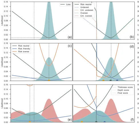
In Fig. 1, we illustrate different aspects and steps of adapt-ing and applyadapt-ing the custom loss function. For these simple examples, we assume that the economic value of our reser-voir is represented by an abstract score parameter. Figure 1a depicts the plotting of the absolute-error loss function (cus-tomization step I) applied to a normal distribution. It can be seen that for this standard symmetrical function, the mini-mal point of expected losses and Bayes action corresponds to the median (and mean for this symmetric distribution). Figure 1b summarizes customization steps II–IV and visual-izes how four different functions for four cases of under- and overestimation are summed up to one combined loss function that comprises all of the assumptions made for the decision-making environment. A jump of expected losses on the nega-tive side of possible estimates can be attributed to the way we defined the function for critical underestimation as dependent on zero.
In Fig. 1c, the risk factor of step V was implemented with-out steps II–IV, i.e., only for the standard absolute-error loss function. It can be seen that risk-averse and risk-friendly de-cision makers are represented by different realizations of ex-pected losses based on one and the same normal distribution: the narrow shape of the risk-friendly function represents im-proved confidence in the decision, while the increased ex-pected loss (Bayes risk) of the minimum indicates that this comes along with the acceptance of a higher risk. Inversely, the flat shape of the risk-averse function can be seen as re-duced confidence in the decision. There is less of a difference in making a different decision than for the risk-friendly ac-tor. At the same time, the expected loss of the minimum, and thus the accepted risk, is lower. However, although they differ in expected losses, both decision makers share the same in-dividual best estimate, since the loss function in itself is still symmetric. This changes in panel (d), in which all customiza-tion steps were applied. Here, the risk factor reweights the influence of the subfunctions shown in panel (b). Under- and overestimation cases are accordingly enhanced or reduced in
impact so that the resulting loss function becomes asymmet-ric and minima are found at different score estimates, given the same underlying information.
In Fig. 1e and f, the functions from panels (c) and (d) are applied on a score distribution resulting from the combina-tion of two other uncertain parameters: reservoir thickness and depth. This can be seen as an extremely simplified 1-D model with only two inputs that define one output as a param-eter of interest, the final score. In this case, thickness is seen as the potential positive value in our reservoir, as it provides space for hydrocarbons to accumulate. Depth is subtracted from this, as it implies a cost of drilling. Thus, the final score is a very essential representation of the economic value given the information available. The respective final distribution is slightly skewed. Figure 1e depicts the respective application of the same functions used in panel (c): symmetric, but in-cluding risk affinity. The overall effects are the same as in panel (c). It can be additionally observed that since the under-lying distribution is now asymmetric, all expected loss min-ima are found on the median estmin-imate, lower than the mean. In panel (f), the complete custom loss function was applied as in panel (d). Based on the uncertain information about the final score, the three differently risk-affine loss functions plot differently, with minima in the negative space, at zero, and in the positive space. This illustrates how the risk-averse de-cision maker tends to expect a possible negative outcome, while the risk-friendly actor bids on a positive value. This could be seen as the decision to abandon versus the decision to invest in a prospect.
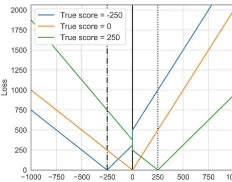
For a better understanding of how our finalized custom loss function determines the incurrence of loss, actual losses for three fixed true values and risk neutrality (r=1) are plot-ted in Fig. 2.
It has to be emphasized that this is just one possible pro-posal for loss function customization. There is not one per-fect design for such a case (Hennig and Kutlukaya, 2007). Slight to strong changes can already be implemented by sim-ply varying the values of the weighting factorsa,b, andc. Fundamentally different loss functions can also be based on a significantly different mathematical structure. As loss func-tions are customized regarding the problem environment and according to the subjective needs and objectives of the de-cision maker, they are mostly defined by the actor express-ing his or her perspective (Davidson-Pilon, 2015; Hennig and Kutlukaya, 2007). Changes in the individual’s perception and attitude might lead to further customization needs at a future point in time, as reported by Hennig and Kutlukaya (2007). 2.2 Case study: synthetic 3-D structural geological
model
Figure 1.Illustration of different steps and aspects of our loss function customization. Functions are applied to an abstract score as the parameter of interest.
encompass numerous uncertain input parameters. As a case study, we now consider a synthetic 3-D structural geological model that is placed in a probabilistic framework.
2.2.1 Computational implementation
Computationally, we implement all of our methods in a Python programming environment, relying in particular on the combination of two open-source libraries: (1) GemPy (version 1.0) for implicit geological modeling and (2) PyMC (version 2.3.6) for conducting probabilistic simulations.
GemPy is able to generate and visualize complex 3-D structural geological models based on a potential-field in-terpolation method originally introduced by Lajaunie et al.
(1997) and further elaborated by Calcagno et al. (2008). GemPy was specifically developed to enable the embedding of geological modeling in probabilistic machine-learning frameworks, in particular by coupling it with PyMC (de la Varga et al., 2019).
ap-Figure 2. Loss based on the risk-neutral custom loss function (Eq. 8) for determined true scores of−250, 0, and 250. This plot is meant to clarify the way real losses are incurred for each esti-mate relative to a given true value. The expected loss, as seen in Fig. 1, is acquired by arithmetically averaging over all deterministic loss realizations based on the score probability distribution by using Eq. (3).
proach by Geweke (1991). Components of a statistical model are represented by deterministic functions and stochastic variables in PyMC (Salvatier et al., 2016). We can thus use the latter to represent uncertain model input parameters and link them to additional data via likelihood functions. Other parameters, such as the value of interest for decision-making, can be determined over deterministic functions as children of parent input parameters.
To visually compare the states of geological unit probabil-ities after conducting stochastic simulations, we consider the normalized frequency of lithologies in every single voxel and visualize the results in probability fields (see Wellmann and Regenauer-Lieb, 2012).
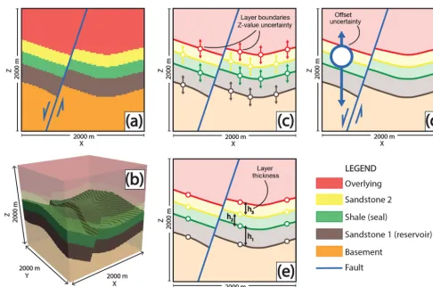
2.2.2 Design of the 3-D structural geological model Our geological example model is designed to represent a potential hydrocarbon trap system. Stratigraphically, it in-cludes one main reservoir unit (sandstone), one main seal unit (shale), an underlying basement, and two overlying for-mations that are assumed to be permeable so that hydrocar-bons could have migrated upwards. Structurally, it is con-structed to feature an anticlinal fold that is displaced by a normal fault. All layers are tilted and dip in the opposite di-rection of the fault plane dip. A potential hydrocarbon trap is thus found in the reservoir rock enclosed by the deformed seal and the normal fault.
Using GemPy, we construct the geological model as fol-lows: in principle, it is defined as a cubic block with an extent of 2000 m in thex,y, andzdirections. The basic input data for the interpolation of the geological features is composed of
Table 1.Input parameter uncertainties defined by distributions with respective meansµ, standard deviationsσ, and shape factorα.
µ σ α
Overlying 0 40 0
Sandstone 2 0 60 0
Seal 0 80 0
Reservoir 0 100 0
Fault offset 0 −150 −2
3-D point coordinates for layer interfaces and fault surfaces, as well as orientation measurements that indicate respective dip directions and angles. From these data, GemPy is able to interpolate surfaces and compute a voxel-based 3-D model (see Fig. 3).
We include uncertainties by assigning them to thez po-sitions of points that mark layer interfaces in the 3-D space. This is achieved via probability distributions (PyMC stochas-tic variables) from which error values are drawn. These are then added to the original input datazvalue. As thezposition is the most sensible parameter for predominantly horizontal layers, we can hereby not only implement uncertainties re-garding layer surface positions in depth, but also layer thick-nesses, geometrical shapes, and degree of fault offset.
Such probability distributions can also be allocated as homogeneous sets to point and feature groups that are to share a common degree of uncertainty (see Table 1). We as-sign the same base uncertainty to groups of points belong-ing to the same layer bottom surface by referrbelong-ing them to one shared distribution each. Assuming an increase in un-certainty with depth, standard deviations for the shared dis-tributions are increased for deeper formations. Furthermore, uncertainty regarding the magnitude of fault offset is incor-porated by adding a skewed normal probability distribution that is shared by all layer interface points in the hanging wall. A left-skewed normal distribution is chosen to reflect the na-ture of throw on a normal fault, in particular the slip motion of the hanging wall block. Skew to the negative side ensures that the offset nature of the normal fault is maintained and inversion to a reverse fault is avoided.
This model was designed for the primary purpose of test-ing our loss function method. All features, uncertainties, and parameter relations were implemented in a way that they re-sult in model variability and complexity that is adequate and significant to the decision problem in this work. The model is not aimed at representing a completely plausible or realistic geological setting.
2.2.3 Vtas the parameter of interest
Figure 3.Design of the 3-D structural geological model. A 2-D cross section through the middle of the model (y=500 m), perpendicular to the normal fault (parallel to thex–zplane), is shown in(a). A 3-D voxel representation of the model, highlighting the reservoir and seal formations, is visualized in(b). In(c)and(d), the inclusion of parameter uncertainties is presented. Colors indicate certain layer bottoms (i.e., boundaries) that are assigned sharedz-positional uncertainties(c). All points in the hanging wall are additionally assigned a fault offset uncertainty(d). Thicknesses of the three middle layers are defined by the distances of boundary points(e)and are thus directly dependent on(c).
calculations, we assume that closed traps are always filled to spill; i.e., we only consider structural features as control-ling mechanisms and disregard other parameters in the OOIP equation (Eq. 9).
We argue thatVtcan be inserted for the hydrocarbon-filled rock volumeA·hin the OOIP equation (Dean, 2007; Morton-Thompson and Woods, 1993):
OOIP=A·h·φ·(1−SW)·1/FvF, (9) where OOIP is returned in cubic meters, Ais the drainage area,h the net pay thickness,φthe porosity, SWthe water saturation, and FvF the formation volume factor that deter-mines the shrinkage of the oil volume brought to the surface. By declaring these connections, we have given our model an economic significance. We can assume that the hydrocar-bon trap volume is directly linked to project development de-cisions; i.e., the investment and allocation of resources is rep-resented by bidding on a volume estimate.
In the course of this work, we developed a set of algo-rithms to enable the automatic recognition and calculation
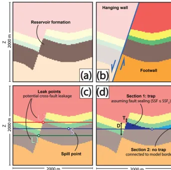
of trap volumes in geological models computed by GemPy. The volume is determined on a voxel-counting basis via four conditions illustrated in Fig. 4 and further explained in Ap-pendix A.
Figure 4.Illustration of the process of trap recognition in 2-D, i.e., the conditions that have to be met by a model voxel to be accepted as belonging to a valid trap. A voxel has to be labeled as part of the target reservoir formation(a)and positioned in the footwall(b). Trap closure is defined by the seal shape and the normal fault(c). Consequently, the maximum trap fill is defined by either the anticlinal spill point (S) or a point of leakage across the fault, depending on juxtapositions with layers underlying (L1) or overlying the seal (L2). The latter is only relevant if the critical shale smear factor is exceeded, as determined overDandT in(d). In this example, assuming sealing of the fault due to clay smearing, the fill horizon is determined by the spill point in(d). Subsequently, only trap section 1 is isolated from the model borders in(d)and can thus be considered a closed trap. Voxels included in this section are counted to calculate the maximum trap volume.
2.2.4 Generating different probability distributions for Vt
The trap volume Vt is a result from GemPy’s implicit geo-logical model computation. It is an output parameter depen-dent on deterministic and stochastic input parameters. When conducting stochastic simulations, input uncertainties will propagate to Vt, which is thereby represented by a respec-tive probability distribution that our custom loss function can be applied to. Using simple Monte Carlo error propagation, with every iteration, we draw sample values for our uncer-tain primary model input parameters defined in Sect. 2.2.2, and thus, with every iteration, we create one possible realiza-tion of our geological model, which in turn comes with one possible outcome forVt. Results from all iterations together approximate the probability distribution forVt according to the input parameters.
Furthermore, we consider the possibility of updating our model by adding additional secondary information via Bayesian inference. We do this by introducing likelihood functions that constrain our primary parameters. We have to note that these inputs remain unchanged; however, their prior probability distributions are revalued given the additional sta-tistical information. We achieve this by conducting Markov chain Monte Carlo (MCMC) simulations. Decision-making is then based on the resulting posterior probability. Using dif-ferent likelihood functions, we can create and generate differ-ent posterior probability distributions forVt, which represent different information scenarios. Since we use Bayesian infer-ence to revalue our original prior inputs, we can compare all outcomes and realizations of our custom loss function.
1. Layer thickness likelihoods.With every model realiza-tion, we extract the z distance between layer bound-ary input points at a centralx–y position (x=1100 m, y=1000 m) in our input interpolation data. Resulting thicknesses can then be passed on to stochastic func-tions in which we define thickness likelihoods via nor-mal distributions.
2. Shale smear factor (SSF) likelihood.SSF values are re-alized over more complex parameter compositions. We base this likelihood on a normal distribution that we link to the geological model output.
The inclusion of these likelihoods is based on purely hypo-thetical assumptions and is intended to provide the opportu-nity to explore the effects that different types and scenarios of additional information might have. While the thickness like-lihood functions are dependent on input parameters directly, the implementation of the SSF likelihood function requires a full computation of the model and extended algorithms of structural analysis.
Although Bayesian inference was utilized in this case study, it served primarily for the generation of these different but comparable distributions on which to base our decision-making, i.e., the application of our custom loss function. For additional information on how implicit geological modeling can be embedded in a Bayesian framework and how this can be used to reduce uncertainty, we refer to the work by Well-mann et al. (2010b), de la Varga and WellWell-mann (2016), de la Varga et al. (2019), and Wellmann et al. (2017).
3 Results
We applied our custom loss function to various different Vt probability distributions resulting from stochastic simu-lations. First, reference results were created using only pri-mary inputs (priors) and simple Monte Carlo error prop-agation (10 000 sampling iterations, Scenario 1). Then we devised several scenarios of additional information and in-cluded these via likelihoods and Bayesian inference. For this, 10 000 MCMC sampling steps were conducted, with an ad-ditional burn-in phase of 1000 iterations. The prior parame-ter uncertainties were chosen to be identical for all simula-tions (see Table 1). Results of convergence diagnostics can be found in Appendix C.
We present the following information scenarios. 1. Prior-onlymodel
2. Introducingseal thickness likelihoods
a. Likely thick seal b. Likely thin seal
3. Introducingreservoir thickness likelihoods
a. Likely thick reservoir
b. Likely thick reservoir and thick seal 4. IntroducingSSF likelihoods
a. SSF likely near its critical value b. Likely reliable SSF and thick seal The implemented likelihoods are listed in Table 2.
For the comparison of results, we consider in particular the following measures: (1) probability field visualization, (2) occurrence of trap control mechanisms, (3) resulting trap volume distributions, and (4) consequent realization of ex-pected losses and related decisions.
3.1 Prior-only model (Scenario 1)
Probability field visualization illustrates well how the prior uncertainty is based on normal distributions (see Fig. B2). Trap control mechanisms are listed in Table B2. For this prior-only scenario, all four relevant mechanisms occur. The dominant factor is the anticlinal spill point with a 51.5 % rate of occurrence. It is followed by cross-fault leakage to the reservoir (25 %) and other permeable formations (12 %). Stratigraphical breaches of the seal were registered to be de-cisive in about 11 % of iterations. In only 0.5 % of iterations, the algorithm failed to recognize a mechanism; i.e., correct model realization failed.
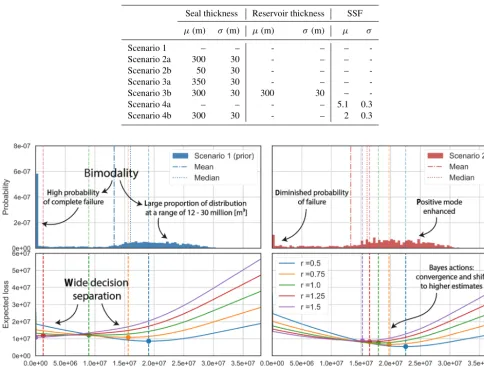
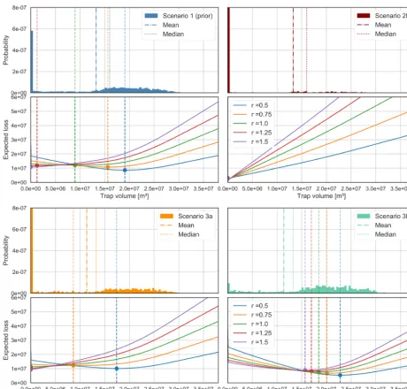
Maximum trap volumes were calculated for each model iteration and plotted as a probability distribution in Fig. 5. In general, a wide range of volumes is possible, from zero to more than 3 million m3. However, we can recognize a bi-modal tendency: low volumes are less probable than signifi-cantly high volumes or complete failure (Vt=0).
Consequently, applying our custom loss function to this distribution resulted in widely separated minimizing estima-tors for the differently risk-inclined acestima-tors (see Fig. 5). Only the risk-friendliest estimates are found within the described highly positive mode of the distribution. Risk-averse individ-uals bid on significantly lower estimates or even zero. The risk-neutral decision is found between the two modes and presents the highest expected loss. Expected losses decrease towards the extreme decisions and closer to the modes. 3.2 Introducing seal thickness likelihoods (Scenarios 2a
and 2b)
We considered two scenarios of thickness likelihoods: the seal being (Scenario 2a) likely very thick or (Scenario 2b) likely very thin (see Table 2).
In Scenario 2a, probability visualization illustrates that the presence of a thick seal is very probable (see Fig. B2). For Scenario 2b, the presence of a reliable seal is questionable.
Table 2.Normal distribution mean (µ) and standard deviations (σ) for the likelihoods implemented in the different scenarios.
Seal thickness Reservoir thickness SSF
µ(m) σ(m) µ(m) σ(m) µ σ
Scenario 1 – – - – –
-Scenario 2a 300 30 - – –
-Scenario 2b 50 30 - – –
-Scenario 3a 350 30 - – –
-Scenario 3b 300 30 300 30 –
-Scenario 4a – – - – 5.1 0.3
Scenario 4b 300 30 - – 2 0.3
Figure 5.Trap volume distribution and resulting loss function realizations for Scenario 1 (prior) and Scenario 2a, in which we introduced the likelihood of a thick seal. Comparing both, we can observe how the additional information reduced the bimodality in the posterior distribution (2a), particularly by reducing the probability of complete failure and enhancing positive probabilities. Consequently, Bayes actions converged and expected losses were reduced.
the leak point to the same reservoir (36 %) as control mech-anisms. The occurrence of other mechanisms was negligi-ble (see Tanegligi-ble B2). Inversely, a likely thin seal (2b) virtually eliminated the positive mode and focused almost the whole distribution on complete failure. Accordingly, seal-breach-related control mechanisms gained importance (65.5 % oc-currence rate for stratigraphical seal breach).
In both scenarios, Bayes actions shifted towards the re-spectively emphasized modes. This came with the overall convergence of decisions and reduction of expected losses. In Scenario 2a, all decision makers bid on a positive out-come. Risk-averse individuals experienced the strongest shift but also present the highest expected losses. In Scenario 2b, all individuals decide not to allocate resources. Even the friendliest actor moved to a zero estimate, with the most risk-averse bid having already been placed in the prior Scenario 1.
However, although all decisions coincide, expected losses in-crease from risk averse to risk friendly (see Table B1). 3.3 Introducing reservoir thickness likelihoods
(Scenarios 3a and 3b)
We also tested scenarios for the likelihood of a thick reser-voir formation alone (Scenario 3a) and in combination with the likelihood of a thick seal (Scenario 3b; see Table 2). The overall effect of using these reservoir-based likelihoods turned out to be minor compared to the seal-related scenar-ios.
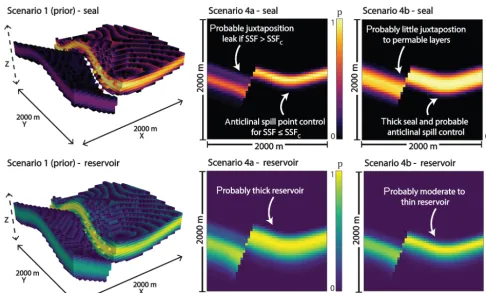
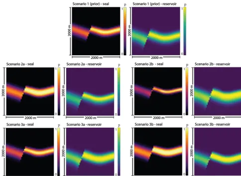
Figure 6.Probability field visualizations for seal and reservoir units in Scenarios 1 (prior), 4a, and 4b. For Scenario 1, we used 3-D voxel visualizations and set a threshold at a probability of 0.5 (only voxels with a probability higher than 0.5 are shown). It can be recognized that the seal is disrupted across the fault in more than 50 % of the prior model realizations. For the other scenarios, we show the full probability field for both units on a section through the middle of the model (y=500 m), parallel to thex–zplane.
the likelihood of a thick reservoir to the likelihood of a thick seal.
3.4 Introducing SSF likelihoods
We considered two SSF-related likelihood scenarios. In Sce-nario 4a, we implemented solely an SSF likelihood that was based on a narrow normal distribution (µ=5.1, σ=0.3) with a mean near the critical value SSFc=5. In Scenario 4b, we combined the likelihood of a thick seal (2a) with a likely moderate but reliable SSF value (SSF normal distribution with µ=2 and σ=0.3). Figure 6 illustrates the posterior situations well.
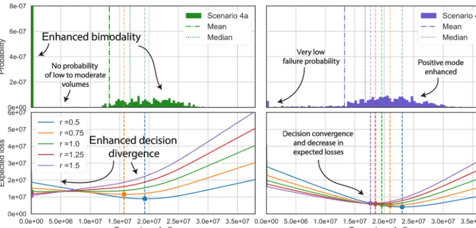
Scenario 4a resulted in increased bimodality of the pos-terior distribution (see Fig. 7). Accordingly, the Bayes ac-tion divergence and expected losses increased. Only two trap control mechanisms remained relevant for 4a (see Table B2): anticlinal spill (66 %) and cross-fault leakage to overlying formations (34 %).
The results for 4b were comparable to those of 2a but more pronounced. Entropies, particularly related to the seal thickness, were clearly reduced, also in the hanging wall. Probabilities of failure and low volumes were almost elimi-nated, further enhancing the highly positive mode. This
con-sequently resulted in an even higher convergence of Bayes actions, as well as reduction of expected losses compared to Scenario 2a. Anticlinal spill is the decisive control mecha-nism in 79.5 % of cases; otherwise, only cross-fault leakage to the reservoir occurred (20.5 %).
4 Discussion
Figure 7.Trap volume distribution and resulting loss function realizations for Scenario 4a and Scenario 4b. Adding a likelihood of the SSF being around its critical value led to increased bimodality and an elimination of low to moderate volume probabilities. Bayes actions diverged accordingly in Scenario 4a. Implementing a reliable SSF value likelihood (µ=2,σ=0.3) in combination with the thick seal likelihood from Scenario 2a resulted in an emphasis on highly positive volumes. This, in turn, led to a stark convergence of decisions and reduction of expected losses.
optimal decision. Given these aspects, we consider the use of custom loss functions with probabilistic geological mod-eling to be a very suitable combination in the framework of Bayesian decision theory.
The case study considered here addressed a typical sce-nario of exploration for a fluid reservoir. We first discuss ad-ditional relevant points with regard to this specific case and then provide more general comments on extensions and the application in additional fields in which geological models are commonly used.
4.1 State of knowledge, decision uncertainty, and consistent decision-making
As we defined trap volume to be in essence a determinis-tic function of uncertain model input parameters, uncertain-ties propagate to this parameter of interest when conduct-ing stochastic simulations. We consider the resultconduct-ing volume probability distributions to be expressions of the respective state of knowledge (or information) on which the decision-making is to be based. As this should include all parameters and conditions relevant for decision-making, we furthermore propose that the overall uncertainty inherent in this probabil-ity distribution can be referred to as “decision uncertainty” and that this entity should be viewed separately from geolog-ical model uncertainty.
By viewing decision-making as a problem of optimizing a case-specific custom loss function applied to such a state of knowledge and decision uncertainty, we were able to observe
clear differences in the respective behavior of distinctly risk-inclined actors.
The position and separation of their minimizing estima-tors, i.e., their decisions, manifested according to the proper-ties of the value distributions. The general spread and the oc-currence of modes relative to the overall distribution and the relevant decision space appear to be particularly significant. High spread and bimodal tendencies, i.e., high overall uncer-tainty, resulted in a wider separation of different actions. Re-duction of the distribution to one mode conversely led to their convergence. A decrease in decision uncertainty was further-more accompanied by a reduction in expected loss for each Bayes estimator.
Considering these observations, we derive the degree of action convergence and respective expected losses as mea-sures for the state of knowledge and decision uncertainty at the moment of making a decision. The better these are, the more similar the decisions of differently risk-inclined actors and the lower their loss expectations are. Given perfect in-formation all actors would bid on the same estimate (the true value) and expect no loss, since no risk would be present. It furthermore follows from this that the relevance of risk affin-ity decreases with greater reduction of decision uncertainty. 4.2 On the impact of additional information on
decision-making
We observed that the impact on decision uncertainty, in-duced by Bayesian inference, is not simply strictly aligned with the change in uncertainty regarding model parameters but on parameter combinations that are relevant for the out-come of the value of interest. It seems to be of central im-portance (1) “where” in the model uncertainty is reduced, i.e., in which spatial area or regarding which model parame-ters, and (2) which possible outcome is enhanced in terms of probability. An increased probability of a thick or thin seal in our model equally reduced decision uncertainty sig-nificantly by raising the probability of a positive or negative outcome, respectively. Improved certainty about our reser-voir thickness, however, had far lesser impact on decision-making. This shows that some areas and parameter combi-nations have a much greater influence on the decision uncer-tainty than others, depending on the way they contribute to the outcome of the value of interest.
Some types of additional information could even lead to increased decision uncertainty. We observed this in Sce-nario 4a. The introduced SSF likelihood practically con-strained our geological model to two possible situations: (1) a trap that is sealed off from juxtaposing layers and full to spill and (2) complete failure of the trap due to a breached seal across the fault. This made the decision problem a predomi-nantly binary one and split the outcome distribution into two narrowed but distant modes. The resulting increase in deci-sion divergence and expected losses show that, in some cases, adding information might leave actors in greater disagree-ment than before.
However, we furthermore have to consider that actors weight possible outcomes of the value distribution differ-ently. They are consequently affected differently by the same type of information. Risk-friendly actors were the most ro-bust in their decision-making in the face of possible trap failure. Eliminating this risk proved to be far less signifi-cant for the most risk-friendly than for risk-averse actors. Accordingly, it should be of foremost importance for risk-averse actors to reduce the uncertainty regarding critical fac-tors, such as seal integrity, which might decide between the success and complete failure of a project. This is less rele-vant for risk-friendly decisions makers, who might acquire a comparable benefit from knowing more about the probability of positive outcomes. They are less afraid of failure than they are of missing out on opportunity.
Crucial risks might be easily assessed if they are depen-dent on only one or a few parameters, such as seal thickness. In other cases, they are derived from more complex parame-ter inparame-terrelations, as is the case for the shale smear factor. To approach an effective mitigation of high risks, the complex-ities behind decisive factors need to be assessed thoroughly, and respective parent parameters, as well as their interde-pendencies, need to be identified. This might enable a better understanding of which type of information is missing and where in the model additional data might be of use for im-proved decision-making.
More of simply any type of information does not neces-sarily lead to better decisions. Instead, improved decision-making is achieved by attaining the right kind of information that is able to shed light on uncertainties that are relevant to an individual’s own goals and preferences, as well as the general problem at hand. Bratvold and Begg (2010) stated that value is not generated by uncertainty quantification or reduction in itself but is created to the extent that these pro-cesses have the potential to change a decision. Such deci-sion changes were clearly indicated by the shifting of ac-tions in our different scenarios. According to Hammitt and Shlyakhter (1999), the difference in expected payoff between the prior and posterior optimal decision gives the expected value of information. This raises the question of to what ex-tent a change in expected losses in itself might be an indicator for the value of information and if there is value in gaining confidence in a decision, even though it remains unchanged. 4.3 On the significance of our method in the
hydrocarbon sector
While Monte Carlo simulation is by now common in the hydrocarbon sector, it does not make decisions, as Murtha (1997) emphasized – it merely prepares for it. We believe that loss functions have the potential to go one step further. A hypothetical ideal loss function would consider all condi-tions in an economic environment, as well as perfectly repre-sent the preferences and goals of an actor and consequently be able to automatically find an optimal decision. While this is obviously unrealistic, we presume that an elaborate loss function might at least provide a very good preliminary deci-sion recommendation. It might furthermore be able to weight risks that are not immediately apparent to an individual as a person. Furthermore, the influence of human biases and psy-chological behavioral challenges, as described by Bratvold and Begg (2010), could be mitigated.
Bayesian inference and MCMC methods have been ap-plied for OOIP estimation and forecasting of reservoir pro-ductivity by Wadsley (2005), Ma et al. (2006), and Liu and McVay (2010). However, their research focused on history-matching simulations for already producing fields. Our ap-proach of applying Bayesian inference for structural geo-logical modeling and volumetric reservoir calculations is in-tended to support decision-making in the earliest stages of a reservoir when it has to be decided whether a project should be developed or not. Nevertheless, it was shown in the re-search conducted by Wadsley (2005) that early volumetric OOIP estimates can be combined with later calculations from production data via MCMC methods.
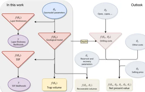
Figure 8.In this work, we applied our loss function approach to estimate a hydrocarbon trap volume. For this, we considered stochastic geomodeling parameters, defined deterministic functions to acquire volume, layer thicknesses, and SSF values, and linked the latter two to respective likelihoods. Regarding the bigger picture, this methodology is expandable and could include other parameters and dependencies. By taking into account other reservoir parameters and recovery factors, we could, for example, base decision-making on recoverable volumes. We could also take depth information from our model and combine this with other cost parameters to calculate drilling costs. Including additional costs, but also the selling price of hydrocarbons, we could attain the NPV as our final value of interest.
the size of a production platform. Based on such previously defined actual options, we could discretize our value prob-ability distribution into sections, which represent each deci-sion scenario accordingly. Our minimizing estimators would then indicate the best discrete option for a decision maker.
4.4 Extensions and outlook
We applied the concept of decision theory here to an implicit geological modeling method (de la Varga et al., 2019). De-pending on the application, other types of geometric inter-polations may be more suitable to represent the geological setting. More details on these methods, as well as the con-sideration of respective model uncertainties and the potential integration into probabilistic frameworks, are described, for example, in Wellmann and Caumon (2018).
We defined risk affinity to be dependent on arbitrarily cho-sen risk factors that led to according reweighting. Davidson-Pilon (2015) used risk parameters determined by the maxi-mal loss each actor could incur. Other approaches could be
based on more tangible values, for example by making risk attitude dependent on a fixed budget.
There are still many points that could be expanded on in future research. It would be of interest to apply the same overall concept and methodology to an authentic case based on real datasets. Given a realistic economic scenario includ-ing the capital and operational expenditures of a project, a full net-present-value (NPV) analysis could possibly be con-ducted by applying a loss function to an NPV distribution (see Fig. 8). A more elaborate loss function could be cus-tomized on the basis of surveys, thereby acquiring the spe-cific preferences of one or several companies and thus ob-taining a better profile of the economic environment, as well as the individuals acting in it.
exam-ple in groundwater extraction or geothermal energy usage. Also closely related are applications of fluid storage in sub-surface reservoirs, most prominently carbon capture and stor-age (CCS) applications. Questions regarding storstor-age capac-ity and safety deal with similar conditions and geological problems as the ones presented in this work. The described concepts can similarly be applied to other types of geologi-cal features, for example ore bodies in mineral exploration or subsurface structures and materials in geotechnical applica-tions. In all of these cases, the geological model can have sig-nificant uncertainties and, similar to the example described in this paper, further engineering and usage aspects carry high costs. We are therefore confident that a more detailed analysis of uncertainties and the definition and understand-ing of custom loss functions in the context of Bayesian deci-sion theory are very interesting paths for future research with wide possible applications.
Appendix A: Determination of the maximum trap volume
The volume is calculated on a voxel-count basis. To assign model voxels to the trap feature, it is necessary to check whether the following conditions (illustrated in Fig. 4) are satisfied by each individual voxel.
1. Labeled as reservoir formation.The voxel has been as-signed to the target reservoir formation (see Sandstone 1 in Fig. 4 (1)) in GemPy’s lithology block model. 2. Location above spill point horizon.The voxel is located
vertically above the final spill point of the trap. In the algorithm to find this final spill point, a spill point de-fined by the folding structure, referred to as an anticlinal spill point, and a cross-fault leak point that depends on the magnitude of displacement and the resulting nature of juxtapositions are distinguished. Once both of these points have been determined, the higher one is defined to be the final spill point used to determine the maxi-mum fill capacity of the trap. Given a juxtaposition with layers overlying the seal, due to fault displacement, the respective section is checked for fault sealing by taking into account the shale smear factor (SSF) value, which is the ratio of fault throw magnitude D to displaced shale thicknessT (Lindsay et al., 1993; Yielding et al., 1997; Yielding, 2012):
SSF=D
T . (A1)
We attain bothD andT by examining the contact be-tween the seal lithology voxels and the fault surface. For our model, we define the critical SSF to be SSFc= 5. We assume that cross-fault sealing is breached when this threshold is surpassed. For simplicity, the fault is considered to be sealing along its plane.
3. Location inside a closed system. The voxel is part of a model section inside the main anticlinal feature. All of the voxels inside this particular section are separated from the borders of the model by voxels that do not meet the first two conditions above, which primarily means that they are encapsulated by seal voxels upwards and laterally. This condition is relevant under the assump-tion that connecassump-tion to the borders of the model leads to leakage. A trap is thus defined as a closed system in this model and trap closure is assumed to be void outside the space of information, i.e., the model space. In our example model, this also means that hydrocarbons es-cape in the hanging wall due to respective layer dipping upwards towards the model borders.
It has to be emphasized that these conditions have been fitted to our synthetic example model. For other models featuring
different geological properties, structures, and levels of com-plexities, these conditions and respective algorithms might not apply. Models of higher complexities will surely require the introduction of further conditions.
A1 Anticlinal spill point detection
Regarding anticlinal structures and traps, it can be observed that, geometrically and mathematically, a spill point is a sad-dle point of the reservoir top surface in 3-D. This was de-scribed by Collignon et al. (2015), who pointed out that the linkage of folds is given by saddle points. These are thus a controlling factor for spill-related migration from respective structural traps. For anticlinal traps, closure can consequently be defined as the distance between the saddle point (i.e., spill point) and maximal point of the trap (Collignon et al., 2015). Regarding a surface defined by f (x, y), a local maxi-mum at(x0, y0, z0)would resemble a hilltop (Guichard et al., 2013). Local maxima will be found looking at the cross sec-tions in the planesy=y0andx=x0. Furthermore, the re-spective partial derivatives (i.e., gradients) δzδx and δzδy will equal zero at x0 and y0, i.e., the extremum is a stationary point (Guichard et al., 2013; Weisstein, 2017). In the context of a geological reservoir system, such a hill can be regarded as a representation of an anticlinal structural trap. Local min-ima are defined analogously, presenting local minmin-ima in both planes at a stationary point (Guichard et al., 2013). A saddle point, however, is a stationary point, while not being an ex-tremum (Weisstein, 2017). In general, saddle points can be distinguished from extrema by applying the second deriva-tive test (Guichard et al., 2013; Weisstein, 2017): considering a 2-D functionf (x, y)with continuous partial derivatives at a point(x0, y0)so thatfx(x0, y0)=0 andfx(x0, y0)=0, the following discriminantDcan be introduced:
D(x0, y0)=fxx(x0, y0)fyy(x0, y0)−fxy(x0, y0)2. (A2) Using this, the following holds for a point(x0, y0).
1. IfD >0 andfxx(x0, y0) <0, there is a local maximum. 2. IfD >0 andfxx(x0, y0) >0, there is a local minimum. 3. IfD <0, there is a saddle point at the point(x0, y0). 4. IfD=0, the test fails (Guichard et al., 2013).
According to Verschelde (2017), a saddle point in a matrix is maximal in its row and minimal in its column. This cor-responds to the logical geometrical deduction that a saddle point for a surface defined by f (x, y) is marked by a lo-cal maximum in one plane but a lolo-cal minimum in the per-pendicular plane. In our spill point detection algorithm, we make use of GemPy’s ability to return layer boundary sur-faces (simplices and vertices) as well as the gradients of the potential fields in discretized arrays.
2. Then, we check for the change in gradient sign at each such point in perpendicular directions. If they are oppo-site to one another, we can classify the vertex as a saddle point.
3. Lastly, we declare the highest saddle point to be our an-ticlinal spill point.
A2 Cross-fault leak point detection
For the potential point of leakage to formations underlying the seal across the normal fault (including the reservoir it-self), we take the highest zposition of the reservoir units’ contact (voxelized) with the fault in the hanging wall.
In the case of a juxtaposition with seal-overlying forma-tions and a failed SSF check, the maximum contact of the trap with the fault becomes the final spill point. Due to the shape of the trap in our model, we can then expect full leak-age and set the maximum trap volume to zero.
A3 Calculating the maximum trap volume
When all trap voxels have been determined via the condi-tions defined in Sect. 2.2.3, the maximum trap volumeVtis calculated by simply counting the number of trap voxels and rescaling their cumulative volume depending on the resolu-tion in which the model was computed:
Vt=nv· S
o Rm
3
, (A3)
wherenvis the number of trap voxels,Sogives the original scale, andRmis the resolution used for the model.
Appendix B: Results data
Table B1.Decision results for all considered scenarios and each actor. Respective optimal estimates (decisions) are represented byθ, whileˆ 1θˆindicates posterior changes relative to the prior (Scenario 1) result. Expected losses are given byl, and changes relative to the prior by
1l.
Decision makers
Risk friendly Risk neutral Risk averse
r=0.5 r=0.75 r=1.0 r=1.25 r=1.5
Scenario 1 θˆ 19 072 000.00 15 616 000.00 8 960 000.00 1 280 000.00 0.00
Prior l 8 582 112.55 10 785 632.54 12 100 484.80 11 759 772.46 10 763 671.94
Scenario 2a θˆ 22 528 000.00 19 712 000.00 17 920 000.00 16 448 000.00 15 232 000.00
Thick seal 1θˆ 3 456 000.00 4 096 000.00 8 960 000.00 15 168 000.00 15 232 000.00
l 5 387 582.96 6 654 239.73 7 544 384.00 8 220 155.30 8 776 678.80 1l −3 194 529.59 −4 131 392.81 −4 556 100.80 −3 539 617.16 −1 986 993.14
Scenario 2b θˆ 0.00 0.00 0.00 0.00 0.00
Thin seal 1θˆ −19 072 000.00 −15 616 000.00 −8 960 000.00 −1 280 000.00 0.00
l 2 743 719.13 2 240 237.29 1 940 102.40 1 735 280.34 1 584 086.98 1l −5 838 393.42 −8 545 395.25 −10 160 382.40 −10 024 492.12 −9 179 584.96
Scenario 3a θˆ 17 408 000 8 640 000 0 0 0
Thick reservoir 1θˆ −1 664 000.00 −6 976 000.00 −8 960 000.00 −1 280 000.00 0.00 l 10 073 515.53 12 159 993.48 11 319 609.6 10 124 566.62 9 242 422.54 1l 1 491 402.98 1 374 360.94 −780 875.20 −1 635 205.84 −1 521 249.40 Scenario 3c θˆ 22 784 000.00 20 096 000.00 18 432 000.00 16 960 000.00 15 680 000.00
Thick reservoir and seal 1θˆ 3 712 000.00 4 480 000.00 9 472 000.00 15 680 000.00 15 680 000.00 l 5 380 782.45 6 658 861.07 7 551 644.80 8 278 631.71 8 857 405.68 1l −3 201 330.10 −4 126 771.47 −4 548 840.00 −3 481 140.75 −1 906 266.26
Scenario 4a θˆ 19 264 000.00 15 744 000.00 0.00 0.00 0.00
Near-critical SSF 1θˆ 192 000.00 128 000.00 −8 960 000.00 −1 280 000.00 0.00
l 8 959 284.13 11 533 073.67 13 250 828.80 11 851 901.58 10 819 256.41
1l 377 171.58 747 441.13 1 150 344.00 92 129.12 55 584.47
Scenario 4b θˆ 23 040 000.00 20 992 000.00 19 584 000.00 18 496 000.00 17 664 000.00 Reliable SSF and thick seal 1θˆ 3 968 000.00 5 376 000.00 10 624 000.00 17 216 000.00 17 664 000.00 l 4 112 858.01 4 964 529.37 5 513 651.20 5 929 335.97 6 245 426.13 1l −4 469 254.54 −5 821 103.17 −6 586 833.60 −5 830 436.49 −4 518 245.81
Table B2.Occurrence rate of trap control mechanisms in percent for each information scenario.
1 – Anticlinal spill 2 – Leak to reservoir 3 – Leak to overlying 4 – Stratigraphic breach 5 – Unclear
Scenario 1 51.47 25.11 12.36 10.56 0.5
Scenario 2a 63.1 35.8 0.41 0.49 0.2
Scenario 2b 10.04 1.53 20.82 65.51 2.1
Scenario 3a 41.99 23.21 23.06 11.38 0.36
Scenario 3b 61.86 36.59 0.53 1.02 0
Scenario 4a 66.4 0.01 33.59 0 0
Appendix C: MCMC convergence
Author contributions. FAS, MdlV, and FW contributed to the con-ceptualization and method development. FAS designed the geolog-ical model, as well as the custom loss function, and conducted sim-ulations. FAS wrote and maintained the code with the help of MdlV (geological modeling with GemPy and simulations with PyMC). FAS prepared the article with contributions from both co-authors in reviewing and editing. MdlV was involved in creating some of the figures. FW conceived the original idea and provided scientific supervision and guidance throughout the project.
Competing interests. The authors declare that they have no conflict of interest.
Special issue statement. This article is part of the special issue “Understanding the unknowns: the impact of uncertainty in the geo-sciences”. It is a result of the EGU General Assembly 2018, Vienna, Austria, 8–13 April 2018.
Acknowledgements. We would like to thank Cameron Davidson-Pilon for his comprehensive, free introduction into Bayesian meth-ods, which inspired parts of this research. Special thanks to Alexan-der Schaaf for helping with 3-D visualizations. We would also like to acknowledge the funding provided by the DFG through DFG project GSC111.
Financial support. This research has been supported by the DFG (grant no. GSC111).
Review statement. This paper was edited by Lucia Perez-Diaz and reviewed by two anonymous referees.
References
Bardossy, G. and Fodor, J.: Evaluation of Uncertainties and Risks in Geology: New Mathematical Approaches for their Handling, Springer, Berlin, Germany, 2004.
Berger, J. O.: Statistical decision theory and Bayesian analysis, Springer Science & Business Media, New York, 2013.
Box, G. E. and Tiao, G. C.: Bayesian inference in statistical analy-sis, vol. 40, John Wiley & Sons, New York, 2011.
Bratvold, R. and Begg, S.: Making good decisions, Society of Petroleum Engineers, Richardson, TX, 2010.
Caers, J.: Modeling Uncertainty in the Earth Sciences, John Wiley & Sons, Ltd, Chichester, UK, 2011.
Calcagno, P., Chilès, J.-P., Courrioux, G., and Guillen, A.: Geolog-ical modelling from field data and geologGeolog-ical knowledge: Part I. Modelling method coupling 3D potential-field interpolation and geological rules, Phys. Earth Planet. In., 171, 147–157, 2008. Chatfield, C.: Model Uncertainty, Data Mining and Statistical
Infer-ence, J. R. Stat. Soc. A Stat., 158, 419–466, 1995.
Collignon, M., Fernandez, N., and Kaus, B.: Influence of surface processes and initial topography on lateral fold growth and fold linkage mode, Tectonics, 34, 1622–1645, 2015.
Davidson-Pilon, C.: Bayesian Methods for Hackers: Probabilistic Programming and Bayesian Inference, Addison-Wesley Profes-sional, Crawfordsville, Indiana, 2015.
Dean, L.: Reservoir Engineering for Geologists – Volumetric Es-timation, The Monthly Magazine of the Canadian Society of Petroleum Geologists, December Issue, 11–14, 2007.
de la Varga, M. and Wellmann, J. F.: Structural geologic modeling as an inference problem: A Bayesian perspective, Interpretation, 4, SM1–SM16, 2016.
de la Varga, M., Schaaf, A., and Wellmann, F.: GemPy 1.0: open-source stochastic geological modeling and inversion, Geosci. Model Dev., 12, 1–32, https://doi.org/10.5194/gmd-12-1-2019, 2019.
Gelman, A., Carlin, J. B., Stern, H. S., and Rubin, D. B.: Bayesian data analysis, vol. 2, Taylor & Francis, Boca Raton, FL, 2014. Geweke, J.: Evaluating the accuracy of sampling-based approaches
to the calculation of posterior moments, vol. 196, Federal Re-serve Bank of Minneapolis, Research Department Minneapolis, MN, USA, 1991.
Guichard, D., Koblitz, N., and Keisler, H. J.: Calculus: Early Tran-scendentals, D. Guichard, 2013.
Haario, H., Saksman, E., and Tamminen, J.: An adaptive metropo-lis algorithm, Bernoulli, Mathematical Reviews (MathSciNet), 7 223–242, 2001.
Hammitt, J. K. and Shlyakhter, A. I.: The expected value of infor-mation and the probability of surprise, Risk Analysis, 19, 135– 152, 1999.
Harney, H. L.: Bayesian inference: Parameter estimation and deci-sions, Springer Science & Business Media, Berlin, 2013. Hennig, C. and Kutlukaya, M.: Some Thoughts About the Design of
Loss Functions, REVSTAT – Statistical Journal, 5, 19–39, 2007. Jaynes, E. T.: Probability theory: The logic of science, Cambridge
University Press, Cambridge, UK, 2003.
Lajaunie, C., Courrioux, G., and Manuel, L.: Foliation fields and 3D cartography in geology: principles of a method based on potential interpolation, Math. Geol., 29, 571–584, 1997.
Lark, R., Mathers, S., Thorpe, S., Arkley, S., Morgan, D., and Lawrence, D.: A statistical assessment of the uncertainty in a 3-D geological framework model, Proceedings of the Geologists’ Association, 124, 946–958, 2013.
Lindsay, N., Murphy, F., Walsh, J., and Watterson, J.: Outcrop stud-ies of shale smears on fault surfaces, The Geological Modelling of Hydrocarbon Reservoirs and Outcrop Analogues, edited by: Flint, S. S. and Bryant, I. D., Special publication of the Inter-national Association of Sedimentologists, vol. 15, John Wiley & Sons Ltd., UK, pp. 113–123, 1993.
Liu, C. and McVay, D. A.: Continuous reservoir-simulation-model updating and forecasting improves uncertainty quantification, SPE Reserv. Eval. Eng., 13, 626–637, 2010.