Validation of the CrIS fast physical NH 3retrieval with ground-based FTIR

https://doi.org/10.5194/amt-10-2645-2017 © Author(s) 2017. This work is distributed under the Creative Commons Attribution 3.0 License.

Validation of the CrIS fast physical NH

3

retrieval

with ground-based FTIR

Enrico Dammers1, Mark W. Shephard2, Mathias Palm3, Karen Cady-Pereira4, Shannon Capps5,a, Erik Lutsch6, Kim Strong6, James W. Hannigan7, Ivan Ortega7, Geoffrey C. Toon8, Wolfgang Stremme9, Michel Grutter9, Nicholas Jones10, Dan Smale11, Jacob Siemons2, Kevin Hrpcek12, Denis Tremblay13, Martijn Schaap14, Justus Notholt3, and Jan Willem Erisman1,15

1_{Cluster Earth and Climate, Department of Earth Sciences, Vrije Universiteit Amsterdam, Amsterdam, the Netherlands} 2_{Environment and Climate Change Canada, Toronto, Ontario, Canada}

3_{Institut für Umweltphysik, University of Bremen, Bremen, Germany}

4_{Atmospheric and Environmental Research (AER), Lexington, Massachusetts, USA} 5_{Department of Mechanical Engineering, University of Colorado, Boulder, Colorado, USA} 6_{Department of Physics, University of Toronto, Toronto, Ontario, Canada}

7_{NCAR, Boulder, Colorado, USA}

8_{Jet Propulsion Laboratory, California Institute of Technology, Pasadena, California, USA}

9_{Centro de Ciencias de la Atmósfera, Universidad Nacional Autónoma de México, Mexico City, Mexico} 10_{University of Wollongong, Wollongong, Australia}

11_{National Institute of Water and Atmosphere, Lauder, New Zealand}

12_{University of Wisconsin-Madison Space Science and Engineering Center (SSEC), Madison, Wisconsin, USA} 13_{Science Data Processing, Inc., Laurel, MD, USA}

14_{TNO Built Environment and Geosciences, Department of Air Quality and Climate, Utrecht, the Netherlands} 15_{Louis Bolk Institute, Driebergen, the Netherlands}

a_{now at: Civil, Architectural, and Environmental Engineering Department, Drexel University,} Philadelphia, Pennsylvania, USA

Correspondence to:Enrico Dammers ([email protected]) Received: 6 February 2017 – Discussion started: 21 March 2017

Revised: 21 June 2017 – Accepted: 27 June 2017 – Published: 25 July 2017

Abstract. Presented here is the validation of the CrIS (Cross-track Infrared Sounder) fast physical NH3 retrieval (CFPR) column and profile measurements using ground-based Fourier transform infrared (FTIR) observations. We use the total columns and profiles from seven FTIR sites in the Network for the Detection of Atmospheric Composition Change (NDACC) to validate the satellite data products. The overall FTIR and CrIS total columns have a positive corre-lation of r=0.77 (N=218) with very little bias (a slope of 1.02). Binning the comparisons by total column amounts, for concentrations larger than 1.0×1016molecules cm−2, i.e. ranging from moderate to polluted conditions, the rel-ative difference is on average∼0–5 % with a standard de-viation of 25–50 %, which is comparable to the estimated

relative profile comparison differences are in the range of the estimated retrieval uncertainties. At the surface, where CrIS typically has lower sensitivity, it tends to overestimate in low-concentration conditions and underestimate in higher atmospheric concentration conditions.

1 Introduction

The disruption of the nitrogen cycle by the human creation of reactive nitrogen has created one of the major challenges for humankind (Rockström et al., 2009). Global reactive ni-trogen emissions into the air have increased to unsurpassed levels (Fowler et al., 2013) and are currently estimated to be four times larger than pre-industrial levels (Holland et al., 1999). As a consequence the deposition of atmospheric reac-tive nitrogen has increased causing ecosystems and species loss (Rodhe et al., 2002; Dentener et al., 2006; Bobbink et al., 2010). Ammonia (NH3) as fertilizer is essential for agricul-tural production and is one of the most important reactive ni-trogen species in the biosphere. NH3emission, atmospheric transport, and atmospheric deposition are major causes of eutrophication and acidification of soils and water in semi-natural environments (Erisman et al., 2008, 2011). Through reactions with sulfuric acid and nitric acid, ammonium ni-trate and ammonium sulfate are formed, which embody up to 50 % of the mass of fine-mode particulate matter (PM2.5) (Seinfeld and Pandis., 1988; Schaap et al., 2004). PM2.5has been associated with various health impacts (Pope III et al., 2002, 2009). At the same time, atmospheric aerosols impact global climate directly through their radiative forcing effect and indirectly through the formation of clouds (Adams et al., 2001; Myhre et al., 2013). By fertilizing ecosystems, depo-sition of NH3 and other reactive nitrogen compounds also plays a key role in the sequestration of carbon dioxide (Oren et al., 2001).

Despite the significance and impact of NH3 on the envi-ronment and climate, its global distribution and budget are still relatively uncertain (Erisman et al., 2007; Clarisse et al., 2009; Sutton et al., 2013). One of the reasons is that in situ measuring of atmospheric NH3at ambient levels is complex due to the sticky nature and reactivity of the molecule, lead-ing to large uncertainties and/or sampllead-ing artefacts with the currently used measuring techniques (von Bobrutzki et al., 2010; Puchalski et al., 2011). Measurements are also very sparse. Currently, observations of NH3are mostly available in north-western Europe and central North America, supple-mented by a small number of observations made in China (Van Damme et al., 2015b). Furthermore, there is a lack of detailed information on its vertical distribution as only a few dedicated airborne measurements are available (Nowak et al., 2007, 2010; Leen et al., 2013; Whitburn et al., 2015; Shep-hard et al., 2015). The atmospheric lifetime of NH3is rather short, ranging from hours to a few days. In summary, global

emission estimates have large uncertainties. Estimates of re-gional emissions attributed to source types that are differ-ent from the main regions are even more uncertain due to a lack of process knowledge and atmospheric levels (Reis et al., 2009).

Over the last decade the development of satellite observa-tions of NH3from instruments such as the Cross-track In-frared Sounder (CrIS, Shephard and Cady-Pereira, 2015), the Infrared Atmospheric Sounding Interferometer (IASI, Clarisse et al., 2009; Coheur et al., 2009; Van Damme et al., 2014a), the Atmospheric Infrared Sounder (AIRS, Warner et al., 2016) and the Tropospheric Emission Spectrometer (TES, Beer et al., 2008; Shephard et al., 2011) have shown the potential to improve our understanding of NH3 distribu-tion. Recent studies show the global distribution of NH3 mea-sured at a twice daily scale (Van Damme et al., 2014a, 2015a) can reveal seasonal cycles and distributions for regions where measurements were unavailable until now. Comparisons of these observations to surface observations and model simula-tions show underestimasimula-tions of the modelled NH3 concentra-tion levels, pointing to underestimated regional and naconcentra-tional emissions (Clarisse et al., 2009; Shephard et al., 2011; Heald et al., 2012; Nowak et al., 2012; Zhu et al., 2013; Van Damme et al., 2014b; Lonsdale et al., 2017; Schiferl et al., 2014, 2016; Zondlo et al., 2016). However, the overall quality of the satellite observations is still highly uncertain due to a lack of validation. The few validation studies showed a lim-ited vertical, spatial and or temporal coverage of surface ob-servations for a proper uncertainty analysis (Van Damme et al., 2015b; Shephard et al., 2015; Sun et al., 2015). A recent study by Dammers et al. (2016a) explored the use of Fourier transform infrared (FTIR-NH3, Dammers et al., 2015) ob-servations to evaluate the uncertainty of the IASI-NH3total column product. The study showed the good performance of the IASI-LUT (look-up table; Van Damme et al., 2014a) re-trieval with a high correlation (r∼0.8), but indicated an un-derestimation of around 30 % due to potential assumptions of the shape of the vertical profile (Whitburn et al., 2016; IASI-NN, neural network), uncertainty in spectral line parameters and assumptions on the distributions of interfering species. The study showed the potential of using FTIR observations to validate satellite observations of NH3, but also stressed the challenges of validating retrievals that do not provide the vertical measurement sensitivity, such as the IASI-LUT re-trieval. Since no IASI satellite averaging kernels are provided for each retrieval, and thus no information is available on the vertical sensitivity and/or vertical distribution of each sepa-rate observation, it is hard to determine the cause of the dis-crepancies between the observations.

in-put parameters. The quality of the retrieval has so far not been thoroughly examined in comparison to other observa-tions. Shephard and Cady-Pereira (2015) used Observing System Simulation Experiment (OSSE) studies to evaluate the initial performance of the CrIS NH3retrieval, and report a small positive retrieval bias of 6 % with a standard devi-ation of ±20 % (ranging from±12 to±30 % over the ver-tical profile). Note that no potential systematic errors were included in these OSSE simulations. Their study also shows good qualitative comparisons with the Tropospheric Emis-sion Spectrometer (TES) satellite (Shephard et al., 2011) and the ground-level in situ quantum cascade laser (QCL) obser-vations (Miller et al., 2014) for a case study over the Central Valley in CA, USA, during the DISCOVER-AQ campaign. However, currently there has not been an extensive validation of the CrIS NH3retrievals using direct comparisons with ver-tical profile observations. In this study we will provide both direct comparisons of the CrIS-retrieved profiles and ground-based FTIR observations as well as comparisons of CrIS total column values and the FTIR and IASI.

2 Methods

2.1 The CrIS fast physical retrieval

CrIS was launched in late October 2011 on board the Suomi NPP platform. CrIS follows a sun-synchronous orbit with a daytime overpass time at 13:30 LT (local time) (ascending) and a night-time equator overpass at 01:30 LT. The instru-ment scans along a 2200 km swath using a 3×3 array of circular-shaped pixels with a diameter of 14 km at nadir for each pixel, which become larger ovals away from nadir. In this study we use the NH3 retrieval as described by Shep-hard and Cady-Pereira (2015). The retrieval is based on an optimal estimation approach (Rodgers, 2000) that minimizes the differences between CrIS spectral radiances and simu-lated forward model radiances computed from the Optimal Spectral Sampling method (OSS) OSS-CrIS (Moncet et al., 2008), which is built from the well-validated Line-By-Line Radiative Transfer Model (LBLRTM) (Clough et al., 2005; Shephard et al., 2009; Alvarado et al., 2013) and uses the HITRAN database (Rothman et al., 2013) for its spectral lines. The fast computational speed of OSS facilitates the operational production of CrIS-retrieved (level 2) products using an optimal estimation retrieval approach (Moncet et al., 2005). The CrIS OSS radiative transfer forward model computes the spectrum for the full CrIS LW band, at the CrIS spectral resolution of 0.625 cm−1 (Tobin, 2012); thus the complete NH3spectral band (near 10 µm) is available for the retrievals. However, only a small number of microwin-dows are selected for the CrIS retrievals to both maximize the information content and minimize the influence of er-rors. Worden et al. (2004) provides an example of a robust spectral region selection process that takes into consideration

both the estimated errors (i.e. instrument noise, spectroscopy errors, interfering species, etc.) and the associated informa-tion content in order to select the optimal spectral regions for the retrieval. The a priori profiles selection for the opti-mal estimation retrievals follows the TES retrieval algorithm (Shephard et al., 2011). Based on the relative NH3signal in the spectra the a priori is selected from one of three possi-ble profiles representing unpolluted, moderate, and polluted conditions. The initial guess profiles are also selected from these three potential profiles.

An advantage of using an optimal estimation retrieval ap-proach is that averaging kernels (sensitivity to the true state) and the estimated errors of the retrieved parameter are com-puted in a robust and straightforward manner (for more de-tails see Shephard and Cady-Pereira, 2015). The total satel-lite retrieved parameter error is expressed as the sum of the smoothing error (due to unresolved fine structure in the pro-file), the measurement error (random instrument noise in the radiance spectrum propagated to the retrieval parame-ter), and systematic errors from uncertainties in the non-retrieved forward model parameters and cross-state errors propagated from retrieval to retrieval (i.e. major interfering species such as H2O, CO2, and O3) (Worden et al., 2004). As of yet we have not included error estimates for the sys-tematic errors. The CrIS smoothing error is computed, but since in these FTIR comparison results we apply the FTIR observational operator (which accounts for the smoothing er-ror), the smoothing error contribution is not included in the CrIS errors reported in the comparisons. Thus, only the mea-surement errors are reported for observations used here; these errors can thus be considered the lower limit of the total esti-mated CrIS retrieval error.

Figure 1 shows an example of CrIS NH3observations sur-rounding one of the ground-based FTIR instruments. This is a composite map of all days in Bremen with observations in 2015. This figure shows the widespread elevated amounts of NH3across north-western Germany as observed by CrIS. Since the goal of this analysis is to evaluate the CrIS re-trievals that provide information beyond the a priori, we only performed comparisons when the CrIS spectrum presents a NH3 signal. We also focused our efforts on FTIR stations that have FTIR observations with total columns larger than 5×1015molecules cm−2(∼1–2 ppb surface VMR (volume mixing ratio). This restriction does mean that a number of sites of the FTIR-NH3 data set will not be used. For com-parability of this study to the results of the IASI-LUT eval-uation in an earlier study by Dammers et al. (2016a) we in-clude a short paragraph on the performance of the IASI-LUT and the more recent IASI-NN product when applying similar constraints.

2.2 FTIR-NH3retrieval

Table 1.The location, longitudinal and latitudinal position, altitude above sea level, and type of instrument for each of the FTIR sites used in this study. In addition, a reference is given to a detailed site description, when available.

Station Lon Lat Altitude FTIR instrument Reference (degrees) (degrees) (m a.s.l)

Bremen, Germany 8.85◦E 53.10◦N 27 Bruker 125 HR Velazco et al. (2007)

Toronto, Canada 79.60◦W 43.66◦N 174 ABB Bomem DA8 Wiacek et al. (2007) Lutsch et al. (2016) Boulder, USA 105.26◦W 39.99◦N 1634 Bruker 120 HR

Pasadena, USA 118.17◦W 34.20◦N 350 MkIV_JPL

Mexico City, Mexico 99.18◦W 19.33◦N 2260 Bruker Vertex 80 Bezanilla et al. (2014) Wollongong, Australia 150.88◦E 34.41◦S 30 Bruker 125 HR

Lauder, New Zealand 169.68◦E 45.04◦S 370 Bruker 120 HR Morgenstern et al. (2012)

Figure 1.Annual mean of the CrIS-retrieved NH₃ surface VMR values around the Bremen FTIR site for 2015. The two circles show the collocation area when for radii of 25 and 50 km.

on the retrieval methodology described by Dammers et al. (2015). The retrieval methodology uses two spectral mi-crowindows with spectral width that depends on the NH3 background concentration determined for the observation stations and location (wider window for stations with back-ground concentrations less than one ppb). NH3is retrieved by fitting the spectral lines in the two microwindows MW1 [930.32–931.32 cm−1 or wide: 929.40–931.40 cm−1] and MW2 [962.70–970.00 cm−1or wide: 962.10–970.00 cm−1]. An optimal estimation approach (Rodgers, 2000) is used, im-plemented in the SFIT4 algorithm (Pougatchev et al., 1995; Hase et al., 2004, 2006). There are a number of species that can interfere to some extent in both windows, with the ma-jor species being H2O, CO2and O3 and the minor species N2O, HNO3, CFC-12, and SF6. The HITRAN 2012 database

(Rothman et al., 2013) is used for the spectral lines. A further set of spectroscopic line parameter adjustments are added for CO2 taken from the ATMOS database (Brown et al., 1996) as well as a set of pseudo-lines for the broad absorptions by the CFC-12 and SF6molecules (created by NASA-JPL, G.C. Toon, http://mark4sun.jpl.nasa.gov/pseudo.html). The NH3 a priori profiles are based on balloon measurements (Toon et al., 1999) and refitted to match the local surface con-centrations (depending on the station either measured or es-timated by model results). For the interfering species a priori profiles we use the Whole Atmosphere Community Climate Model (WACCM, Chang et al., 2008, v3548). The estimated errors in the FTIR-NH3retrievals are of the order of∼30 % (Dammers et al., 2015) with the uncertainties in the NH3line spectroscopy being the most important contributor. Based on the data requirements in Sect. 2.1, a set of seven stations is used (Table 1). For all sites except Wollongong in Australia we use the basic narrow spectral windows. For Wollongong the wide spectral windows are used. For a more detailed de-scription of each of the stations see the publications listed in Table 1 or Dammers et al. (2016a).

2.3 IASI-NH3

Table 2. Coincidence criteria and quality flags applied to the satellite and FTIR data. The third through fifth columns show the number of observations remaining after each subsequent data criteria step and the number of possible combinations between the CrIS and FTIR observations. The first set of numbers indicate the number of CrIS observations within a 1◦×1◦degree square surrounding the FTIR site.

Filter Data criteria No. obs.

FTIR CrIS Combinations

CrIS 15 661 25 855

Temporal sampling difference Max 90 min 1576 13 959 112 179 Spatial sampling difference Max 50 km 1514 3134 22 869 Elevation difference Max 300 m 1505 1642 9713 Quality flag DOFS≥0.1 1433 1453 8579

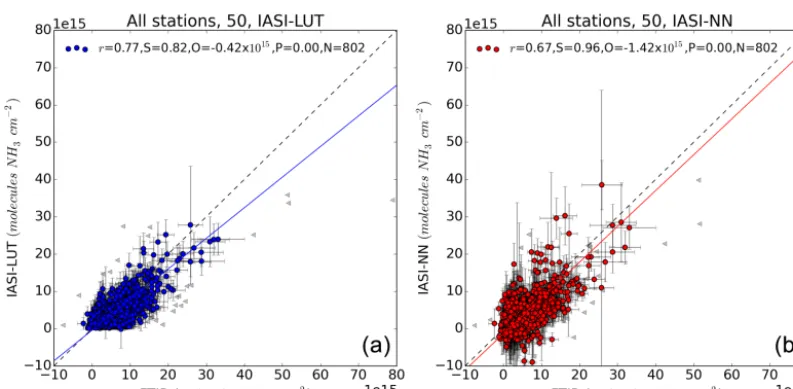
index (HRI) (Van Damme et al., 2014a). The HRI is repre-sentative of the amount of NH3in the measured column. The IASI-LUT retrieval makes a direct conversion of the HRI to total column density with the use of a look-up table (LUT). The LUT is created using a large number of simulations for a wide range of atmospheric conditions which link the ther-mal contrast (TC, the difference between the air temperature at 1.5 km altitude and the temperature of the Earth’s surface) and the HRI to a NH3total column density. The retrieval in-cludes a retrieval error based on the uncertainties in the initial HRI and TC parameters. The more recent IASI-NN retrieval (Whitburn et al., 2016) follows similar steps but it makes use of a neural network. The neural network combines the com-plete temperature, humidity and pressure profiles for a better representation of the state of the atmosphere. At the same time the retrieval error estimate is improved by including er-ror terms for the uncertainty in the profile shape, and the full temperature and water vapour profiles. The IASI-NN version uses the fixed profiles that were described by Van Damme et al. (2014a) but allows for the use of third party profiles to improve the representation of the NH3atmospheric profile. The IASI-LUT and IASI-NN retrievals have both been pre-viously compared with FTIR observations (Dammers et al., 2016a, b). They compared reasonably well with correlations aroundr=0.8 for a set of FTIR stations, with an underesti-mation of around 30 % that depends slightly on the magni-tude of total column amounts, with the IASI-NN performing slightly better.

2.4 Data criteria and quality

NH3 concentrations show large variations both in space and time as a result of the large heterogeneity in emis-sion strengths due to spatially variable sources and drivers such as meteorology and land use (Sutton et al., 2013). This high variability poses challenges in matching ground-based point observations made by FTIR observations with CrIS downward-looking satellite measurements which have a 14 km nadir footprint. For the pairing of the measurement data we apply data selection criteria similar to those de-scribed in Dammers et al. (2016a) and summarized in Ta-ble 2. To minimize the impact of the heterogeneity of the

sources, we choose a maximum of 50 km between the cen-tre points of the CrIS observations and the FTIR site loca-tion. To diminish the effect of temporal differences between the FTIR and CrIS observations, a maximum time differ-ence of 90 min is used. Topographical effects are reduced by choosing a maximum altitude difference of 300 m at any point between the FTIR site location and the centre point of the satellite pixel location. The altitude differences are cal-culated using the Space Shuttle Radar Topography Mission Global product at 3 arc-second resolution (SRTMGL3, Farr et al., 2007). To ensure the data quality of CrIS-NH3retrieval for version 1.0, a small number of outliers with a maximum retrieved concentration above 200 ppb (at any point in the profile) were removed from the comparison data set. While potentially a surface NH3 value of 200 ppb (and above) is possible (i.e. downwind of forest fires), it is highly unlikely to occur over the entire footprint of the satellite instrument. Moreover, after inspecting these data points, they seem to be affected by numerical issues in the fitting procedure (possibly due to interfering species). As we are interested in validating the CrIS observational information (not just a priori tion), we only select comparisons that contain some informa-tion from the satellite (degrees of freedom for signal – DOFS – ≥0.1). Do note that on average the observations have a DOFS between 0.9 and 1.1. The DOFS>0.1 filter only re-moves some of the outliers at the lower end. No explicit filter is applied to account for clouds; however, clouds will implic-itly be accounted for by quality control as CrIS will not mea-sure a NH3 signal (e.g. DOFS<0.1) below optically thick clouds (e.g. cloud optical depth>∼1). In addition, the CrIS observations are matched with FTIR observations taken only during clear-sky conditions, which mostly eliminates influ-ence from cloud cover. Finally, the high signal-to-noise ra-tios (SNR) of the CrIS instrument allows it to retrieve NH3 from a thermal contrast approaching 0 K during daytime ob-servations (Clarisse et al., 2010). Given this, we decided not to apply a thermal contrast filter to the CrIS data. No addi-tional filters are applied to the FTIR observations beyond the clear-sky requirement.

set of criteria is similar to those used here for the CrIS obser-vations. Observations from both IASI retrievals are matched using the overpass time, and longitudinal and latitudinal po-sitions. For comparability with CrIS a spatial difference limit of 50 km limit was used, instead of the 25 km spatial limit used in the previous study. Furthermore we apply the ther-mal contrast (>12 K, difference between the temperatures at 1.5 km and the surface) and Earth’s skin temperature criteria to the IASI observations to match the previous study.

2.5 Observational operator application

To account for the vertical sensitivity and the influence of the a priori profiles of both retrievals, we apply the observational operator (averaging kernel and a priori of the retrieval) of the FTIR retrieval to the CrIS-retrieved profiles. The CrIS ob-servations are matched to each individual FTIR observation in time and space following the matching criteria. The FTIR averaging kernels, a priori profiles and retrieved profiles are first mapped to the CrIS pressure levels (fixed pressure grid, layers are made smaller or cut off for observations above el-evation to fit the fixed pressure grid). Following Rodgers and Connor (2003) and Calisesi et al. (2005) this results in the mapped FTIR averaging kernel,Amapped_ftir , the mapped FTIR a priori,xmapped_ftir ,apriori, and the mapped FTIR-retrieved pro-file,xmapped_ftir . Then we apply the FTIR observational operator to the CrIS observations using Eq. (1).

ˆ

xCrIS=xmapped_ftir ,apriori+Amapped_ftir

xCrIS−xmapped_ftir ,apriori

(1)

ˆ

1xabs= ˆxCrIS−x mapped

ftir (2)

ˆ

1xrel=

ˆ

xCrIS−xmapped_ftir

/05xmapped_ftir +0.5· ˆxCrIS

, (3) wherexapriori_ftir is the FTIR a priori profile,xmapped_ftir is the inter-polated FTIR profile,Amapped_ftir is the FTIR averaging kernel, andxˆCrISis the smoothed CrIS profile.

The CrIS smoothed profile xˆCrIS calculated from Eq. (1) provides an estimate of the FTIR retrieval applied to the CrIS satellite profile. Next we evaluate both total column and pro-file measurements.

For the first validation step, following Dammers et al. (2016a), who evaluated the IASI-LUT (Van Damme et al., 2014a) product, we sum the individual profile (xˆCrIS) to obtain a column total to compare to the FTIR total columns. This step gives the opportunity to evaluate the CrIS retrieval in a similar manner as was done with the IASI-LUT retrieval. If multiple FTIR observations match a single CrIS overpass we also average those together into a single value as well as each matching averaged CrIS observation. Therefore, it is possible to have multiple FTIR observations, each with mul-tiple CrIS observations all averaged into a single matching representative observation. For the profile comparison this averaging is not performed to keep as much detail available

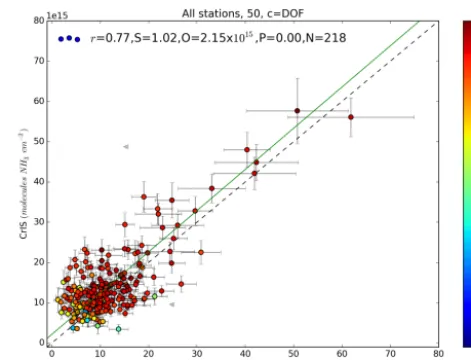
Figure 2.Correlation between the FTIR and CrIS total columns using the coincident data from all measurement sites. The horizontal and vertical bars show the total estimated error on each FTIR and CrIS observation. The colouring on the scatter indicates the mean DOF of each the CrIS coincident data. The trend line shows the results of the regression analysis.

as possible. An important point to make is that this approach assumes that the FTIR retrieval gives a better representation of the truth. While this may be true, the FTIR retrieval will not match the truth completely. For readability we assume that the FTIR retrieval indeed gives a better representation of the truth, and in the next sections we will describe the case in which we apply the FTIR observational operator to the CrIS values. For the tenacious reader we included a similar set of results in the appendix, using the CrIS observational operator instead of the FTIR observational operator, as the assumption of the FTIR being true is not exactly right.

3 Results and discussion

3.1 Total column comparison

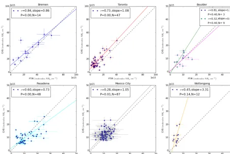
Figure 3.FTIR vs. CrIS comparison scatter plots showing the correlations for each of the individual stations, with estimates of error plotted for each value. The trend lines show the individual regression results. Note the different ranges on the xandyaxis. The results for the Boulder (green line) and Lauder (pink line) sites are shown in the same panel.

Figure 3 shows the comparisons at each station. When the comparisons are broken down by station (Fig. 3), the corre-lation varies from site to site, from a minimum of 0.28 in Mexico City (possibly due to retrieval errors associated with the highly irregular terrain) to a maximum of 0.84 in Bre-men. Similarly to Mexico City the comparison also shows an increase in scatter for Pasadena, where the FTIR site is also located on a hill. In Toronto and Bremen there is good agree-ment when NH3 is elevated (>20×1015molecules cm−2), and low bias in the CrIS total columns for intermediate val-ues (between 10 and 20×1015molecules cm−2) except for the outlying observation in Bremen, which is marked as an outlier by our 3σ filter used for Fig. 2. In Wollongong, there is less agreement between the instruments. There are two comparisons with large CrIS to FTIR ratios while most of the other comparisons also show a bias for CrIS. For both cases the bias can be explained by the heterogeneity of the ammonia concentrations in the surrounding regions. The two outlying observations were made during the end of Novem-ber 2012, which coincides with wildfires in the surrounding region. Furthermore the Wollongong site is located on the coast, which will increase the occurrences in which one in-strument observes clean air from the ocean while the other observes inland air masses.

The mean absolute (MD) and relative difference (MRD) are calculated following Eqs. (4) and (5);

MRD= 1

N N

X

i=1

(CrIS columni−FTIR columni)×100 0.5×FTIR columni+0.5×CrIS columni (4) MD= 1

N

N X

i=1

(CrIS columni−FTIR columni) (5)

withNbeing the number of observations.

Table 3. Results of the total column comparisons of the FTIR to CrIS, FTIR to IASI-LUT and FTIR to IASI-NN. N is the num-ber of averaged total columns, MD is the mean difference [1015molecules cm−2], MRD is the mean relative difference [frac, in %]. Take note that the combined value N does not add up with all the separate sites as observations have been included for FTIR total columns>5×1015molecules cm−2.

Retrieval Column total range N MD in 1015 MRD in % FTIR mean in in molecules cm−2 (1σ) (1σ) 1015(1σ)

CrIS-NH3 <10.0×1015 93 3.3 (4.1) 30.2 (38.0) 7.5 (1.5) CrIS-NH3 >=10.0×1015 109 0.4 (5.3) −1.39 (34.4) 16.7 (8.5) IASI-LUT <10.0×1015 229 −2.7 (3.0) −63.6 (62.6) 7.1 (1.4) IASI-LUT >=10.0×1015 156 −5.1 (4.2) −50.2 (43.6) 14.8 (6.7) IASI-NN <10.0×1015 212 −2.2 (3.6) −57.0 (68.7) 7.1 (1.4) IASI-NN >=10.0×1015 156 −5.0 (5.1) −52.5 (49.7) 14.8 (6.7)

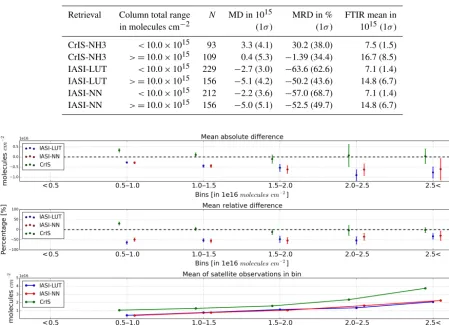
Figure 4.Plots of the mean absolute and relative differences between CrIS and IASI, as a function of NH3total column. Observations are separated into bins of total columns. Panel(a)shows the mean absolute difference (MD). Panel(b)shows the mean relative difference. The bars in these top two panels show the 95 % confidence interval for each value. Panel(c)shows the mean of the observations in each bin. The number of observations in each set is shown in the bottom panel.

the relative difference is applied to remove these outliers (<10×1015molecules cm−2, only the IASI-NN set). The statistical values are not given separately by site because of the low number of matching observations for a number of the sites.

The CrIS/FTIR comparison results show a large positive difference in both the absolute (MD) and relative (MRD) for the smallest bin, (5.0–10.0×1015molecules m−2). The rest of the CrIS/FTIR comparison bins with NH3 val-ues>10.0×1015 agree very well with a nearly constant bias (MD) around zero, and a standard deviation of the or-der of 5.0×1015, which slightly dips below zero in the mid-dle bin. The standard deviation over these bins is also more or less constant, and the weak dependence on the number of observations in each bin indicates that most of the effect is coming from the random error on the observations. The relative difference becomes systematically smaller with

in-creasing column total amounts, and tends towards zero with a standard deviation∼25–50 %, which is on the order of the reported estimated errors of the FTIR retrieval (Dammers et al., 2015).

func-tion of the total column. However, the relative differ-ence (MRD) is at its maximum for the smaller bin with a dif-ference of the order−50 % (std= ∼ ±50 %,N=229) which decreases to∼ −10–25 % (std= ±25 %) with increasing bin value. For both the IASI-NN and IASI-LUT retrievals we find an underestimation of the total columns, which origi-nates mostly from a large systematic error in combination with more randomly distributed error sources such as the instrument noise and interfering species, which are similar to results reported earlier for IASI-LUT (Dammers et al., 2016b).

A number of factors, besides the earlier reported FTIR un-certainties, can explain the differences between the FTIR and CrIS measurements. The small positive bias found for CrIS points to a small systematic error. The higher SNR, from both the low radiometric noise and high spectral resolution, en-ables it to resolve smaller gradients in the retrieved spectra, which can potentially provide greater vertical information and detect smaller column amounts (lower detection limit). This could explain the larger MRD and MD CrIS differences at the lower end of the total column range. However, a num-ber of standalone tests with the FTIR retrieval showed only a minor increase in the total column following a decrease in spectral resolution, which indicates that the spectral resolu-tion itself is not enough to explain the difference.

3.2 Profile comparison

The CrIS-satellite- and FTIR-retrieved profiles are matched using the criteria specified above in Table 2 and compared. It is possible for a CrIS observation to be included multiple times in the comparison as there can be more than one FTIR observation per day, and/or, the possibility of multiple satel-lite overpasses that match a single FTIR observation.

3.2.1 A representative profile example

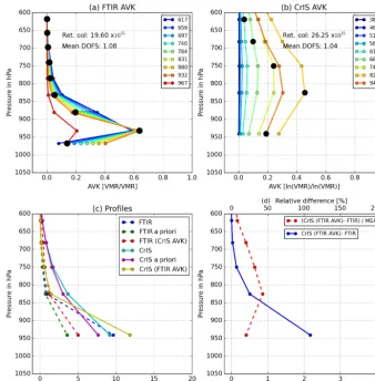
An example of the profile information contained in a repre-sentative CrIS and FTIR profile is shown in Fig. 5. Although the vertical sensitivity and distribution of NH3 differs per station this is fairly representative. The FTIR usually has a somewhat larger DOFS of the order of 1.0–2.0, mostly de-pending on the concentration of NH3compared to the CrIS total of ∼1 DOFS. Figure 5a shows an unsmoothed FTIR averaging kernel [vmr vmr−1] of a typical FTIR observation. The averaging kernel (AVK) peaks between the surface and

∼850 hPa, which is typical for most observations. In spe-cific cases with plumes passing over the site, the averaging kernel peak is at a higher altitude, matching the location of the NH3 plume. The CrIS averaging kernel (Fig. 5b) usu-ally has a maximum somewhere in between 680 and 850 hPa depending on the local conditions. This particular observa-tion has a maximum near the surface, an indicaobserva-tion of a day with high thermal contrast. Both the FTIR and CrIS concen-tration profiles have a maximum at the surface with a

con-tinuous decrease that mostly matches the a priori profile in a shape following the low DOFS. This is visible for layers at the lower pressures (higher altitudes) where the FTIR and CrIS a priori and retrieved volume mixing ratios become sim-ilar and near zero. The absolute difference between the FTIR and CrIS profiles can be calculated by applying the FTIR observational operator to the CrIS profile, as we described in Sect. 2.5. The largest absolute difference (Fig. 5d) is found at the surface, which is also generally where the largest absolute NH3 values occur. The FTIR smoothed relative difference (red, striped line) peaks at the pressure where the sensitivity of the CrIS retrieval is highest (∼55 %), which goes down to

∼20–30 % for the higher altitude and surface pressure lay-ers. Overall the retrievals agree with most of the difference explained by the estimated errors of the individual retrievals. For an illustration of the systematic and random errors on the FTIR and CrIS profiles shown in Fig. 5; see the figures in the Appendix. For the FTIR error profile see Fig. A2 (ab-solute error) and Fig. A3 (relative error) and for the CrIS measurement error profile see Fig. A4. Please note that we only show the diagonal error covariance values for each of the errors, which is common practice. The total column of our example profile is∼20×1015molecules cm−2which is a slightly larger value than average. The total random error is<10 % for each of the layers, mostly dominated by the measurement error, which is somewhat smaller than average (Dammers et al., 2015) following the larger NH3VMR. A similar value is found for the CrIS measurement error with most layers showing an error<10 %. The FTIR systematic error is around∼10 % near the surface and grows to 40 % for the layers between 900 and 750 hPa. The error is mostly due to the errors in the NH3spectroscopy (Dammers et al., 2015). The shape of the relative difference between the FTIR and CrIS closely follows the shape systematic error on the FTIR profile, pointing to that error as the main cause of dif-ference.

3.2.2 All paired data

Figure 5.Example of the NH₃profile comparison for an FTIR profile matched with a CrIS profile measured around the Pasadena site. With (a)the FTIR averaging kernel,(b)the CrIS averaging kernel. For both averaging kernels the black dots show the matrices diagonal values. (c)shows the retrieved profiles of both FTIR (blue) and CrIS (cyan) with the FTIR values mapped to the CrIS pressure layers. Also shown are the FTIR a priori (green), the CrIS a priori (purple), the CrIS-retrieved profile smoothed with the FTIR averaging kernel [CrIS (FTIR AVK)] (yellow) and the FTIR profile smoothed with the CrIS averaging kernel [FTIR (CrIS AVK)](red). In(d), the blue line is the absolute difference between the FTIR profile (blue,c) and the CrIS profile smoothed with the FTIR averaging kernel (yellow,c) with the red line as the corresponding relative difference.

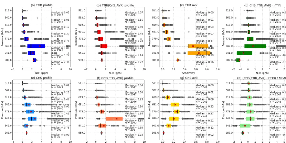
of observations used in the box plot, many with weak sensi-tivity at the surface. Similar to the single profile example in Fig. 5, the FTIR averaging kernels in Fig. 6c peak on average near or just above the surface (with the diagonal elements of the AVK’s shown in the figure). The sensitivity varies a great deal between the observations as shown by the large spread of the individual layers. The CrIS averaging kernels (Fig. 6g) usually peak in the boundary layer around the 779 hPa layer with the two surrounding layers having somewhat similar values. The instrument is less sensitive to the surface layer as is demonstrated by the large decrease in the AVK near the surface, but this varies depending on the local conditions. We find the largest absolute differences in the lower three layers, as was seen in the example in Fig. 5, although the differences decrease rather than increase. The relative difference shows

Figure 6.Profile comparison for all stations combined. Observations are combined following pressure “bins”, i.e. the midpoints of the CrIS pressure grid. Panel(a)shows the mean profiles of the FTIR (blue),(b)the profiles of FTIR with the CrIS averaging kernel applied to it (red),(c)the FTIR averaging kernel diagonal values, and(d)shows the absolute difference [VMR] between profiles(f)and(a). The second row shows the CrIS mean profile in (e),(f) shows the profiles of CrIS with the FTIR averaging kernel applied,(g)the CrIS averaging kernel diagonal values,(h)the relative difference [Fraction] between the profiles in(f)and(a). Each of the boxes edges are the 25th and 75th percentiles, the black lines in each box is the median, the red square is the mean, the whiskers are the 10th and 90th percentiles, and the grey circles are the outlier values outside the whiskers.

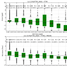
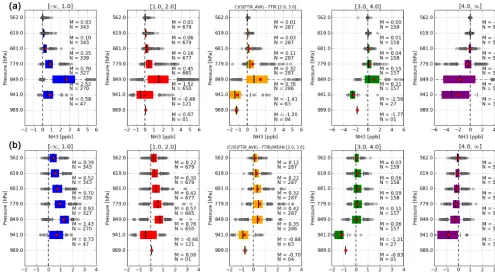
The switch between negative and positive values in the absolute difference (see Fig. 6d) occurs in the two lowest layers dominated by the Bremen observations and provides insight into the relation between absolute differences as a function of retrieved concentration. Figure 7 shows a sum-mary of the differences as a function of the individual NH3 VMR layer amounts. As seen before in the column compar-ison, e.g. Figs. 2 and 4, the CrIS retrieval gives larger to-tal columns than the FTIR retrieval for the small values of VMR. For increasing VMRs, this slowly tends to a negative absolute difference with a relative difference in the range of 20–30 %. However, note that the number of compared val-ues in these high VMR bins are by far lower than in the first three bins leading to a relatively smaller effect in the total column and merged VMR figures (Figs. 2 and 6) from these high VMR bins. We now combine the results of Figs. 6 and 7 with Fig. 8 to create a set of subplots showing the dif-ference between both retrieved profiles as a function of the maximum VMR of each retrieved FTIR profile. For the lay-ers with pressure less than 681 hPa we generally find agree-ment, which is expected but not very meaningful, since there is not much NH3(and thus sensitivity) in these layers and any differences are smoothed out by the application of the observational operator. The relative differences for these lay-ers all lie around ∼0–20 %. For the lowest two VMR bins

Figure 7.Summary of the absolute and relative actual error as a function of the VMR of NH3 in the individual FTIR layers. The box edges are the 25th and 75th percentiles, the black line in the box is the median, the red square is the mean, the whiskers are the 10th and 90th percentiles, and the grey circles are the outlier values outside the whiskers. Only observations with a pressure greater than 650 hPa are used. The top panel shows the absolute difference for each VMR bin, the bottom panel shows the relative difference for each VMR bin.

is chosen following a selection based on the strength of NH3 signature in the spectra. The three a priori profiles (unpol-luted, moderately polluted and polluted) are different in both shape and concentration. Out of the entire set of 2047 com-binations used in Fig. 8, only six are from the non-polluted a priori category. About one-third of the remaining obser-vations use the polluted a priori, which has a sharper peak near the surface (see Fig. 5c) compared to the moderately polluted profile, which is used by two-thirds of the CrIS re-trievals shown in this work. Based on the results as a func-tion of retrieved VMR (as measured with the FTIR so not a perfect restriction), it is possible that the sharper peak at the surface as well as the low a priori concentrations are re-stricting the retrieval. The dependence of the differences on VMR can also possibly follow from uncertainties in the line spectroscopy. In the lower troposphere there is a large gra-dient in pressure and temperature and the impact of any un-certainty in the line spectroscopy is greatly enhanced. Even for a day with large thermal contrast and NH3concentrations (e.g. Fig. 5), the difference between both the CrIS and FTIR retrievals was dominated by the line spectroscopy. This ef-fect is further enhanced by the higher spectral resolution and reduced instrument noise of the FTIR instrument, which po-tentially makes it more able to resolve the line shapes.

To summarize, the overall differences between both re-trievals are quite small, except for the lowest layers in the NH3profile where CrIS has less sensitivity. The differences mostly follow the errors as estimated by the FTIR retrieval and further effort should focus on the estimated errors and uncertainties. A way to improve the validation would be to add a third set of measurements with a better capability to vertically resolve NH3concentrations from the surface up to

∼750 hPa (i.e. the first 2500 m). One way to do this properly is probably by using airplane observations that could mea-sure a spiral around the FTIR path coinciding with a CrIS overpass. The addition of the third set of observations would improve our capabilities to validate the satellite and FTIR re-trievals and point out which retrieval specifically is causing the absolute and relative differences at each of the altitudes.

4 Conclusions

lim-Figure 8.Summary of differences as a function of maximum volume mixing ratio (VMR). The maximum VMR of each FTIR profiles is used for the classification. Absolute(a)and relative profile differences(b)following the FTIR and CrIS (FTIR AVK applied) profiles. Observations are following pressure layers, i.e. the midpoints of the CrIS pressure grid. The box edges are the 25th and 75th percentiles, the black line in the box is the median, the red square is the mean, the whiskers are the 10th and 90th percentiles, and the grey circles are the outlier values outside the whiskers.

ited by the small range of NH3total columns. For FTIR to-tal columns>10×1015molecules cm−2the CrIS and FTIR observations are in agreement with only a small bias of 0.4 (std= ±5.3)×1015molecules cm−2, and a relative differ-ence 4.57 (std= ±35.8) %. In the smaller total column range the CrIS retrieval shows a positive bias with larger relative differences 49.0 (std= ±62.6) % that mostly seem to follow from observations near the CrIS detection limit. The results of the comparison between the FTIR and the IASI-NN and IASI-LUT retrievals are comparable to those found in ear-lier studies. Both IASI products showed smaller total column values compared to the FTIR, with a MRD∼ −35 –−40 %. On average, the CrIS retrieval has one piece of information, while the FTIR retrieval shows slightly more vertical infor-mation with DOFS in the range of 1–2. The NH3 profile comparison shows similar results, with a small mean nega-tive difference between the CrIS and FTIR profiles for the surface layer and a positive difference for the layers above the surface layer. The relative and absolute differences in the retrieved profiles can be explained by the estimated er-rors of the individual retrievals. Two causes of uncertainty stand out with the NH3line spectroscopy being the biggest factor, showing errors of up to 40 % in the profile example. The second factor is the signal-to-noise ratio of both

instru-ments which depends on the VMR: under large NH3 con-centrations, the FTIR uncertainty in the signal is in the range of 10 %; for measurements with small NH3 concentrations this greatly increases. Future work should focus on improve-ments to the NH3line spectroscopy to reduce the uncertainty coming from this error source. Furthermore an increased ef-fort is needed to acquire coincident measurements with the FTIR instruments during satellite overpasses as a dedicated validation effort will greatly enhance the number of avail-able observations. Furthermore, a third type of observation measuring the vertical distribution of NH3could be used for comparisons with both the FTIR and CrIS retrievals to fur-ther constrain the differences. These observations could be provided by an airborne instrument flying in spirals around an FTIR site during a satellite overpass.

Appendix A: Validation of CrIS-NH3, supplementary figures

Figure A4.CrIS-NH3relative and absolute error profile. Panel(a)shows the retrieved and a priori profiles similar to the profiles shown in Fig. 5c. Panel(b)shows the measurement error on the CrIS-retrieved profile, with the blue line the absolute value and red line the value relative to the retrieved profile.

Competing interests. The authors declare that they have no conflict of interest.

Acknowledgements. This work is part of the research pro-gramme GO/12-36, which is financed by the Netherlands Organi-sation for Scientific Research (NWO). This work was also funded at AER through a NASA-funded contract (NNH15CM65C). We would like to acknowledge the University of Wisconsin-Madison Space Science and Engineering Center Atmosphere SIPS team sponsored under NASA contract NNG15HZ38C for providing us with the CrIS level 1 and 2 input data, in particular Liam Gumley. We would also like to thank Andre Wehe (AER) for developing the CrIS download and extraction software. The IASI-LUT and IASI-NN were obtained from the atmospheric spectroscopy group at ULB (Spectroscopie de l’Atmosphère, Service de Chimie Quantique et Photophysique, Université Libre de Bruxelles, Brussels, Belgium) and we would like to thank Simon Whitburn, Martin Van Damme, Lieven Clarisse and Pierre Francois Coheur for their help and contributions. Part of this work was performed at the Jet Propulsion Laboratory, California Institute of Technology, under a contract with NASA. The University of Toronto FTIR retrievals were supported by the CAFTON project, funded by the Canadian Space Agency’s FAST programme. Measurements were made at the University of Toronto Atmospheric Observatory (TAO), which has been supported by CFCAS, ABB Bomem, CFI, CSA, EC, NSERC, ORDCF, PREA, and the University of Toronto. Funding support in Mexico City was provided by UNAM-DGAPA grants IN107417 and IN112216. A. Bezanilla and B. Herrera par-ticipated in the FTIR measurements and M. A. Robles, W. Gutiérrez and M. García are thanked for technical support. We would also like to thank Roy Wichink Kruit and Margreet van Marle for the numerous discussions and valuable input on the subject.

Edited by: Frank Hase

Reviewed by: two anonymous referees

References

Adams, P. J., Seinfeld, J. H., Koch, D., Mickley, L., and Jacob, D.: General circulation model assessment of direct radiative forcing by the sulfate-nitrate-ammonium-water inorganic aerosol sys-tem, J. Geophys. Res.-Atmos., 106, 1097–1111, 2001.

Alvarado, M. J., Payne, V. H., Mlawer, E. J., Uymin, G., Shep-hard, M. W., Cady-Pereira, K. E., Delamere, J. S., and Mon-cet, J.-L.: Performance of the Line-By-Line Radiative Transfer Model (LBLRTM) for temperature, water vapor, and trace gas retrievals: recent updates evaluated with IASI case studies, At-mos. Chem. Phys., 13, 6687–6711, https://doi.org/10.5194/acp-13-6687-2013, 2013.

Beer, R., Shephard, M. W., Kulawik, S. S., Clough, S. A., Eldering, A., Bowman, K. W., Sander, S. P., Fisher, B. M., Payne, V. H., Luo, M., Osterman, G. B., and Worden, J. R.: First satellite obser-vations of lower tropospheric ammonia and methanol, Geophys. Res. Lett., 35, 1–5, https://doi.org/10.1029/2008GL033642, 2008.

Bevington, P. R. and Robinson D. K.: Data Reduction and Error Analysis for the Physical Sciences, 2nd Edn., McGraw-Hill, New York, 104 pp. and 108–109, 1992.

Bezanilla, A., Krueger, A., Stremme, W. and Grutter, M.: Solar ab-sorption infrared spectroscopic measurements over Mexico City: Methane enhancements, Atmósfera, 27, 173–183, 2014. Bobbink, R., Hicks, K., Galloway, J., Spranger, T., Alkemade, R.,

Ashmore, M., Bustamante, M., Cinderby, S., Davidson, E., Den-tener, F., Emmett, B., Erisman, J. W., Fenn, M., Gilliam, F., Nordin, A., Pardo, L., and De Vries, W.: Global assessment of nitrogen deposition effects on terrestrial plant diversity: a syn-thesis, Ecol. Appl., 20, 30–59, 2010.

Brown, L. R., Gunson, M. R., Toth, R. A., Irion, F. W., Rins-land, C. P., and Goldman, A.: atmospheric trace molecule spec-troscopy (ATMOS) linelist, Appl. Optics, 35, 2828–2848, 1995. Calisesi, Y., Soebijanta, V. T., and van Oss, R.: Regrid-ding of remote sounRegrid-dings: Formulation and application to ozone profile comparison, J. Geophys. Res., 110, D23306, https://doi.org/10.1029/2005JD006122, 2005.

Chang, L., Palo, S., Hagan, M., Richter, J., Garcia, R., Riggin, D., and Fritts, D.: Structure of the migrating diurnal tide in the Whole Atmosphere Community Climate Model (WACCM), Adv. Space Res., 41, 1398–1407, https://doi.org/10.1016/j.asr.2007.03.035, 2008.

Clarisse, L., Clerbaux, C., Dentener, F., Hurtmans, D., and Coheur, P.-F.: Global ammonia distribution derived from infrared satellite observations, Nat. Geosci., 2, 479–483, 2009.

Clarisse, L., Shephard, M. W., Dentener, F., Hurtmans, D., Cady-Pereira, K., Karagulian, F., Van Damme, M., Clerbaux, C., and Coheur, P.-F.: Satellite monitoring of ammonia: A case study of the San Joaquin Valley, J. Geophys. Res., 115, 1–15, https://doi.org/10.1029/2009JD013291, 2010.

Clough, S. A., Shephard, M. W., Mlawer, E. J., Delamere, J. S., Iacono, M. J., Cady-Pereira, K., Boukabara, S., and Brown, P. D.: Atmospheric radiative transfer modeling: a summary of the AER codes, J. Quant. Spectrosc. Ra., 91, 233–244, 2005. Coheur, P.-F., Clarisse, L., Turquety, S., Hurtmans, D., and

Cler-baux, C.: IASI measurements of reactive trace species in biomass burning plumes, Atmos. Chem. Phys., 9, 5655–5667, https://doi.org/10.5194/acp-9-5655-2009, 2009.

Dammers, E., Vigouroux, C., Palm, M., Mahieu, E., Warneke, T., Smale, D., Langerock, B., Franco, B., Van Damme, M., Schaap, M., Notholt, J., and Erisman, J. W.: Retrieval of am-monia from ground-based FTIR solar spectra, Atmos. Chem. Phys., 15, 12789–12803, https://doi.org/10.5194/acp-15-12789-2015, 2015.

Dammers, E., Palm, M., Van Damme, M., Vigouroux, C., Smale, D., Conway, S., Toon, G. C., Jones, N., Nussbaumer, E., Warneke, T., Petri, C., Clarisse, L., Clerbaux, C., Hermans, C., Lutsch, E., Strong, K., Hannigan, J. W., Nakajima, H., Morino, I., Herrera, B., Stremme, W., Grutter, M., Schaap, M., Wichink Kruit, R. J., Notholt, J., Coheur, P.-F., and Erisman, J. W.: An evaluation of IASI-NH₃with ground-based Fourier transform infrared spec-troscopy measurements, Atmos. Chem. Phys., 16, 10351–10368, https://doi.org/10.5194/acp-16-10351-2016, 2016a.

FTIR measurements, EGU General Assembly Conference Ab-stracts, 18, 1657, 2016b.

Dentener, F., Drevet, J., Lamarque, J. F., Bey, I., Eickhout, B., Fiore, A. M., Hauglustaine, D., Horowitz, L. W., Krol, M., Kul-shrestha, U. C., Lawrence, M., Galy-Lacaux, C., Rast, S., Shin-dell, D., Stevenson, D., Van Noije, T., Atherton, C., Bell, N., Bergman, D., Butler, T., Cofala, J., Collins, B., Doherty, R., Ellingsen, K., Galloway, J., Gauss, M., Montanaro, V., Müller, J. F., Pitari, G., Rodriguez, J., Sanderson, M., Solmon, F., Stra-han, S., Schultz, M., Sudo, K., Szopa, S., and Wild, O.: Ni-trogen and sulfur deposition on regional and global scales: A multimodel evaluation, Global Biogeochem. Cy., 20, GB4003, https://doi.org/10.1029/2005GB002672, 2006.

Erisman, J. W., Bleeker, A., Galloway, J., and Sutton, M. S.: Re-duced nitrogen in ecology and the environment, Environ. Pollut., 150, 140–149, https://doi.org/10.1016/j.envpol.2007.06.033, 2007.

Erisman, J. W., Sutton, M. A., Galloway, J., Klimont, Z., and Wini-warter, W.: How a century of ammonia synthesis changed the world, Nat. Geosci., 1, 636–639, 2008.

Erisman, J. W., Galloway, J., Seitzinger, S., Bleeker, A., and Butterbach-Bahl, K.: Reactive nitrogen in the environment and its effect on climate change, Curr. Opin. Environ. Sustain., 3, 281–290, https://doi.org/10.1016/j.cosust.2011.08.012, 2011. Farr, T. G., Rosen, P. A., Caro, E., and Crippen, R.: The

Shut-tle Radar Topography Mission, Rev. Geophys., 2005, 1–33, https://doi.org/10.1029/2005RG000183, 2007.

Fowler, D., Coyle, M., Skiba, U., Sutton, M. A., Cape, J. N., Reis, S., Sheppard, L. J., Jenkins, A., Grizzetti, B., Galloway, J. N., Vitousek, P., Leach, A., Bouwman, A. F., Butterbach-Bahl, K., Dentener, F., Stevenson, D., Amann, M., and Voss, M.: The global nitrogen cycle in the twenty-first century, Philos. T. Roy. Soc. Lond. B, 368, 1621, https://doi.org/10.1098/rstb.2013.0164, 2013.

Hase, F., Hannigan, J. W., Coffey, M. T., Goldman, A., Höpfner, M., Jones, N. B., Rinsland, C. P., and Wood, S. W.: Intercompar-ison of retrieval codes used for the analysis of high-resolution, ground-based FTIR measurements, J. Quant. Spectrosc. Ra., 87, 25–52, https://doi.org/10.1016/j.jqsrt.2003.12.008, 2004. Hase, F., Demoulin, P., Sauval, A. J., Toon, G. C., Bernath, P. F.,

Goldman, A., Hannigan, J. W., and Rinsland, C. P.: An empirical line-by-line model for the infrared solar transmittance spectrum from 700 to 5000 cm−1, J. Quant. Spectrosc. Ra., 102, 450–463, https://doi.org/10.1016/j.jqsrt.2006.02.026, 2006.

Heald, C. L., Collett Jr., J. L., Lee, T., Benedict, K. B., Schwandner, F. M., Li, Y., Clarisse, L., Hurtmans, D. R., Van Damme, M., Clerbaux, C., Coheur, P.-F., Philip, S., Martin, R. V., and Pye, H. O. T.: Atmospheric ammonia and particulate inorganic nitrogen over the United States, Atmos. Chem. Phys., 12, 10295–10312, https://doi.org/10.5194/acp-12-10295-2012, 2012.

Holland, E. A., Dentener, F. J., Braswell, B. H., and Sulz-man, J. M.: Contemporary and pre-industrial global reactive nitrogen budgets, Biogeochemistry, 46, 7–43, https://doi.org/10.1007/BF01007572, 1999.

Leen, J. B., Yu, X. Y., Gupta, M., Baer, D. S., Hubbe, J. M., Kluzek, C. D., Tomlinson, J. M., and Hubbell, M. R.: Fast in situ air-borne measurement of ammonia using a mid-infrared off-axis ICOS spectrometer, Environ. Sci. Technol., 47, 10446–10453, https://doi.org/10.1021/es401134u, 2013.

Lonsdale, C. R., Hegarty, J. D., Cady-Pereira, K. E., Alvarado, M. J., Henze, D. K., Turner, M. D., Capps, S. L., Nowak, J. B., Neu-man, J. A., Middlebrook, A. M., Bahreini, R., Murphy, J. G., Markovic, M. Z., VandenBoer, T. C., Russell, L. M., and Scarino, A. J.: Modeling the diurnal variability of agricultural ammo-nia in Bakersfield, Califorammo-nia, during the CalNex campaign, At-mos. Chem. Phys., 17, 2721–2739, https://doi.org/10.5194/acp-17-2721-2017, 2017.

Lutsch, E., Dammers, E., Conway, S., and Strong, K.: Long-range transport of NH3, CO, HCN, and C2H6 from the 2014 Canadian Wildfires, Geophys. Res. Lett., 43, 8286–8297, https://doi.org/10.1002/2016GL070114, 2016.

Miller, D. J., Sun, K., Tao, L., Khan, M. A., and Zondlo, M. A.: Open-path, quantum cascade-laser-based sensor for high-resolution atmospheric ammonia measurements, Atmos. Meas. Tech., 7, 81–93, https://doi.org/10.5194/amt-7-81-2014, 2014. Moncet, J.-L., Liu, X., Snell, H., Eluszkiewicz, J., He, Y.,

Ken-nelly, T., Lynch, R., Boukabara, S., Lipton, A., Rieu-Isaacs, H., Uymin, G., and Zaccheo, S.: Algorithm Theoretical Basis Doc-ument for the Cross-track Infrared Sounder Environmental Data Records, AER Document No. P1187-TR-I-08, Version 4.2, avail-able at: http://www.star.nesdis.noaa.gov/jpss/documents/ATBD/ D0001-M01-S01-007_JPSS_ATBD_CrIMSS_B.pdf (last ac-cess: 24 October 2015), 2005.

Moncet, J.-L., Uymin, G., Lipton, A. E., and Snell, H. E.: Infrared radiance modeling by optimal spectral sampling, J. Atmos. Sci., 65, 3917–3934, 2008.

Morgenstern, O., Zeng, G., Wood, S. W., Robinson, J., Smale, D., Paton-Walsh, C., Jones, N. B., and Griffith, D. W. T.: Long-range correlations in Fourier transform infrared, satellite, and modeled CO in the Southern Hemisphere, J. Geophys. Res., 117, D11301, https://doi.org/10.1029/2012JD017639, 2012.

Myhre, G., Shindell, D., Bréon, F.-M., Collins, W., Fuglestvedt, J., Huang, J., Koch, D., Lamarque, J.-F., Lee, D., Mendoza, B., Nakajima, T., Robock, A., Stephens, G., Takemura, T., and Zhang, H.: Anthropogenic and Natural Radiative Forcing, in: Climate Change 2013: The Physical Science Basis, Contribution of Working Group I to the Fifth Assessment Report of the Inter-governmental Panel on Climate Change, edited by: Stocker, T. F., Qin, D., Plattner, G.-K., Tignor, M., Allen, S. K., Boschung, J., Nauels, A., Xia, Y., Bex, V., and Midgley, P. M., Cambridge Uni-versity Press, Cambridge, UK and New York, NY, USA, 2013. Nowak, J. B., Neuman, J. A., Kozai, K., Huey, L. G., Tanner, D. J.,

Holloway, J. S., Ryerson, T. B., Frost, G. J., McKeen, S. A., and Fehsenfeld, F. C.: A chemical ionization mass spectrometry tech-nique for airborne measurements of ammonia, J. Geophys. Res.-Atmos., 112, D10S02, https://doi.org/10.1029/2006JD007589, 2007.

Nowak, J. B., Neuman, J. A., Bahreini, R., Brock, C. A., Middlebrook, A. M., Wollny, A. G., Holloway, J. S., Peis-chl, J., Ryerson, T. B., and Fehsenfeld, F. C.: Airborne observations of ammonia and ammonium nitrate formation over Houston, Texas, J. Geophys. Res.-Atmos., 115, D22304, https://doi.org/10.1029/2010JD014195, 2010.

ammo-nium nitrate formation, Geophys. Res. Lett., 39, L07804, https://doi.org/10.1029/2012GL051197, 2012.

Oren, R., Ellsworth, D. S., Johnsen, K. H., Phillips, N., Ewers, B. E., Maier, C., Schäfer, K. V., McCarthy, H., Hendrey, G., Mc-Nulty, S. G., and Katul, G. G.: Soil fertility limits carbon se-questration by forest ecosystems in a CO2-enriched atmosphere, Nature, 411, 469–472, 2001.

Pope III, C. A., Burnett, R. T., Thun, M. J., Calle, E. E., Krewski, D., Ito, K., and Thurston, G. D.: Lung cancer, cardiopulmonary mortality, and long-term exposure to fine particulate air pollution, JAMA, 287, 1132–1141, https://doi.org/10.1001/jama.287.9.1132, 2002.

Pope III, C. A., Ezzati, M., and Dockery, D. W.: Fine-Particulate Air Pollution and Life Expectancy in the United States, N. Engl. J. Med., 360, 376–386, https://doi.org/10.1056/NEJMsa0805646, 2009.

Pougatchev, N. S., Connor, B. J., and Rinsland, C. P.: Infrared mea-surements of the ozone vertical distribution above Kitt Peak, J. Geophys. Res.-Atmos., 100, 16689–16697, 1995.

Puchalski, M. A., Sather, M. E., Walker, J. T., Lehmann, C. M., Gay, D. A., Mathew, J., and Robarge, W. P.: Passive am-monia monitoring in the United States: Comparing three dif-ferent sampling devices, J. Environ. Monit., 13, 3156–3167, https://doi.org/10.1039/c1em10553a, 2011.

Reis, S., Pinder, R. W., Zhang, M., Lijie, G., and Sutton, M. A.: Reactive nitrogen in atmospheric emission inventories, Atmos. Chem. Phys., 9, 7657–7677, https://doi.org/10.5194/acp-9-7657-2009, 2009.

Rockström, J., Steffen, W., Noone, K., Persson, A., Chapin, F. S., Lambin, E. F., Lenton, T. M., Scheffer, M., Folke, C., Schellnhu-ber, H. J., Nykvist, B., de Wit, C. A., Hughes, T., van der Leeuw, S., Rodhe, H., Sorlin, S., Snyder, P. K., Costanza, R., Svedin, U., Falkenmark, M., Karlberg, L., Corell, R. W., Fabry, V. J., Hansen, J., Walker, B., Liverman, D., Richardson, K., Crutzen, P., and Foley, J. A.: A safe operating space for humanity, Nature, 461, 472–475, https://doi.org/10.1038/461472a, 2009.

Rodgers, C. D.: Inverse methods for atmospheric Sounding: Theory and Practice, World Sci., Hackensack, NJ, 2000.

Rodgers, C. D. and Connor, B. J.: Intercomparison of remote sounding instruments, J. Geophys. Res.-Atmos., 108, 4116, https://doi.org/10.1029/2002JD002299, 2003.

Rodhe, H., Dentener, F., and Schulz, M.: The global distribution of acidifying wet deposition, Environ. Sci. Technol., 36, 4382– 4388, 2002.

Rothman, L. S., Gordon, I. E., Babikov, Y., Barbe, A., Chris Benner, D., Bernath, P. F., Birk, M., Bizzocchi, L., Boudon, V., Brown, L. R., Campargue, A., Chance, K., Cohen, E. A., Coudert, L. H., Devi, V. M., Drouin, B. J., Fayt, A., Flaud, J. M., Gamache, R. R., Harrison, J. J., Hartmann, J. M., Hill, C., Hodges, J. T., Jacque-mart, D., Jolly, A., Lamouroux, J., Le Roy, R. J., Li, G., Long, D. A., Lyulin, O. M., Mackie, C. J., Massie, S. T., Mikhailenko, S., Müller, H. S. P., Naumenko, O. V., Nikitin, A. V., Orphal, J., Perevalov, V., Perrin, A., Polovtseva, E. R., Richard, C., Smith, M. A. H., Starikova, E., Sung, K., Tashkun, S., Tennyson, J., Toon, G. C., Tyuterev, V. G., and Wagner, G.: The HITRAN2012 molecular spectroscopic database, J. Quant. Spectrosc. Ra., 130, 4–50, https://doi.org/10.1016/j.jqsrt.2013.07.002, 2013. Schaap, M., van Loon, M., ten Brink, H. M., Dentener, F. J., and

Builtjes, P. J. H.: Secondary inorganic aerosol simulations for

Europe with special attention to nitrate, Atmos. Chem. Phys., 4, 857–874, https://doi.org/10.5194/acp-4-857-2004, 2004. Schiferl, L. D., Heald, C. L., Nowak, J. B., Holloway, J. S.,

Neu-man, J. A., Bahreini, R., Pollack, I. B., Ryerson, T. B., Wied-inmyer, C., and Murphy, J. G.: An investigation of ammo-nia and inorganic particulate matter in Califorammo-nia during the CalNex campaign, J. Geophys. Res.-Atmos., 119, 1883–1902, https://doi.org/10.1002/2013JD020765, 2014.

Schiferl, L. D., Heald, C. L., Van Damme, M., Clarisse, L., Cler-baux, C., Coheur, P.-F., Nowak, J. B., Neuman, J. A., Hern-don, S. C., Roscioli, J. R., and Eilerman, S. J.: Interannual variability of ammonia concentrations over the United States: sources and implications, Atmos. Chem. Phys., 16, 12305– 12328, https://doi.org/10.5194/acp-16-12305-2016, 2016. Seinfeld, J. H. and Pandis, S. N.: Atmospheric Chemistry and

Physics, John Wiley, Hoboken, NJ, 1988.

Shephard, M. W. and Cady-Pereira, K. E.: Cross-track Infrared Sounder (CrIS) satellite observations of tropospheric ammonia, Atmos. Meas. Tech., 8, 1323–1336, https://doi.org/10.5194/amt-8-1323-2015, 2015.

Shephard, M. W., Clough, S. A., Payne, V. H., Smith, W. L., Kireev, S., and Cady-Pereira, K. E.: Performance of the line-by-line ra-diative transfer model (LBLRTM) for temperature and species retrievals: IASI case studies from JAIVEx, Atmos. Chem. Phys., 9, 7397–7417, https://doi.org/10.5194/acp-9-7397-2009, 2009. Shephard, M. W., Cady-Pereira, K. E., Luo, M., Henze, D. K.,

Pin-der, R. W., Walker, J. T., Rinsland, C. P., Bash, J. O., Zhu, L., Payne, V. H., and Clarisse, L.: TES ammonia retrieval strat-egy and global observations of the spatial and seasonal vari-ability of ammonia, Atmos. Chem. Phys., 11, 10743–10763, https://doi.org/10.5194/acp-11-10743-2011, 2011.

Shephard, M. W., McLinden, C. A., Cady-Pereira, K. E., Luo, M., Moussa, S. G., Leithead, A., Liggio, J., Staebler, R. M., Akingunola, A., Makar, P., Lehr, P., Zhang, J., Henze, D. K., Millet, D. B., Bash, J. O., Zhu, L., Wells, K. C., Capps, S. L., Chaliyakunnel, S., Gordon, M., Hayden, K., Brook, J. R., Wolde, M., and Li, S.-M.: Tropospheric Emission Spectrome-ter (TES) satellite observations of ammonia, methanol, formic acid, and carbon monoxide over the Canadian oil sands: valida-tion and model evaluavalida-tion, Atmos. Meas. Tech., 8, 5189–5211, https://doi.org/10.5194/amt-8-5189-2015, 2015.

Sun, K., Cady-Pereira, K., Miller, D. J. , Tao, L., Zondlo, M. A., Nowak, J. B., Neuman, J. A., Mikoviny, T., Müller, M., Wisthaler, A., Scarino, A. J., and Hostetler, C. A.: Validation of TES ammonia observations at the single pixel scale in theSan Joaquin Valley during DISCOVER-AQ, J. Geophys. Res.-Atmos., 120, 5140–5154, https://doi.org/10.1002/2014JD022846, 2015.

and deposition, Philos. T. Roy. Soc. Lond. B, 368, 20130166, https://doi.org/10.1098/rstb.2013.0166, 2013.

Tobin, D.: Early Checkout of the Cross-track Infrared Sounder (CrIS) on Suomi-NPP, Through the Atmosphere, Sum-mer 2012, available at: http://www.ssec.wisc.edu/news/media/ 2012/07/ttasummer20121.pdf (last access: 30 January 2017), 2012.

Toon, G. C., Blavier, J.-F., Sen, B., Margitan, J. J., Webster, C. R., Max, R. D., Fahey, D. W., Gao, R., DelNegro, L., Proffitt, M., Elkins, J., Romashkin, P. A., Hurst, D. F., Oltmans, S., Atlas, E., Schauffler, S., Flocke, F., Bui, T. P., Stimpfle, R. M., Bonne, G. P., Voss, P. B., and Cohen, R. C.: Comparison of MkIV balloon and ER-2 aircraft measurements of atmospheric trace gases, J. Geophys. Res., 104, 26779–26790, 1999.

Van Damme, M., Clarisse, L., Heald, C. L., Hurtmans, D., Ngadi, Y., Clerbaux, C., Dolman, A. J., Erisman, J. W., and Coheur, P. F.: Global distributions, time series and error characterization of at-mospheric ammonia (NH3) from IASI satellite observations, At-mos. Chem. Phys., 14, 2905–2922, https://doi.org/10.5194/acp-14-2905-2014, 2014a.

Van Damme, M., Wichink-Kruit, R. J., Schaap, M., Clarisse, L., Clerbaux, C., Coheur, P.-F., Dammers, E., Dolman, A. J., and Erisman, J. W.: Evaluating 4 years of atmospheric ammo-nia (NH3) over Europe using IASI satellite observations and LOTOS-EUROS model results, J. Geophys. Res.-Atmos., 119, 9549–9566, https://doi.org/10.1002/2014JD021911, 2014b. Van Damme, M., Erisman, J. W., Clarisse, L., Dammers, E.,

Whit-burn, S., Clerbaux, C., Dolman, A. J., and Coheur, P.-F.: World-wide spatiotemporal atmospheric ammonia (NH3) columns vari-ability revealed by satellite, Geophys. Res. Lett., 42, 8660–8668, https://doi.org/10.1002/2015GL065496, 2015a.

Van Damme, M., Clarisse, L., Dammers, E., Liu, X., Nowak, J. B., Clerbaux, C., Flechard, C. R., Galy-Lacaux, C., Xu, W., Neu-man, J. A., Tang, Y. S., Sutton, M. A., ErisNeu-man, J. W., and Coheur, P. F.: Towards validation of ammonia (NH₃) measure-ments from the IASI satellite, Atmos. Meas. Tech., 8, 1575– 1591, https://doi.org/10.5194/amt-8-1575-2015, 2015b. Velazco, V., Wood, S. W., Sinnhuber, M., Kramer, I., Jones,

N. B., Kasai, Y., Notholt, J., Warneke, T., Blumenstock, T., Hase, F., Murcray, F. J., and Schrems, O.: Annual variation of strato-mesospheric carbon monoxide measured by ground-based Fourier transform infrared spectrometry, Atmos. Chem. Phys., 7, 1305–1312, https://doi.org/10.5194/acp-7-1305-2007, 2007.

von Bobrutzki, K., Braban, C. F., Famulari, D., Jones, S. K., Black-all, T., Smith, T. E. L., Blom, M., Coe, H., Gallagher, M., Gha-laieny, M., McGillen, M. R., Percival, C. J., Whitehead, J. D., El-lis, R., Murphy, J., Mohacsi, A., Pogany, A., Junninen, H., Ranta-nen, S., Sutton, M. A., and Nemitz, E.: Field inter-comparison of eleven atmospheric ammonia measurement techniques, Atmos. Meas. Tech., 3, 91–112, https://doi.org/10.5194/amt-3-91-2010, 2010.

Warner, J. X., Wei, Z., Strow, L. L., Dickerson, R. R., and Nowak, J. B.: The global tropospheric ammonia distribution as seen in the 13-year AIRS measurement record, Atmos. Chem. Phys., 16, 5467–5479, https://doi.org/10.5194/acp-16-5467-2016, 2016. Whitburn, S., Van Damme, M., Kaiser, J. W., van der Werf, G.

R., Turquety, S., Hurtmans, D., Clarisse, L., Clerbaux, C., and Coheur, P.-F.: Ammonia emissions in tropical biomass burn-ing regions: Comparison between satellite-derived emissions and bottom-up fire inventories, Atmos. Environ., 121, 42–54, https://doi.org/10.1016/j.atmosenv.2015.03.015, 2015.

Whitburn, S., Van Damme, M., Clarisse, L., Bauduin, S., Heald, C. L., Hadji-Lazaro, J., Hurtmans, D., Zondlo, M. A., Clerbaux, C., and Coheur, P.-F.: A flexible and robust neural network IASI-NH3retrieval algorithm, J. Geophys. Res.-Atmos., 121, 6581– 6599, https://doi.org/10.1002/2016JD024828, 2016.

Wiacek, A., Taylor, J. R., Strong, K., Saari, R., Kerzenmacher, T. E., Jones, N. B., and Griffith, D. W. T.: Ground-Based Solar Ab-sorption FTIR Spectroscopy: Characterization of Retrievals and First Results from a Novel Optical Design Instrument at a New NDACC Complementary Station, J. Atmos. Ocean. Tech., 24, 432–448, https://doi.org/10.1175/JTECH1962.1, 2007.

Worden, J., Kulawik, S. S., Shephard, M. W., Clough, S. A., Worden, H., Bowman, K., and Goldman, A.: Predicted er-rors of tropospheric emission spectrometer nadir retrievals from spectral window selection, J. Geophys. Res., 109, D09308, https://doi.org/10.1029/2004JD004522, 2004.

Zhu, L., Henze, D. K., Cady-Pereira, K. E., Shephard, M. W., Luo, M., Pinder, R. W., Bash, J. O., and Jeong, G. R.: Constraining U.S. ammonia emissions using TES remote sensing observations and the GEOS-Chem adjoint model, J. Geophys. Res.-Atmos., 118, 3355–3368, https://doi.org/10.1002/jgrd.50166, 2013. Zondlo, M., Pan, D., Golston, L., Sun, K., and Tao, L.: Ammonia