Nonlin. Processes Geophys., 20, 267–285, 2013 www.nonlin-processes-geophys.net/20/267/2013/ doi:10.5194/npg-20-267-2013
© Author(s) 2013. CC Attribution 3.0 License.
EGU Journal Logos (RGB)
Advances in
Geosciences
Open Access
Natural Hazards
and Earth System
Sciences
Open Access
Annales
Geophysicae
Open Access
Nonlinear Processes
in Geophysics
Open Access
Atmospheric
Chemistry
and Physics
Open Access
Atmospheric
Chemistry
and Physics
Open Access
Discussions
Atmospheric
Measurement
Techniques
Open Access
Atmospheric
Measurement
Techniques
Open Access
Discussions
Biogeosciences
Open Access Open Access
Biogeosciences
Discussions
Climate
of the Past
Open Access Open Access
Climate
of the Past
Discussions
Earth System
Dynamics
Open Access Open Access
Earth System
Dynamics
Discussions
Geoscientific
Instrumentation
Methods and
Data Systems
Open Access
Geoscientific
Instrumentation
Methods and
Data Systems
Open Access
Discussions
Geoscientific
Model Development
Open Access Open Access
Geoscientific
Model Development
Discussions
Hydrology and
Earth System
Sciences
Open Access
Hydrology and
Earth System
Sciences
Open Access
Discussions
Ocean Science
Open Access Open Access
Ocean Science
Discussions
Solid Earth
Open Access Open Access
Solid Earth
DiscussionsThe Cryosphere
Open Access Open Access
The Cryosphere
Discussions
Natural Hazards
and Earth System
Sciences
Open Access
Discussions
Boussinesq modeling of surface waves due to underwater landslides
D. Dutykh1,2and H. Kalisch3
1University College Dublin, School of Mathematical Sciences, Belfield, Dublin 4, Ireland
2LAMA, UMR5127, CNRS – Universit´e de Savoie, Campus Scientifique, 73376 Le Bourget-du-Lac Cedex, France 3Department of Mathematics, University of Bergen, P.O. Box 7800, 5020 Bergen, Norway
Correspondence to: D. Dutykh (denys.dutykh@ucd.ie)
Received: 14 November 2012 – Revised: 8 April 2013 – Accepted: 9 April 2013 – Published: 3 May 2013
Abstract. Consideration is given to the influence of an
un-derwater landslide on waves at the surface of a shallow body of fluid. The equations of motion that govern the evolution of the barycenter of the landslide mass include various dis-sipative effects due to bottom friction, internal energy dissi-pation, and viscous drag. The surface waves are studied in the Boussinesq scaling, with time-dependent bathymetry. A numerical model for the Boussinesq equations is introduced that is able to handle time-dependent bottom topography, and the equations of motion for the landslide and surface waves are solved simultaneously.
The numerical solver for the Boussinesq equations can also be restricted to implement a shallow-water solver, and the shallow-water and Boussinesq configurations are com-pared. A particular bathymetry is chosen to illustrate the gen-eral method, and it is found that the Boussinesq system pre-dicts larger wave run-up than the shallow-water theory in the example treated in this paper. It is also found that the finite fluid domain has a significant impact on the behavior of the wave run-up.
1 Introduction
Surface waves originating from sudden perturbations of the bottom topography are often termed tsunamis. Two dis-tinct generation mechanisms of a tsunami are underwater earthquakes and submarine mass failures. Among the broad class of submarine mass failures, landslides can be charac-terized as translational failures that travel considerable dis-tances along the bottom profile (Grilli and Watts, 2005; Prior and Coleman, 1979). In the past, the role of landslides and rockfalls in the excitation of tsunamis may have been un-derestimated, as most known occurrences of tsunamis were
accredited to seismic activity. However, it is now more ac-cepted that submarine mass failures also contribute to a large portion of tsunamis (Tinti et al., 2001), and recent years have seen a multitude of works devoted to the study of such un-derwater landslides and the resulting effect on surface waves (Bardet et al., 2003; Chubarov et al., 2011; Didenkulova et al., 2010; Fernandez-Nieto et al., 2008; Grilli and Watts, 1999, 2005; Okal, 2003; Okal and Synolakis, 2003; Poncet et al., 2010; Tinti et al., 2001). As suggested in Fritz et al. (2007), it is possible for underwater landslides and earth-quakes to act in tandem, and produce very large surface waves
A natural question to ask is whether the effect of under-water landslides on surface waves can be such that they may pose a danger for civil engineering structures located near the shore. Consequently, one important issue is the wave action and in particular the run-up and drawdown at beaches in the vicinity of the landslide. While the drawdown itself may not pose a threat, one consequence of a large drawdown can be the amplification of the run-up of the following positive wave crest (Dutykh et al., 2011a; Tadepalli and Synolakis, 1996).
There have been many numerical and a few experimental studies devoted to this subject, but it is generally difficult to include many of the complex parameters and dependencies of a realistic landslide into a physical model. Therefore, most workers attempt to distill the problem to a model setup where many effects such as turbulence and sedimentation are disre-garded. For example, Grilli and Watts (2005) study tsunami sensitivity to several landslide parameters in the case of a landslide in a coastal area of an open ocean. In particular, dependence on the landslide shape and the initial depth of the landslide location are studied, and it is found that the landslide with the smallest length produced the largest wave height and run-up, and that the wave run-up at an adjacent
268 D. Dutykh and H. Kalisch: Boussinesq modeling of underwater landslides
beach is inversely proportional to the initial depth. The work in Grilli and Watts (2005) relies on integrating the full water-wave equations using an irrotational boundary-element code, and using an open boundary with transmission conditions (Grilli et al., 2001, 2010). While most works have consid-ered a given dynamics for the landslide, the bottom motion in Grilli and Watts (2005) is described by an ordinary differ-ential equation similar to the one used here. Thus the motion of the landslide is computed using a differential equation de-rived from first principles using Newtonian mechanics. How-ever to expedite comparison with experiments, the landslide in Grilli and Watts (2005) is considered to have moved on a straight inclined bottom with constant slope.
More recently, Khakimzyanov and Shokina (2010) and Chubarov et al. (2011) have also used a differential equation to find the bottom motion. One major novelty in their work is that the landslide motion is computed on a bottom with an arbitrary shape. The time-dependent bathymetry is then used to drive a numerical solver of the shallow-water equations. An advantage of this approach when compared to Grilli and Watts (2005) is the reduced computation time. On the other hand, the description of the wave motion in the shallow-water theory is only approximate, and in particular, one important effect of surface waves, namely the influence of frequency dispersion is neglected.
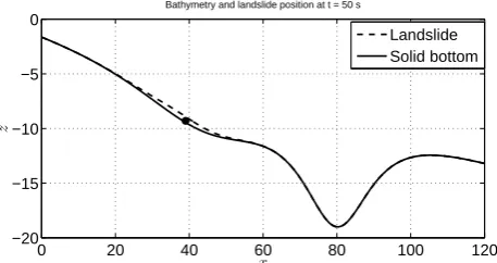
The main aim of the current work is to study the dispersive wave generation in a closed basin (Beisel et al., 2012) using a more realistic landslide model (Chubarov et al., 2005) while keeping the simplicity of the shallow-water approach. To this end, we use the so-called Peregrine system, which is a partic-ular case of a general class of model systems that arise in the Boussinesq scaling (Boussinesq, 1871). A common feature of all Boussinesq-type systems is that they allow a simplified study of surface waves in which both nonlinear and disper-sive effects are taken into account. In the present case, we need to use a Boussinesq system that can handle complex and time-dependent bottom topography. Such a system was derived by Wu (1987), and can be used in connection with the dynamic bathymetry. An example of the type of situation considered here is shown in Fig. 1, which shows how the bathymetry is given by the combination of a solid bottom, and a landslide profile sliding along the fixed bottom.
We conduct two main experiments. First, a comparison with the shallow-water theory is carried out. Second, the de-pendence of the tsunami characteristics on the initial depth of the landslide is investigated. The main findings of the present work are that the predictions of the shallow-water and Boussinesq theory are divergent for the cases treated in this paper, and that the effect of a finite fluid domain, such as a river, lake or fjord (Poncet et al., 2010), can lead to signif-icantly different behavior when compared to tsunamis on an open ocean (see also Beisel et al., 2012).
The Boussinesq model in this paper is based on the as-sumption of an inviscid fluid, and irrotational flow. These are standard assumptions in the study of surface waves, and
Boussinesq modeling of underwater landslides 3 /33
0 20 40 60 80 100 120
−20 −15 −10 −5 0
x
z
Bathymetry and landslide position at t = 50 s
Landslide Solid bottom
Figure 1. The fixed bathymetryz=h0(x)and the position of the landslide after
50s. The position of the barycenter is indicated by a black dot.
is only approximate, and in particular, one important effect of surface waves, namely the influence of frequency dispersion is neglected.
The main aim of the current work is to study the dispersive wave generation in a closed
basin [7] using a more realistic landslide model [15] while keeping the simplicity of the
shallow-water approach. To this end, we use the so-called Peregrine system which is a particular case of a general class of model systems which arise in the Boussinesq scaling
[12]. A common feature of all Boussinesq-type systems is that they allow a simplified study
of surface waves in which both nonlinear and dispersive effects are taken into account. In the present case, we need to use a Boussinesq system which can handle complex and
time-dependent bottom topography. Such a system was derived by Wu [67], and can be used in
connection with the dynamic bathymetry. An example of the type of situation considered
here is shown in Figure1, which shows how the bathymetry is given by the combination
of a solid bottom, and a landslide profile sliding along the fixed bottom.
We conduct two main experiments. First, a comparison with the shallow-water theory is carried out. Second, the dependence of the tsunami characteristics on the initial depth of the landslide is investigated. The main findings of the present work are that the predictions of the shallow-water and Boussinesq theory are divergent for the cases treated in this paper, and that the effect of a finite fluid domain, such as a river, lake or fjord [51] can lead to significantly different behavior when compared to tsunamis on an open ocean (see also
[7]). The Boussinesq model in this paper is based on the assumption of an inviscid fluid,
and irrotational flow. These are standard assumptions in the study of surface waves, and generally give good results, unless there are strong background currents in the fluid. Another effect which is not taken account of here is the wave resistance on the landslide due
to waves created by the motion of the landslide. However, as observed in [39], this effect
is negligible for most realistic cases of underwater landslides. Viscosityisincluded in the
dynamic model for the landslide as will be shown in the next section. In order to capture the effect of slide deformation during the evolution, a damping term in the equation of motion is included to model the internal friction in the landslide mass.
Fig. 1. The fixed bathymetryz=h0(x)and the position of the
land-slide after 50 s. The position of the barycenter is indicated by a black dot.
generally give good results, unless there are strong back-ground currents in the fluid. Another effect that is not taken account of here is the wave resistance on the landslide due to waves created by the motion of the landslide. However, as observed in Harbitz et al. (2006), this effect is negligible for most realistic cases of underwater landslides. Viscosity
is included in the dynamic model for the landslide as will
be shown in the next section. In order to capture the effect of slide deformation during the evolution, a damping term in the equation of motion is included to model the internal friction in the landslide mass.
The paper is organized in the following way. In Sect. 2, the equation of motion for the landslide is developed. Then in Sect. 3, the Boussinesq model is recalled. In Sect. 4, solitary-wave solutions of the Peregrine system are found numeri-cally. In Sect. 5, the numerical scheme for the Boussinesq system is explained and the numerical method is tested using the exact solutions of Sect. 4. Section 6 contains results of nu-merical runs for a few specific cases of bottom bathymetry, a parameter study of wave run-up in relation to the initial depth of the landslide, and a comparison with the shallow-water theory.
2 The landslide model
In this section we briefly present a mathematical model of un-derwater landslide motion. This process has to be addressed carefully since it determines the subsequent formation of wa-ter waves at the free surface. In the present study, we will assume the movable mass to be a solid body with a pre-scribed shape and known physical properties. Since the land-slide mass and volume is preserved during the evolution, it is sufficient to determine the position of the barycenter
x=xc(t )as a proxy for the motion of the whole body. As
observed in the introduction, most studies of wave generation due to underwater landslides are based on prescribed bottom
motion, or on solving the equation of motion on a uniform
D. Dutykh and H. Kalisch: Boussinesq modeling of underwater landslides 269
viscous terms. Examples of such works include the follow-ing: DiRisio et al. (2009); Pelinovsky and Poplavsky (1996); Watts et al. (2000). A more general approach was recently pioneered by Khakimzyanov and Shokina (2010), where cur-vature effects of the bottom topography were taken into ac-count. Since this model is applicable to a wider range of cases, we follow the approach of Khakimzyanov and Shok-ina (2010). However, in addition to the effects included by Khakimzyanov and Shokina, our model also incorporates the effect of internal friction in the slide material (given by the dissipative forceFi) and the action of bottom friction, given
byFb.
The static bathymetry is prescribed by a sufficiently smooth single-valued function z= −h0(x), and the
land-slide shape is initially prescribed by a localized function
z=ζ0(x). To be specific, in this study we choose the
fol-lowing shape function for the landslide mass:
ζ0(x)=A
(
1 2
1+cos(2π(x−x0)
` )
, |x−x0| ≤`2
0, |x−x0|>2`.
(1)
In this formula,Ais the maximum height,`the length of the slide andx0the initial position of its barycenter. It is clear
that the model description given below and the method of nu-merical integration used in the present work is applicable to any other smooth profile, as long as it is sufficiently localized and fully submerged.
Since the landslide motion is translational, its shape at time
tis given by the functionz=ζ (x, t )=ζ0(x−xc(t )). Recall
that the landslide center is located at a point with abscissa
x=xc(t ). Then, the impermeable bottom for the water wave
problem can be easily determined at any time by simply su-perposing the static and dynamic components. Thus the bot-tom boundary conditions for the fluid are to be imposed at
z= −h(x, t )= −h0(x)+ζ (x, t ).
To simplify the subsequent presentation, we introduce the classical arc-length parameterization, where the parameter
s=s(x)is given by the formula
s=L(x)= x
Z
x0 q
1+(h00(ξ ))2dξ. (2)
The functionL(x)is monotone and can be efficiently in-verted to yield the original Cartesian abscissax=L−1(s). Within the parameterization in Eq. (2), the center of the land-slide is initially located at a point with the curvilinear coor-dinates=0. The local tangential direction is denoted byτ
and the normal direction byn.
A straightforward application of Newton’s second law re-veals that the landslide motion is governed by the differential equation
md
2s
dt2 =Fτ(t ),
wherem is the landslide mass and Fτ(t )is the tangential
component of the sum of forces acting on the moving sub-merged body. In order to project the forces onto the axes of the local coordinate system, the angleθ (x)betweenτ and
Oxis needed. This angle is determined by
θ (x)= −arctan h00(x) .
Let us denote byρwandρ`the densities of the water and
landslide material correspondingly. IfV is the volume of the slide, then the total massmis given by the expression
m= ρ`+cwρwV , (3)
where cw is the added mass coefficient. As explained in
Batchelor (2000), a portion of the water mass has to be added to the mass of the landslide since it is entrained by the under-water body motion. For a cylinder, the coefficientcwis equal
exactly to one, but in the present case, the coefficient has to be estimated. The volume of the sliding material is given by
V =W·S, whereW is the landslide width in the transverse direction, andScan be computed by
S=
Z
R
ζ0(x)dx.
The last integral can be computed exactly for the particular choice in Eq. (1) of the landslide shape to give
V =1
2`AW.
The total projected force acting on the landslide can be conventionally represented as a sum of the force Fg
repre-senting the joint action of gravity and buoyancy, and the total contribution of various dissipative forces.
The gravity and buoyancy forces act in opposite directions, and their horizontal projectionFgcan be easily computed by
Fg(t )=(ρ`−ρw)W g
Z
R
ζ (x, t )sin θ (x)dx.
Now, let us specify the dissipative forces. The water resis-tance to the motion of the landslide Fr due to viscous
dis-sipation is proportional to the maximal transverse section of the moving body and to the square of its velocity. In addition, the coefficient sign ddst
is needed to dissipate the landslide kinetic energy independently of its direction of motion. Thus the forceFrtakes the form
Fr= −sign
ds
dt 1
2cdρwAW
ds
dt 2
,
wherecdis the resistance coefficient of the water. The
fric-tion forceFfis proportional to the normal force exerted on
the body due to the weight:
Ff= −cfsign
ds
dt
N (x, t ).
270 D. Dutykh and H. Kalisch: Boussinesq modeling of underwater landslides
The normal forceN (x, t )is composed not only of the normal components of gravity and buoyancy forces, but also of the centripetal force due to the variation of the bottom slope:
N (x, t )=(ρ`−ρw)gW
Z
R
ζ (x, t )cosθ (x)
dx
+ρ`W
Z
R
ζ (x, t )κ(x)ds
dt 2
dx.
Hereκ(x)is the signed curvature of the bottom, which can be computed using the formula
κ(x)= h
00
0(x)
1+(h00(x))232 .
We note that the last term vanishes for a plane bottom since
κ(x)≡0 in this particular case. Energy loss inside the sliding material due to internal friction is modeled by
Fi= −cvρ`W S
ds
dt,
wherecvis an internal friction coefficient. Finally,
dissipa-tion in the boundary layer between the landslide and the solid bottom is taken account of by the term
Fb= −cbρwW `
ds
dt
ds
dt ,
wherecbis the Ch´ezy coefficient.
Finally, if we sum up the contributions of all the forces de-scribed above, we obtain the second-order differential equa-tion
(γ+cw)S
d2s
dt2 =(γ−1)g
I1(t )−cfσ (t )I2(t )
−σ (t )cfγI3(t )+
1 2cdA
ds
dt 2
−cvγ S
ds
dt −cb`
ds
dt
ds
dt
, (4)
whereγ = ρ`
ρw >1 is the ratio of densities,σ (t )=sign
ds
dt
and the integralsI1,2,3(t )are defined by
I1(t )=
Z
R
ζ (x, t )sin θ (x)
dx,
I2(t )=
Z
R
ζ (x, t )cos θ (x)
dx,
I3(t )=
Z
R
ζ (x, t )κ(x)dx.
In order to obtain a well-posed initial value problem, Eq. (4) has to be supplemented with initial conditions for
D. Dutykh & H. Kalisch 6 /33
0 50 100 150 200 250 0
50 100 150
t
xc
(
t)
Landslide trajectory tan(1°)
tan(2°)
tan(3°)
0 50 100 150 200 250 −2
−1 0 1 2
t
vc
(
t)
Landslide speed
tan(1°) tan(2°) tan(3°)
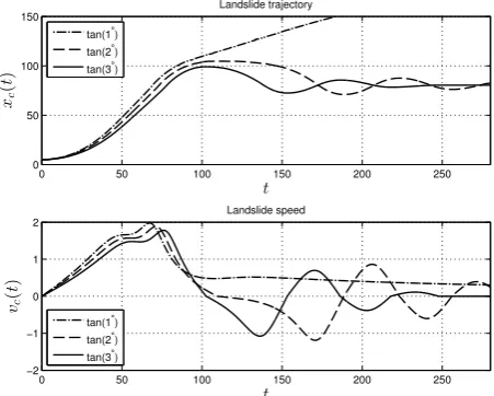
Figure 2. Position and velocity of the barycenter of the landslide as functions of dimensional time for three different values of the friction coefficient
cf.
is needed to dissipate the landslide kinetic energy independently of its direction of motion.
Thus the forceFrtakes the form
Fr=−sign
ds
dt 1
2cdρwAW ds
dt 2
,
wherecdis the resistance coefficient of the water. The friction forceFf is proportional to
the normal force exerted on the body due to the weight:
Ff=−cfsign
ds dt
N(x, t).
The normal forceN(x, t) is composed of the normal components of gravity and buoyancy
forces, but also of the centripetal force due to the variation of the bottom slope:
N(x, t) = (ρℓ−ρw)gW
Z
R
ζ(x, t) cos θ(x)
dx+ρℓW
Z
R
ζ(x, t)κ(x)ds
dt 2
dx.
Hereκ(x) is the signed curvature of the bottom which can be computed using the formula
κ(x) = h
′′
0(x)
1 + (h′
0(x))2
32
.
We note that the last term vanishes for a plane bottom sinceκ(x)≡0 in this particular
case. Energy loss inside the sliding material due to internal friction is modeled by
Fi=−cvρℓW S
ds dt,
Fig. 2. Position and velocity of the barycenter of the landslide as
functions of dimensional time for three different values of the fric-tion coefficientcf.
s(0)and s0(0). In the remainder we always take homoge-neous initial conditions, and consider the motion driven only by the gravitational acceleration of the landslide. However, different boundary conditions might also be reasonable from a modeling point of view.
In order to approximate solutions of Eq. (4), we employ the Bogacki–Shampine third-order Runge–Kutta scheme. The integrals I1,2,3(t ) are computed using the trapezoidal
rule, and once the landslide trajectorys=s(t )is found, we use Eq. (2) to find its motionx=xc(t )in the initial Cartesian
coordinate system. This yields the bottom motion that drives the fluid solver.
For illustrative purposes we show a few examples of land-slide trajectories over the bottom profile depicted in Fig. 1. The other parameters used in the simulations are given in Sect. 6 and also in Table 2. We performed a series of sim-ulations in order to study the effect of various dissipative terms on the landslide trajectory. The dependence on the fric-tion coefficient cf is shown in Fig. 2 where the landslide
barycenter position xc(t ) and its velocity vc(t ) are shown
as functions of time for cf=tan(1◦), tan(2◦) and tan(3◦).
In the case of the weak frictioncf=tan(1◦), the landslide
reaches a sufficient speed to escape from the basin depicted in Fig. 1. For the latter case (cf=tan(3◦)), we show also
si-multaneously the landslide speedvc(t )=ddxtc and its
acceler-ationac(t )=ddvtc =d
2x c
dt2 in Fig. 3. In particular, one can see
that the acceleration is a discontinuous function whose jumps correspond exactly to moments of time where the speedvc
changes its sign, in accordance with the employed model in Eq. (4). However, in our model there are also two new dissi-pative termsFi andFbwhose importance has to be studied
also. We fix the value ofcf=tan(3◦)for all subsequent
D. Dutykh and H. Kalisch: Boussinesq modeling of underwater landslides 271
Boussinesq modeling of underwater landslides 7 /33
0 50 100 150 200 250
−2 −1 0 1 2 t vc ( t ) Landslide speed
0 50 100 150 200 250
−0.1 −0.05 0 0.05 0.1 t ac ( t ) Landslide acceleration
Figure 3. Velocity and acceleration of the barycenter of the landslide as a func-tion of dimensional time. The fricfunc-tion coefficient iscf = tan(3◦). The
discontinuities in the acceleration are due to the coefficientsign ddst
in the definition of the friction force.
wherecv is an internal friction coefficient. Finally, dissipation in the boundary layer
be-tween the landslide and the solid bottom is taken account of by the term
Fb=−cbρwW ℓ
ds dt ds dt ,
wherecbis the Ch´ezy coefficient.
Finally, if we sum up the contributions of all the forces described above, we obtain the second order differential equation
(γ+cw)S
d2s
dt2 = (γ−1)g
I1(t)−cfσ(t)I2(t)
−σ(t)cfγI3(t) + 1 2cdA
ds
dt 2
−cvγS
ds dt−cbℓ
ds dt ds dt , (2.4)
whereγ:= ρℓ
ρw >1 is the ratio of densities,σ(t) := sign
ds
dt
and the integralsI1,2,3(t) are defined by
I1(t) =
Z
R
ζ(x, t) sin θ(x)
dx,
I2(t) =
Z
R
ζ(x, t) cos θ(x)
dx,
I3(t) =
Z
R
ζ(x, t)κ(x) dx.
Fig. 3. Velocity and acceleration of the barycenter of the
land-slide as a function of dimensional time. The friction coefficient is
cf=tan(3◦). The discontinuities in the acceleration are due to the
coefficient sign ddstin the definition of the friction force.
D. Dutykh & H. Kalisch 8 /33
0 50 100 150 200 250 0 20 40 60 80 100 t xc ( t ) Landslide trajectory c
v = 5× 10
−3
c
v = 5× 10
−2
cv = 7.5× 10⁻²
0 50 100 150 200 250 −2 −1 0 1 2 t vc ( t ) Landslide speed c
v = 5× 10
−3
c
v = 5× 10
−2
c
v = 7.5× 10 −2
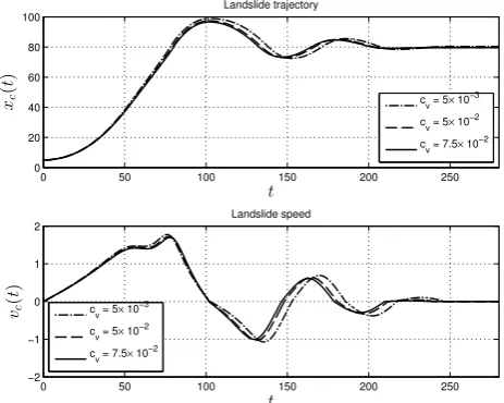
Figure 4. Position and velocity of the barycenter of the landslide as functions of dimensional time for three different values of the friction coefficient
cv.
In order to obtain a well-posed initial value problem, equation (2.4) has to be supplemented with initial conditions fors(0) and s′
(0). In the remainder we always take homogeneous initial conditions, and consider the motion driven only by the gravitational acceleration of the landslide. However, different boundary conditions might also be reasonable from a modeling point of view.
In order to approximate solutions of equation (2.4), we employ the Bogacki-Shampine third-order Runge-Kutta scheme. The integralsI1,2,3(t) are computed using the trapezoidal
rule, and once the landslide trajectorys=s(t) is found, we use equation (2.2) to find its motionx=xc(t) in the initial Cartesian coordinate system. This yields the bottom motion
that drives the fluid solver.
For illustrative purposes we show a few examples of landslide trajectories over the bottom profile depicted in Figure1. The other parameters used in the simulations are given in Section6 and also in Table 2. We performed a series of simulations in order to study the effect of various dissipative terms on the landslide trajectory. The dependence on the friction coefficientcf is shown in Figure 2 where the landslide barycenter position xc(t)
and its velocityvc(t) are shown as functions of time forcf = tan(1◦), tan(2◦) and tan(3◦).
n the case of the weak frictioncf = tan(1
◦
), the landslide reaches a sufficient speed to escape from the basin depicted on Figure1. For the latter case (cf = tan(3◦)) we show
also simultaneously the landslide speedvc(t) :=dxdtx and its accelerationac(t) := dvdtc = d 2
xc dt2
in Figure3. In particular, one can see that the acceleration is a discontinuous function whose jumps correspond exactly to moments of time where the speedvcchanges its sign,
in accordance with the employed model (2.4). However, in our model there are also two new dissipative termsFi and Fb whose importance has to be studied also. We fix the
Fig. 4. Position and velocity of the barycenter of the landslide as
functions of dimensional time for three different values of the fric-tion coefficientcv.
cvandcbfor other fixed parameters given in Table 2. These
numerical results are presented in Figs. 4 and 5. One can see that the influence of these parameters on the landslide tra-jectory is weaker. However, we choose to keep them in the model in order to have more latitude for fine-tuning the slide trajectory if need be.
3 The Boussinesq model
Once the motion of the landslide is determined, and there-fore the time-dependent bathymetryh(x, t )=h0(x)−ζ (x, t )
Boussinesq modeling of underwater landslides 9 /33
0 50 100 150 200 250
0 20 40 60 80 100 t xc ( t ) Landslide trajectory c
b = 1× 10
−3
c
b = 7.5× 10
−3
c
b = 1× 10
−2
0 50 100 150 200 250
−2 −1 0 1 2 t vc ( t ) Landslide speed c
b = 1× 10
−3
c
b = 7.5× 10
−3
c
b = 1× 10
−2
Figure 5. Position and velocity of the barycenter of the landslide as functions of dimensional time for three different values of the friction coefficient
cb.
value ofcf = tan(3◦) for all subsequent experiments and we will vary only the two other
coefficients cv andcb for fixed other parameters given in Table 2. These numerical results
are presented in Figures 4 and 5. One can see that the influence of these parameters on the landslide trajectory is weaker. However, we choose to keep them in the model in order to have more latitude for fine tuning the slide trajectory if need be.
3. The Boussinesq model
Once the motion of the landslide is determined, and therefore the time-dependent bathymetry h(x, t) = h0(x)−ζ(x, t) is given, the next step is to consider the coupling
between the bathymetry variations and the evolution of surface waves. The main assump-tions on the fluid are that it is inviscid and incompressible, and that the flow is irrotational. Under these assumptions, the potential-flow free surface problem governs the motion of the fluid. However, in the present case, the fluid is shallow, and the waves at the surface are of small amplitude when compared to the depth of the fluid. In that case, the potential-flow problem may be simplified, and the model used in this paper is a variant of the so-called classical Boussinesq system derived by Boussinesq [12].
Let us first consider the case of an even bottom, and a constant fluid depthd0. Denote
a typical wave amplitude by a, and a typical wavelength by λ. The parameter α = a d0
then describes the relative amplitude of the waves, and the parameter β = d20
λ2 measures
the ’shallowness’ of the fluid in comparison to the wavelength. In the case when bothα
Fig. 5. Position and velocity of the barycenter of the landslide as
functions of dimensional time for three different values of the fric-tion coefficientcb.
is given, the next step is to consider the coupling between the bathymetry variations and the evolution of surface waves. The main assumptions on the fluid are that it is inviscid and incompressible, and that the flow is irrotational. Under these assumptions, the potential-flow free surface problem governs the motion of the fluid. However, in the present case, the fluid is shallow, and the waves at the surface are of small amplitude when compared to the depth of the fluid. In that case, the potential-flow problem may be simplified, and the model used in this paper is a variant of the so-called classical Boussinesq system derived by Boussinesq (1871).
Let us first consider the case of an even bottom, and a con-stant fluid depthd0. Denote a typical wave amplitude bya,
and a typical wavelength byλ. The parameterα= a d0 then
describes the relative amplitude of the waves, and the param-eterβ=d
2 0
λ2 measures the “shallowness” of the fluid in
com-parison to the wavelength. In the case when bothαandβare small and approximately of the same order of magnitude, the system
ηt+d0ux+(ηu)x=0,
ut+gηx+uux−
d02
3 uxxt=0
(5)
may be used as an approximate model for the description of the evolution of the surface waves and the fluid flow. In Eq. (5),ηdenotes the deflection of the free surface from its rest position, andudenotes the horizontal fluid velocity at a heightz=d0(−1+
√
1/3)in the fluid column ifzis mea-sured from the rest position of the free surface. The same equation appears if the velocity is taken to be the average of the horizontal velocity over the flow depth.
272 D. Dutykh and H. Kalisch: Boussinesq modeling of underwater landslides
The system in Eq. (5) was first derived by Peregrin (1967), and falls into a general class of Boussinesq systems, as shown in the systematic studies (Bona et al., 2002; Nwogu, 1993). As opposed to the shallow-water approximation, the pressure is not assumed to be hydrostatic, and the horizontal velocity varies with depth. In fact, the horizontal velocity profile is a quadratic function ofz(Whitham, 1974). Non-hydrostatic effects lead to the appearance of linear dispersive terms in the governing equations. The problem of landslide-generated waves has been addressed in the fully nonlinear shallow wa-ter framework (Watts et al., 2003; Chubarov et al., 2005; Yu et al., 2007; Beisel et al., 2010). Nevertheless, several authors have recently obtained interesting results even in the linear (Sammarco and Renzi, 2008; Seo and Liu, 2013) or nonlin-ear (Fernandez-Nieto et al., 2008; Didenkulova et al., 2010; Beisel et al., 2012) hydrostatic models.
The derivation of Eq. (5) given in Peregrin (1967) also featured an extension to non-constant but time-independent bathymetry. However, the present case of a dynamic bot-tom profile calls for a system that allows for time-dependent bathymetry, and such a system was derived in Wu (1987). Given a bottom topography described byz= −h(x, t ), the system takes the form
ηt+ (h+η)ux+ht=0,
ut+gηx+uux=
1
2h ht+(hu)x
xt−
h2
6 uxxt.
(6)
In order for this system to be asymptotically valid, we need
α∼β as before. Moreover, concerning the unsteady bottom profile, we make the assumptions thathx≤O(αβ1/2), and
ht≤O(αβ1/2).
In comparison to the shallow-water equations with a time-dependent bottom topography, the system in Eq. (6) has ad-ditional terms on the right-hand side of the second equation. The effect of these terms is to incorporate frequency disper-sion into the model. One practical aspect of this modifica-tion is that wave breaking can be completely avoided as long as the amplitude of the waves is small enough. Wave break-ing is also possible in evolution systems of Boussinesq type (Bjørkav˚ag and Kalisch, 2011; Briganti et al., 2004), but the amplitudes occurring in the present problem are far from the breaking limit. The phase speed of a small-amplitude linear wave of wavelength 2π/ kin Eq. (6) with a stationary even bottom has the formc2= gd0
1+d
2 0 3k2
,while the phase speed is given byc2=gd0tanhkd(kd0)
0 in the linearized full water wave
problem. Thus one might argue that the dispersion in Eq. (6) is too strong in comparison with dispersion in realistic wa-ter waves. However, as discussed in Bjørkav˚ag and Kalisch (2011), the linear dispersion relation of Eq. (6) is still closer to the dispersion relation of the original water-wave problem than most other standard Boussinesq equations that feature even faster decay of the phase speed with increasingk.
4 Solitary waves
Before the numerical method for approximating solutions of Eq. (6) is presented, we digress for a moment, and ex-plain how to find numerically exact solutions of the system in Eq. (5). These solutions will later be used to test the imple-mentation of the numerical procedure. Assuming the special form
η(x, t )=η(ξ ), u(x, t )=u(ξ ), ξ =x−cst,
and substituting this representation into the governing Eq. (5), the following appears:
−csη0+ (d+η)u
0
=0,
−csu0+
1 2(u
2)0+gη0+c
s
d2
3 u 000 =0.
Assuming decay of both η andu to zero as|x| → ∞, the integration of the mass conservation equation from−∞toξ
gives the following relation betweenηandu:
u= csη
d+η, η= d·u cs−u
. (7)
The momentum balance equation can now be integrated to yield
−cs
u−d
2
3 u 00+1
2u
2+gη=0. (8)
Finally, in order to obtain a closed form equation in terms of the velocity u, we substitute the expression in Eq. (7) forηinto Eq. (8). The resulting differential equation can be written in operator notation as
Lu=N(u),
where the linear operatorLand the nonlinear operatorN are defined respectively by
Lu=cs
u−d
2
3 u
00 and N(u)=1 2u
2+ gdu
cs−u
.
While nothing formal appears to be known about existence of localized solutions of Eqs. (7) and (8), it is straightforward to compute approximations of solitary waves numerically. In particular, one may use the well-known Petviashvili iteration method, which takes the form
un+1=L−1·N(un)·
(u
n,N(un))
(un,Lun)
−q
. (9)
The exponentqis usually defined as a function of the de-greep of the nonlinearity, with the rule of thumb that the expressionq= p
p−1 generally works well. In our case, the
D. Dutykh and H. Kalisch: Boussinesq modeling of underwater landslides 273
D. Dutykh & H. Kalisch
12 /
33
−10 −5 0 5 10
0 0.05 0.1 0.15 0.2 0.25 0.3 0.35 0.4 0.45 0.5
Free surface elevation
x
η
(
x
)
Peregrine system Grimshaw solution
c= 1.05
c= 1.15
c= 1.1
c= 1.2
(a)
−10 −5 0 5 10
0 0.05 0.1 0.15 0.2 0.25
Depth−averaged horizontal velocity
x
u
(
x
)
Peregrine system Grimshaw solution
c= 1.025 c= 1.05 c= 1.1
c= 1.12
(b)
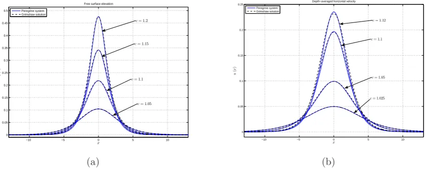
Figure 6.
Comparison of the numerical approximation of solitary wave solutions
of
(
3.1)
to Grimshaw’s third-order asymptotic approximation of
soli-tary waves using the Euler equations for the full water wave problem.
The left panel shows the surface elevation, and the right panel shows
the horizontal velocity at
z
=
d
0(
−
1 +
p
1/3).
The exponent
q
is usually defined as a function of the degree
p
of the nonlinearity, with
the rule of thumb that the expression
q
:=
p−p1generally works well. In our case, the
nonlinearities are quadratic, so that we choose
p
= 2, and hence
q
= 1.
The Petviashvili method was analyzed in [
48
], and can be very efficiently implemented
using the Fast Fourier Transform [
28
]. The iteration can be started for instance with the
third-order asymptotic solution of Grimshaw [
37
]. The iterative procedure is continued
until the
L
∞norm between two successive iteration is on the order of machine precision.
Figure
6
shows approximate solitary-wave solutions of (
3.1
) with various wave speeds, and
compares them to the third-order asymptotic approximation of solitary-wave solutions of
the full water-wave problem obtained by Grimshaw [
37
]. The left panel shows comparisons
of the free-surface excursion, while the right panel shows a comparison of the horizontal
component of the velocity field, evaluated at the non-dimensional height ˜
z
given by ˜
z
=
−
1 +
p
1
/
3. Figure
7
shows a comparison of the wavespeed-amplitude relation between
the solitary-wave approximation of (
3.1
) and the ninth-order asymptotic approximation to
the full water-wave problem obtained by Fenton [
26
].
Fig. 6. Comparison of the numerical approximation of solitary wave solutions of Eq. (5) to Grimshaw’s third-order asymptotic approximation
of solitary waves using the Euler equations for the full water wave problem. The upper panel shows the surface elevation, and the lower panel shows the horizontal velocity atz=d0(−1+
√ 1/3).
The Petviashvili method was analyzed in Stepanyants and Pelinovsky (2004), and can be very efficiently implemented using the fast Fourier transform (FFT) (Frigo and Johnson, 2005). The iteration can be started for instance with the third-order asymptotic solution of Grimshaw (1971). The iterative procedure is continued until theL∞norm between two suc-cessive iteration is on the order of machine precision. Fig-ure 6 shows approximate solitary-wave solutions of Eq. (5) with various wave speeds, and compares them to the third-order asymptotic approximation of solitary-wave solutions of the full water-wave problem obtained by Grimshaw (1971). The left panel shows comparisons of the free-surface ex-cursion, while the right panel shows a comparison of the horizontal component of the velocity field, evaluated at the non-dimensional heightz˜given byz˜= −1+√1/3. Figure 7 shows a comparison of the wave-speed–amplitude relation between the solitary-wave approximation of Eq. (5) and the ninth-order asymptotic approximation to the full water-wave problem obtained by Fenton (1972).
5 The numerical scheme
For the numerical discretization, a finite-volume discretiza-tion procedure similar to the one used in Barth (1994) and Barth and Ohlberger (2004) is employed. Let us take as a unit of length the undisturbed depthd0of the fluid above the
barycenter of the landslide, and as a unit of time the ratio
q
d0
g. Then the Peregrine system in Eq. (6) is rewritten in
terms of the total water depthHas
Boussinesq modeling of underwater landslides 13 /33
0 0.05 0.1 0.15 0.2 0.25 0.3 0.35 1
1.02 1.04 1.06 1.08 1.1 1.12 1.14 1.16
Amplitude − Wave speed diagram
a
0/d
cs
/(gd)
1/2
Fenton solution Classical Peregrine
Figure 7. Amplitude-speed relation of solitary wave solutions of (3.1) and of Fenton’s ninth-order asymptotic approximation of solitary waves us-ing the Euler equations for the full water wave problem.
5. The numerical scheme
For the numerical discretisation, a finite-volume discretisation procedure similar to the one used in [4,5] is employed. Let us take as a unit of length the undisturbed depthd0 of
the fluid above the barycenter of the landslide, and as a unit of time the ratioqd0 g. Then
the Peregrine system (3.2) is rewritten in terms of the total water depthH as
Ht + [Hu]x = 0, (5.1)
ut +
1 2u
2+ (H−h) x =
1 2hhxtt+
1
2h(hu)xxt− 1 6h
2u
xxt, (5.2)
The system (5.1), (5.2) can be formally rewritten in the form
Vt + [F(V) ]x = Sb + M(V), (5.3)
where the densityV and the advective fluxF(V) are defined by
V ≡
H u
, F(V) ≡
H u
1
2u2 + (H−h)
.
The source term is defined by
Sb ≡
0
1 2hhxtt
,
and the dispersive term is defined by
M(V) ≡
0
1
2h(hu)xxt− 1 6h
2u xxt
.
Fig. 7. Amplitude–speed relation of solitary wave solutions of
Eq. (5) and of Fenton’s ninth-order asymptotic approximation of solitary waves using the Euler equations for the full water wave problem.
Ht + [H u]x =0, (10)
ut + 12u2+(H−h)x =
1 2hhxt t+
1
2h(hu)xxt
−1
6h
2u
xxt. (11)
The system in Eqs. (10) and (11) can be formally rewritten in the form
Vt + [F(V)]x = Sb + M(V), (12)
274 D. Dutykh and H. Kalisch: Boussinesq modeling of underwater landslides
where the density V and the advective fluxF(V)are de-fined by
V ≡
H
u
, F(V) ≡
H u
1 2u
2+(H−h)
.
The source term is defined by
Sb ≡
0
1 2hhxt t
,
and the dispersive term is defined by
M(V) ≡
0
1
2h(hu)xxt− 1 6h2uxxt
.
We begin our presentation with a discretization of the hy-perbolic part of Eqs. (10) and (11), which is the classical non-linear shallow-water system, and then discuss the treatment of dispersive terms. The Jacobian of the advective fluxF(V) is easily computed to be
A(V) = ∂F(V)
∂V =
u H
1 u
,
and it is clear thatA(V)has the two distinct eigenvalues
λ± = u ± cs, cs ≡ √
H .
The corresponding right and left eigenvectors are the columns of the matrices
R =
H−H cs cs
, L = R−1 = 1
2
H−1 cs−1
−H−1cs−1
.
We consider a partition of the real line R into cells (or finite volumes)Ci= [xi−1
2, xi+ 1 2
]with cell centersxi= 1
2(xi−1
2
+xi+1 2
)(i∈Z). Let1xidenote the length of the cell
Ci. In the following we will consider only uniform partitions
with1xi = 1x,∀i∈Z. We would like to approximate the solution V(x, t )by discrete values. In order to do so, we in-troduce the cell average of V on the cellCi(denoted with an
overbar):
¯
Vi(t ) ≡ H¯i(t ) ,u¯i(t ) =
1
1x Z
Ci
V(x, t )dx.
A simple integration of Eq. (12) over the cellCi leads to
the exact relation dV¯
dt +
1
1x h
F(V(xi+12, t ))−F(V(xi−12, t ))
i
= 1
1x Z
Ci
Sb(V)dx ≡ ¯Si.
Since the discrete solution is discontinuous at cell inter-facesxi+1
2
(i∈Z), we replace the flux at the cell faces by the so-called numerical flux function
F(V(xi±12, t )) ≈ Fi±12(V¯
L i±1
2 ,V¯R
i±1
2 ),
whereV¯L,R i±1
2
denotes the reconstructions of the conservative variablesV from left and right sides of each cell interface (the¯
reconstruction procedure employed in the present study will be described below). Consequently, the semi-discrete scheme takes the form
dV¯i
dt +
1
1x
Fi+12 −Fi−12
= ¯
Si. (13)
In order to discretize the advective fluxF(V), we follow the method of Ghidaglia et al. (1996, 2001) and use the fol-lowing finite volume characteristic flux (FVCF) scheme:
F(V,W) = F(
V)+F(W)
2 − U(V,W)·
F(W)−F(V)
2 .
The first part of the numerical flux is centered, while the second part is the upwinding introduced through the Jacobian sign-matrixU(V,W)defined by
U(V,W) = signA(12(V+W))
,
sign(A) = R·diag(s+, s−)·L,
wheres±≡sign(λ±). After some simple algebraic compu-tations, one can find
U =
1 2
s++s− (H /cs) (s+−s−)
(cs/H ) (s+−s−) s++s−
,
the sign-matrixUbeing evaluated at the average state of left and right values.
Finally, the source term Sb(x, t )=(0,12hhxt t), which is
due to the moving bottom, is discretized by evaluating the bathymetry function and its derivatives at cell centers:
1
1x Z
Ci
Sb(x, t )dx≈ 0,21h(xi, t ) hxt t(xi, t ).
Recall that the bathymetry is composed of the static part and of the landslide subject to a translational motion:
h(x, t )=h0(x)−ζ (x, t )=h0(x)−ζ0 x−xc(t ).
The derivativehxt t can be readily obtained from the
for-mula
hxt t(x, t )=
d2xc
dt2
d2ζ0
dx2(x−xc(t ))−
dxc
dt 2d3ζ0
D. Dutykh and H. Kalisch: Boussinesq modeling of underwater landslides 275
5.1 High-order reconstruction
In order to obtain a higher order scheme in space, we need to replace the piecewise constant data by a piecewise poly-nomial representation. This goal is achieved by various so-called reconstruction procedures such as MUSCL TVD (Kol-gan, 1975; van Leer, 1979, 2006), UNO (Harten and Osher, 1987), ENO (Harten, 1989), WENO (Xing and Shu, 2005) and many others. In recent studies on unidirectional wave models (Dutykh et al., 2013a) and on Boussinesq-type equa-tions (Dutykh et al., 2011b), the UNO2 scheme showed a good performance with small dissipation in realistic propa-gation and run-up simulations. Consequently, we retain this scheme for the discretization of the advective flux of the Peregrine system in Eqs. (10) and (11).
The main idea of the UNO2 scheme is to construct a non-oscillatory piecewise-parabolic interpolant Q(x)to a piece-wise smooth function V(x)(see Harten and Osher, 1987, for more details). On each segment containing the facexi+1
2
∈
[xi, xi+1], the function Q(x)=qi+12(x)is locally a quadratic polynomial and whereverv(x)is smooth we have
Q(x) − V(x) = 0 + O(1x3),
dQ
dx(x±0) −
dV
dx = 0 + O(1x
2).
Also, Q(x)should be non-oscillatory in the sense that the number of its local extrema does not exceed that of V(x). Since qi+1
2(xi)
= ¯Viand qi+1
2(xi+1)
= ¯Vi+1, it can be
writ-ten in the form
qi+1 2(x)
= ¯Vi+
di+1 2
{V} ×x−xi
1x +
1
2Di+12{V} ×
(x−xi)(x−xi+1)
1x2 ,
wheredi+1 2
{V} ≡ ¯Vi+1− ¯Vi andDi+1
2V is closely related
to the second derivative of the interpolant sinceDi+1 2
{V} =
1x2q00 i+1
2
(x). The polynomial qi+1
2(x) is chosen to be
the least oscillatory between two candidates interpolat-ing V(x) at (xi−1, xi, xi+1) and (xi, xi+1, xi+2). This
re-quirement leads to the following choice of Di+1 2
{V} ≡
minmod Di{V},Di+1{V}with Di{V} = ¯Vi+1 − 2V¯i + ¯Vi−1, Di+1{V} = ¯Vi+2 − 2V¯i+1 + ¯Vi,
and where minmod(x, y)is the usual minmod function de-fined as
minmod(x, y) ≡ 1
2[sign(x)+sign(y)] ×min(|x|,|y|).
To achieve the second orderO(1x2)accuracy, it is suf-ficient to consider piecewise linear reconstructions in each
cell. LetL(x)denote this approximately reconstructed func-tion, which can be written in the form
L(x) = ¯Vi + Si·
x−xi
1x , x∈ [xi−12, xi+12
].
In order forL(x)to be a non-oscillatory approximation, we use the parabolic interpolation Q(x)constructed below to estimate the slopes Siwithin each cell:
Si = 1x×minmod
dQ
dx(xi−0),
dQ dx(xi+0)
.
In other words, the solution is reconstructed on the cells while the solution gradient is estimated on the dual mesh as it is often performed in more modern schemes (Barth, 1994; Barth and Ohlberger, 2004). A brief summary of the UNO2 reconstruction can be also found in Dutykh et al. (2011b, 2013a).
5.2 Treatment of the dispersive terms
In this section, we explain how to treat the relevant disper-sive terms in the second Eq. (11) of the Peregrine system nu-merically. We propose the following approximation for the second component ofM(V¯)ofM(V¯):
Mi(V¯)=
1 2
¯
hi ¯
hi+1(u¯t)i+1−2h¯i(u¯t)i+ ¯hi−1(u¯t)i−1
1x2
−1
6
¯
hi2(u¯t)i+1−2(u¯t)i+(u¯t)i−1 1x2
= ¯
hi
21x2
¯
hi−1−
1 3
¯
hi
(u¯t)i−1
− 2
31x2 ¯
h2i(u¯t)i+ ¯
hi
21x2
¯
hi+1−
1 3
¯
hi
(u¯t)i+1.
Note that this spatial discretization is of the second order O(1x2)so as to be consistent with the UNO2 advective flux discretization presented above. If we denote byIthe identity matrix, we can now rewrite the semi-discrete scheme in the form
dH¯
dt +
1
1x
F(+1)(V¯)−F
(1)
− (V¯)
= 0, (I−M)·du¯
dt +
1
1x
F(+2)(V¯)−F
(2)
− (V¯)
= S(2)
b ,
whereF(±1,2)(V¯)are the two components of the advective nu-merical flux vectorFat the right (+) and left (−) faces corre-spondingly, andS(b2)denotes the discretization of the second component ofSb.
In order to advance the numerical solution forward in time, one has to invert the matrix(I−M)at every time step. This is no problem in practice, since the matrix appears to be well conditioned in all cases we have considered. In fact, the in-vertibility of the matrix(I−M)can be rigorously shown to hold for small enough 1x since the matrix is then diago-nally dominant. The criterion for diagonal dominance in the
276 D. Dutykh and H. Kalisch: Boussinesq modeling of underwater landslides
present case is seen to be
1+ 2
31x2 ¯
h2i >
−1
6
¯
h2i 1x2+
¯
hi
21x2 ¯
hi−1
+
−1
6
¯
h2i 1x2+
¯
hi
21x2 ¯
hi+1
.
Using a Taylor expansion to express the termsh¯i−1 and ¯
hi+1 as h¯i−1= ¯hi−1xh¯0(xi)+O(1x2) and h¯i+1= ¯hi+
1xh¯0(xi)+O(1x2) , respectively, the criterion reduces to
1+ 1 31x2h¯2i >
¯
hih¯0i
1x +O(1),and this is guaranteed to hold for
small enough1x.
5.3 Time stepping
We assume that the linear system of equations is already in-verted, and we have the following system of ordinary differ-ential equations:
Vt=N(V, t ), V(0)=V0.
In order to solve numerically the last system of equations, we apply the Bogacki–Shampine method proposed by Prze-myslaw Bogacki and Lawrence F. Shampine in 1989 (Bo-gacki and Shampine, 1989). It is a Runge–Kutta scheme of the third order with four stages. It has an embedded second-order method that is used to estimate the local error and thus, to adapt the time step size. Moreover, the Bogacki–Shampine method enjoys the first same as last (FSAL) property so that it needs approximately three function evaluations per step. This method is also implemented in theode23function in MATLAB (Shampine and Reichelt, 1997). The one step of the Bogacki–Shampine method is given by
k1=N(V(n), tn),
k2=N(V(n)+121tnk1, tn+121t ),
k3=N(V(n))+431tnk2, tn+341t ), V(n+1) =V(n)+1tn 29k1+13k2+49k3,
k4=N(V(n+1), tn+1tn),
V(n2+1) =V(n)+1tn 244k1+14k2+13k3+18k4.
Here V(n)≈V(tn), 1t is the time step and V(n2+1) is a
second-order approximation to the solution V(tn+1), so the
difference between V(n+1)and V(n2+1)gives an estimation of the local error. The FSAL property consists in the fact thatk4
is equal tok1in the next time step, thus saving one function
evaluation.
If the new time step 1tn+1 is given by 1tn+1=
ρn1tn, then, according to the H211b digital filter approach
(S¨oderlind, 2003; S¨oderlind and Wang, 2006), the propor-tionality factorρnis given by
ρn=
δ n
β1 δ n−1
β2
ρn−−α1, (14)
wheren is a local error estimation at time steptn, and the
constantsβ1,β2andαare defined by
α=1
4, β1= 1
4p, β2=
1 4p.
The parameterpgives the order of the scheme, andp=3 in our case.
The adaptive strategy in Eq. (14) can be further improved if we smooth the factorρn before computing the next time
step1tn+1:
1tn+1= ˆρn1tn, ρˆn=ω(ρn).
The function ω(ρ) is called the time step limiter and should be smooth, monotonically increasing and should sat-isfy the following conditions:
ω(0) <1, ω(+∞) >1, ω(1)=1, ω0(1)=1.
One possible choice was suggested in S¨oderlind and Wang (2006):
ω(ρ)=1+κarctanρ−1
κ
.
In our computations the parameterκ is set to 1.
5.4 Validation
The scheme described in this section is implemented in MAT-LAB, and runs on a workstation. To check whether the imple-mentation is correct, we use the approximate solitary waves of Eq. (5), computed in the last section. These are used as initial data in the fully discrete scheme, and integrated for-ward in time. The computed solutions are then compared to the same solitary waves, but shifted forward in space byct0,
wherecis the wave speed, andt0is the final time. This
proce-dure is repeated a number of times with different spatial grid sizes. As a result, it is possible to find the spatial convergence rate of the scheme. As is visible in Fig. 8, the convergence achieved by the practical implementation of the discretiza-tion is very close to the theoretical convergence rate. Since the temporal discretization is adaptive, we do not present a convergence study in terms of the timestep1t.
5.4.1 Wave generation by moving bottom
D. Dutykh and H. Kalisch: Boussinesq modeling of underwater landslides 277
D. Dutykh & H. Kalisch
18 /
33
10−1 100
10−5
10−4
10−3
10−2
10−1
100
∆x
ε
Convergence rate inL∞norm
FV scheme, slope = 1.995 2nd order
(a)
10−1 100
10−5
10−4
10−3
10−2
10−1
100
∆x
ε
Convergence rate inL2norm
FV scheme, slope = 2.446 2nd order
(b)
Figure 8.
Convergence rate of the finite-volume scheme in the
L
∞-norm (left
panel) and the
L
2-norm (right panel). The numerical integration of a
solitary wave as shown in Figure
6
is compared to a translated profile.
It appears that the second-order convergence is achieved.
Remark 1.
The adaptive strategy
(
5.5
)
can be further improved if we smooth the factor
ρ
nbefore computing the next time step
∆
t
n+1:
∆
t
n+1= ˆ
ρ
n∆
t
n,
ρ
ˆ
n=
ω
(
ρ
n)
.
The function
ω
(
ρ
)
is called
the time step limiter
and should be smooth, monotonically
increasing and should satisfy the following conditions:
ω
(0)
<
1
,
ω
(+
∞
)
>
1
,
ω
(1) = 1
, ω
′(1) = 1
.
One possible choice was suggested in
[
58
]
:
ω
(
ρ
) = 1 +
κ
arctan
ρ
−
1
κ
.
In our computations the parameter
κ
is set to 1.
5.4. Validation
The scheme described in this section is implemented in MATLAB, and runs on a
work-station. To check whether the implementation is correct, we use the approximate solitary
waves of (
3.1
), computed in the last section. These are used as initial data in the fully
discrete scheme, and integrated forward in time. The computed solutions are then
com-pared to the same solitary waves, but shifted forward in space by
ct
0, where
c
is the wave
speed, and
t
0is the final time. This procedure is repeated a number of times with
differ-ent spatial gridsizes. As a result, it is possible to find the spatial convergence rate of the
scheme. As is visible in Figure
8
, the convergence achieved by the practical implementation
of the discretisation is very close to the theoretical convergence rate. Since the temporal
Fig. 8. Convergence rate of the finite-volume scheme in theL∞-norm (left panel) and theL2-norm (right panel). The numerical integration of a solitary wave as shown in Fig. 6 is compared to a translated profile. It appears that the second-order convergence is achieved.
We consider the linearized water wave problem for a fluid layer of uniform depth z= −d0=const. However, a
por-tion of the bottom can move vertically, and the bottom de-formation is given by a smooth function ζ (x, t ), such that
ζ (x,0)=0. At any given timet, the bottom profile is given byz= −d0+ζ (x, t ). Moreover, we will make a special
as-sumption about the structure of the bottom deformation:
ζ (x, t )=T (t )ζ0(x), T (t )=1−e−αt, α >0, t≥0.
Obviously, we have to assume that||ζ0|| 1 so that the
linear approximation be valid. Then, the free surface eleva-tion at any time is given by the following formula (Hammack, 1973; Dutykh et al., 2006):
η(x, t )= −α 2
2π Z
R
ˆ
ζ0(k)
cosh(kd0) ×
e−αt−cos(ωt )−ω αsin(ωt )
α2+ω2 ·e
−ikxdk, (15)
where ζˆ0(k) is the Fourier transform of ζ0(x) and ω= √
gktanh(kd0)is the wave frequency corresponding to the
wavenumberk. The above integral can be easily computed using the FFT algorithm. To fix the ideas for numerical com-putations, we will take the following localized oscillatory bottom deformation:
ζ0(x)=acos(k0x)e−λ0x
2
, λ0>0.
The values of all parameters used in numerical simula-tion are given in Table 1. The nonlinearity parametera/d0
is chosen to be 0.05, which is far above the nonlinearity of the earthquake-generated tsunamis. However, we think that this value corresponds better to the scope of the present
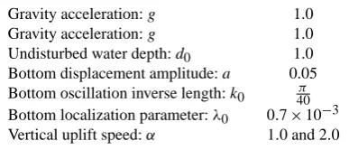
Table 1. Values of various parameters used to simulate the wave
generation by moving bottom.
Gravity acceleration:g 1.0 Gravity acceleration:g 1.0 Undisturbed water depth:d0 1.0
Bottom displacement amplitude:a 0.05 Bottom oscillation inverse length:k0 40π
Bottom localization parameter:λ0 0.7×10⁻³
Vertical uplift speed:α 1.0 and 2.0
study. In order to simulate this setup using the Peregrine sys-tem, we consider a symmetric 1-D computational domain
[−220,220] discretized into N=2000 equal control vol-umes. The time stepping tolerance parameter was set far be-low the spatial discretization error (∼O(1x2)). First, we will take a moderately fast bottom uplift corresponding to the parameterα=1.0. Computational results are presented in Fig. 9a–e. One can see that the overall agreement is fairly good even if some small differences can be noticed in Fig. 9c–d. However, the resulting wave form predicted by the Peregrine system follows closely the linearized full Euler solution in Eq. (15). Now, we will double the bottom uplift speed (α=2.0). This result is presented in Fig. 10a–e. One can see more substantial differences during the generation phase (see panels b–d). However, here again the resulting wave is surprisingly well represented by the Boussinesq-type equations. The observed discrepancies during the generation phase are essentially due to the simplified structure of the vertical speed in Boussinesq-type equations (Dutykh et al., 2013b).
278 D. Dutykh and H. Kalisch: Boussinesq modeling of underwater landslides
Boussinesq modeling of underwater landslides 21 /33
−200 −150 −100 −50 0 50 100 150 200 −0.05
0 0.05
x
η
(
x
,
t
)
Peregrine Cauchy−Poisson
(a)t= 1.5
−200 −150 −100 −50 0 50 100 150 200 −0.05
0 0.05
x
η
(
x
,
t
)
Peregrine Cauchy−Poisson
(b)t= 4.0
−200 −150 −100 −50 0 50 100 150 200 −0.05
0 0.05
x
η
(
x
,
t
)
Peregrine Cauchy−Poisson
(c)t= 8.0
−200 −150 −100 −50 0 50 100 150 200 −0.05
0 0.05
x
η
(
x
,
t
)
Peregrine Cauchy−Poisson
(d)t= 20.0
−200 −150 −100 −50 0 50 100 150 200 −0.05
0 0.05
x
η
(
x
,
t
)
Peregrine Cauchy−Poisson
(e)t= 80.0
Figure 9. Free surface waves generated by a moderately fast bottom motion. The
blue dashed line corresponds to the analytical Cauchy–Poisson solu-tion, while the solid black line is our numerical solution to the Pere-grine system.
Fig. 9. Free surface waves generated by a moderately fast bottom
motion. The blue dashed line corresponds to the analytical Cauchy– Poisson solution, while the solid black line is our numerical solution to the Peregrine system. The time snapshots are taken att=1.5,
t=4,t=8,t=20, andt=80, from top to bottom.
D. Dutykh & H. Kalisch 22 /33
−200 −150 −100 −50 0 50 100 150 200 −0.05
0 0.05
x
η
(
x
,
t
)
Peregrine Cauchy−Poisson
(a)t= 2.5
−200 −150 −100 −50 0 50 100 150 200 −0.05
0 0.05
x
η
(
x
,
t
)
Peregrine Cauchy−Poisson
(b)t= 8.0
−200 −150 −100 −50 0 50 100 150 200 −0.05
0 0.05
x
η
(
x
,
t
)
Peregrine Cauchy−Poisson
(c)t= 15.0
−200 −150 −100 −50 0 50 100 150 200 −0.05
0 0.05
x
η
(
x
,
t
)
Peregrine Cauchy−Poisson
(d)t= 25.0
−200 −150 −100 −50 0 50 100 150 200 −0.05
0 0.05
x
η
(
x
,
t
)
Peregrine Cauchy−Poisson
(e)t= 70.0
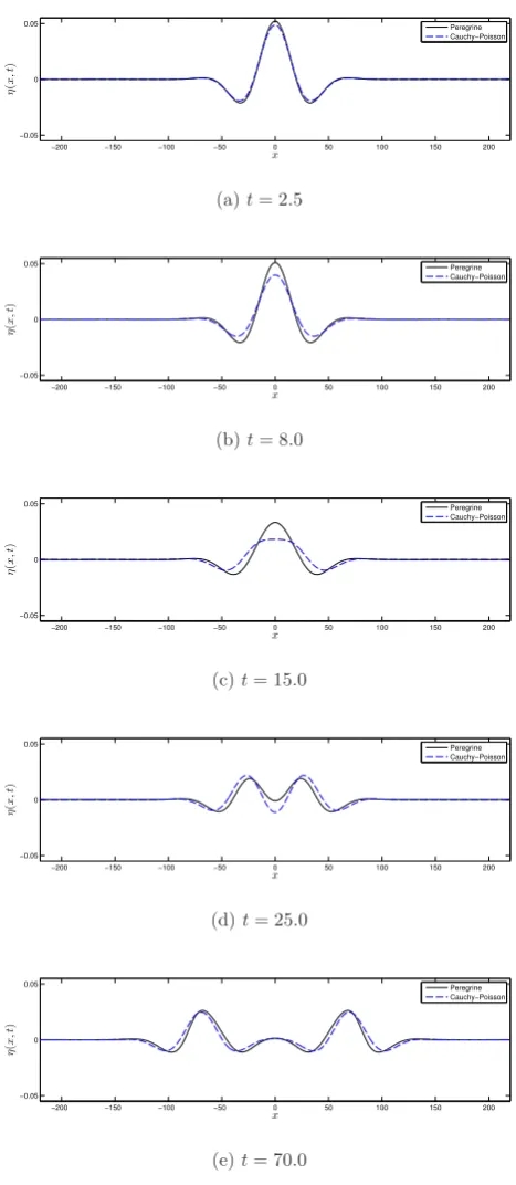
Figure 10. Free surface waves generated by a fast bottom motion. The blue
dashed line corresponds to the analytical Cauchy–Poisson solution, while the solid black line is our numerical solution to the Peregrine system.
Fig. 10. Free surface waves generated by a fast bottom motion. The
blue dashed line corresponds to the analytical Cauchy–Poisson so-lution, while the solid black line is our numerical solution to the Peregrine system. The time snapshots are taken att=2.5,t=8,
D. Dutykh and H. Kalisch: Boussinesq modeling of underwater landslides 279
D. Dutykh & H. Kalisch 24 /33
x
z
0 50 100 150 200 250
−20 −15 −10 −5 0 5
(a)
x
z
5 10 15 20
−20 −15 −10 −5 0 5
(b)
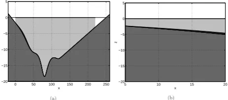
Figure 11.The physical setup of the problem. The river bed is indicated in dark grey. The computational fluid domain is shaded light grey, and the landslide is visible in black. Note the difference in horizontal and vertical scales in the left panel. The right panel shows a closeup of the left beach and part of the landslide in a one-to-one aspect ratio.
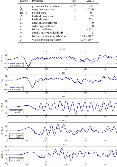
x= 40 andx= 60 show similar waveheights for both the shallow-water, and the dispersive system, but a qualitative divergence, as small oscillations are already developing which are not captured by the shallow-water system. Once the waves have propagated to the wave gauges located atx= 80, the dispersive oscillations have amplified, so that the waveheight is larger by a factor of 2 to 3 than the waveheight predicted by the shallow-water system. Going further to the wave gauges located atx= 100 andx= 120, the now rising bottom starts to have a damping effect on the waves.
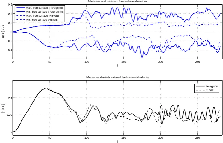
The maximum and minimum free surface elevation over the whole domain is shown in Figure
13. On the lower panel of the same Figure13we show the maximal unsigned horizontal velocity. One can see that for short times the hydrostatic and dispersive models give very close extreme values. Later the differences start to appear due to the accumulation of dispersive effects.
Figure14shows the development of the kinetic energy of the landslide mass and simulta-neously the total (kinetic plus potential) energy contained in the body of the fluid and the surface waves. Energy development is an important question in the study of tsunamis, and there have been studies exclusively devoted to this question [60]. Energy issues connected to water wave models of Boussinesq type have also been studied before [1,2,20]. While these models contained a source of energy, in the case at hand, the work done by friction as the landslide slides down the bottom acts as a drain of energy, and after the landslide has come to rest, all energy has been transferred to the fluid. However, not all energy can be considered as residing in the wave motion, because a significant amount of energy is needed to lift the water from the final position of the landslide to the initial position of
Fig. 11. The physical setup of the problem. The riverbed is
indi-cated in dark grey. The computational fluid domain is shaded light grey, and the landslide is visible in black. Note the difference in hor-izontal and vertical scales in the left panel. The upper panel shows a close-up of the left beach and part of the landslide in a one-to-one aspect ratio.
6 Numerical results
Let us consider a one-dimensional computational domain
I= [a, b] = [0,220] composed of two regions: the genera-tion region and a sloping beach on the right. More specif-ically, the static bathymetry function h0(x) is given by a
smoothed out profile generated from the expression
h0(x)=
d0+tanδ(x−a)+p(x), a≤x≤m,
d0+tanδ(m−a)−tanδ(x−m), x > m,
where the functionp(x)is defined as
p(x)=A1sech(k1(x−x1))+A2sech(k2(x−x2)).
In essence, this function represents a perturbation of the sloping bottom by two underwater bumps. We made this nontrivial choice in order to illustrate the advantages of our landslide model, which was designed to handle general non-flat bathymetries. The parameters can be chosen in order to fit a given bathymetry, but the particular values used here are A1=4.75, A2=8.85, k1=0.06, k2=0.13, x1=45,
x2=80, andm=120. The bottom profile for these
parame-ters is depicted in Fig. 11. Of course, in general, if the bot-tom topography is known, the