https://doi.org/10.5194/dwes-10-53-2017 © Author(s) 2017. This work is distributed under the Creative Commons Attribution 3.0 License.
Technical note: Efficient online source identification
algorithm for integration within a contamination
event management system
Jochen Deuerlein, Lea Meyer-Harries, and Nicolai Guth
3S Consult GmbH, 76137 Karlsruhe, Germany
Correspondence to:Jochen Deuerlein ([email protected]) Received: 17 March 2017 – Discussion started: 21 March 2017
Accepted: 6 June 2017 – Published: 17 July 2017
Abstract. Drinking water distribution networks are part of critical infrastructures and are exposed to a number of different risks. One of them is the risk of unintended or deliberate contamination of the drinking water within the pipe network. Over the past decade research has focused on the development of new sensors that are able to detect malicious substances in the network and early warning systems for contamination. In addition to the optimal placement of sensors, the automatic identification of the source of a contamination is an important com-ponent of an early warning and event management system for security enhancement of water supply networks. Many publications deal with the algorithmic development; however, only little information exists about the inte-gration within a comprehensive real-time event detection and management system. In the following the analytical solution and the software implementation of a real-time source identification module and its integration within a web-based event management system are described. The development was part of the SAFEWATER project, which was funded under FP 7 of the European Commission.
1 Introduction
Drinking water distribution networks (WDNs) are an inte-gral part of the technical infrastructure. Their task is to de-liver a sufficient amount of drinking water of perfect qual-ity at any place and any time. Since WDNs are exposed to a number of different risks, they belong to the critical infras-tructures. One important risk is the (deliberate) contamina-tion of drinking water with harmful substances. An adequate risk management system is required to manage the different threats in case of an event. Such a system normally consists of components for prevention, detection and response. Pre-vention measures include for example the protection of facil-ities such as water treatment plants, storage tanks and pump-ing stations or network sectorization for isolation of contam-inants (Di Nardo et al., 2014). Among others, online mon-itoring of water quality within the distribution system is an essential part of a contamination warning or early detection system (Hall et al., 2007). As important, in case of a con-tamination event, is a well-prepared and efficient response
For solution of the source identification problem there are several categories of formulations and solving methods. Tra-ditionally, SI was treated as an inverse parameter estimation problem. The parameters are the node time pairs of possible contaminations. Laird et al. (2005) formulated the SI lem as a non-linear, infinite-dimensional optimization prob-lem subject to algebraic, ordinary differential, and partial dif-ferential constraints. Input parameters are the flow profiles calculated by hydraulic simulation and measured concentra-tions at sensor locaconcentra-tions. As output, the time-dependent con-centration along pipes and at junctions and the mass input at junctions as a function of time are sought. The method was tested for a network with 469 nodes. Even for this small model the number of unknowns in the non-linear program-ming (NLP) problem already reached 210 000. As a con-sequence, the method cannot be applied to real-time calcu-lation of the large-size network models. Other authors use stochastic optimization methods for solution of the param-eter estimation problem. Preis and Ostfeld (2008) combine the EPANET hydraulic and water quality simulation soft-ware with a genetic algorithm (GA). The objective function consists of a least squares function of measured and calcu-lated concentrations. For the measurements, imperfect sen-sors are also taken into account. The calculation time for a test network with less than 1000 nodes was about 1 h. Liu et al. (2011) use an evolutionary algorithm (EA) for adap-tive dynamic optimization (based on updated observations) and continually search for optimal solutions of a modified least squares function. Other authors (e.g. Propato et al., 2007) propose applying an input–output model for contam-inant source identification. The model consists of a linear relationship between the possible source concentrations and the concentration measured at the sensors. The equation uses a linear transport matrix that is, in general, underdetermined, leading to non-unique solutions. Since for real-time applica-tion the execuapplica-tion time of the method is the critical perfor-mance indicator, optimization-based methods are not suited. Therefore, De Sanctis et al. (2010) use a modified particle backtracking method (PBA) for identification of all possible contaminant source locations. For alarm generation, binary sensor information is introduced. The authors claim that for-mulating the SI problem as an inverse water quality problem is difficult for three reasons: (1) ill-posedness (sparse sensor grid in contrast to a huge number of possible sources, e.g. hydrants, house connections), (2) problem size (number of possible sources times the number of time steps within the detection time), and (3) assumption of the existence of per-fect quality sensors that are capable of measuring the concen-tration of all relevant substances that do not exist in reality. In addition to the available number of sensors and their reliabil-ity, the design of the sensor network is also essential for the effectiveness and accuracy of the source. Recently, a method was published that takes into account the feedback between the sensor network design and the efficiency of the source identification algorithm (Ung et al., 2017).
In the following a software tool is presented that is suitable for real-time application and integration within risk or event management systems. It was developed as part of EU-funded project SAFEWATER (contract number: 312764). The algo-rithmic development is based on a simplified transport al-gorithm that runs forward and backward in time. Whereas backtracking is used for source identification, forward sim-ulation delivers the estimated current spread of contamina-tion based on the source locacontamina-tions. As a possible response action, the tool also proposes valves to be closed for isola-tion of contaminants. The software is part of comprehensive event management software (EMS) that collects all informa-tion from the field and from different software components that are connected with the EMS, including a newly devel-oped event detection system (EDS) as well as offline and on-line hydraulic and water quality simulators. The paper starts with an overview of the theoretical background, including a simplified transport model and source identification algo-rithm. Then, the integration within the EMS framework is outlined. Finally, the application of the tool is presented for the SAFEWATER test lab water network at Water Supply Zurich.
2 Theoretical background
2.1 Transport model
The theory of modelling reaction and transport of substances within a water distribution system is described in a number of books and articles. A good overview of the methods that are included in most of the commercially available simulation software tools can be found in Rossman and Boulos (1996). In the following a very brief presentation of the problem of contaminant injection with sharp quality fronts (discontinu-ity) is given. Reaction and diffusion are not considered here. In this case the transport is described by the so-called Rie-mann problem (p. 49 in Toro, 2009):
(PDE) ct+vcx=0, −∞< x <∞, t >0, (1a)
(IC) c(x,0)=c0(x)=
cL if x <0,
cR if x >0. (1b)
case of Riemann problems (Eq. 1) is
c(x, t)=c0(x−vt)=
cL if x−vt <0,
cR if x−vt >0. (2)
For the Riemann equation, the characteristic that passes through x=0 is of special interest. It separates the (con-centration) surface above thex–t-plane into one part where the concentration is cL and one part where the concentra-tion iscR. This particular characteristic line is the only one across which the concentration changes. For implementation, the IVP (1) is solved for all pipes using a MOC. For later processing of the results, the traces of a particle that travels along the special characteristic line that starts fromx=0 is stored. In the easiest case the flow velocity is constant and only the slope has to be stored. However, in extended pe-riod simulations the flow velocity and even the flow direction may change from external time step to time step. Therefore, it proved to be convenient to store the [time, position, value] triples of all particles for every external time step. The term external time step refers to the time interval between updates of the boundary conditions of the underlying hydraulic simu-lation model. Since the flow velocities change only after such an external time step, the full information [value, time, posi-tion] can be re-established from this information for any time and location.
In order to move from the pipe level – with the initial as-sumption of infinite pipe length from above – to the network level, additional boundary conditions have to be considered for a finite pipe length. The IVP then is transferred to an IBVP (initial boundary value problem). In general, the com-bination of pipes at a junction requires the formulation of ad-ditional mixing conditions at network nodes. Since no criti-cal concentration can be given for unknown substances, here, the binary information (contaminated yes/no) of the front is transferred unchanged to all pipes having outflows from the junction.
2.2 Source identification
The proposed source identification (SI) module is distin-guished from existing solutions by its real-time capabilities, its integration within the EMS and the permanent calculation of the monitoring state of the sensor network even in the case with no alarm. The latter is useful especially when flow di-rections change due to network operations. The continuous backtracking of negative sensor alarms allows the visualiza-tion of the current monitoring state of the system. For any location in the network, the last time of observation is calcu-lated. Given the limited coverage of the distribution network by the sensor network, a contamination may not be detected by the sensors because it can be outside of the covered area. It is important to be aware of this issue if other detections, like customer complaints, indicate an event contradicting the negative alarm states of the sensors.
In the context of SAFEWATER, one basic requirement was that the source identification algorithm must deliver results almost in real time. For that reason, all kinds of optimization-based approaches (see the Introduction) are not suitable due to the huge number of simulations and thus the long computing time that are required for stochastic opti-mization models. Therefore, a more direct approach was cho-sen for the solution of the inverse problem. It has some sim-ilarities to the particle backtracking algorithm that was first presented by Shang et al. (2002) and the approach presented by De Sanctis et al. (2010). Its core component is an event-driven simplified transport algorithm that does not consider reaction and diffusion mechanisms as described in the previ-ous section. Another key performance indicator is the usage of memory. In the presented approach, a special format was developed that is used for storing the characteristic lines of the transport equation MOC. This information can then be used for particle tracking (forward and backward) as well as reconstruction of time curves (at a certain location) or the concentration along a pipe at a certain time. For implemen-tation in SAFEWATER, an event-driven method is used that strongly simplifies the common water quality equations: in-stead of concentrations, only binary quality states are calcu-lated (contaminated/not contaminated), neglecting reaction and diffusion terms and using simplified mixing equations. An event is triggered every time a change in the (binary) boundary conditions occurs (for example, start of intrusion in the forward case or release of a sensor alarm in the backward case). The algorithm sends a separator front through the sys-tem following the flow velocity of the water in the pipes (for-ward) or working against it (backtracking case). The mov-ing front separates the network into regions that have distinct values for the binary quality state (contaminated/not contam-inated). In the reverse case, a change in the sensor alarm state is considered a binary signal (no alarm → alarm). Based on this simplifying assumption, memory requirements and calculation time are minimized in comparison with common water quality solvers. The fact that in the case of a real event the substance and input concentration of a contamination are presumably not known may serve as a justification for the simplifying assumptions.
lo-cations. Based on a worst case assumption a unique source location is selected that serves as input for a simplified look-ahead transport calculation that gives an estimation over the future spread of contamination. As a worst case, the node with the biggest outflow volume is chosen. This second step is necessary since the backtracking algorithm in general does not give unique results. The region of possible source loca-tions can be quite large depending on the efficiency of the sensor network.
It is important to mention that negative sensor alarms also deliver useful information. The backtracking of nega-tive alarm states (under the assumption of perfect sensors) identifies the nodes upstream of these sensors and the times when the signal passes the nodes. A contamination starting from such a node before the calculated arrival time of the negative separator front is not possible since, in this case, the sensor alarm state must have been positive as well. Conse-quently, the nodes can be withdrawn from the list of source candidates. Another important application of backtracking of negative sensor alarms consists in the continuously updated monitoring state of the system. The backtracking algorithm calculates a kind of reverse water age for each location under the protection of the sensor network. That means that for any location the time of the last observation is known. In addi-tion, the nodes and pipes that are not covered by the sensor network can be visualized and updated in real time.
For estimation of the future spread of contamination and the identification of isolation valves, the simplified forward transport calculation is used. Here, the assumption is again that more complicated water quality calculations such as in-complete mixing, reaction and diffusion are of secondary im-portance for this particular problem. It is expected that at the beginning of a real contamination event the kind and severity of the substance are unknown. In the SAFEWATER project a second water quality solver was implemented that deals with all of these issues. Once more information about the chemical properties of the agent is available, the enhanced water quality solver can be used for more detailed calcula-tion of concentracalcula-tions.
3 Outline of the integration within the EMS
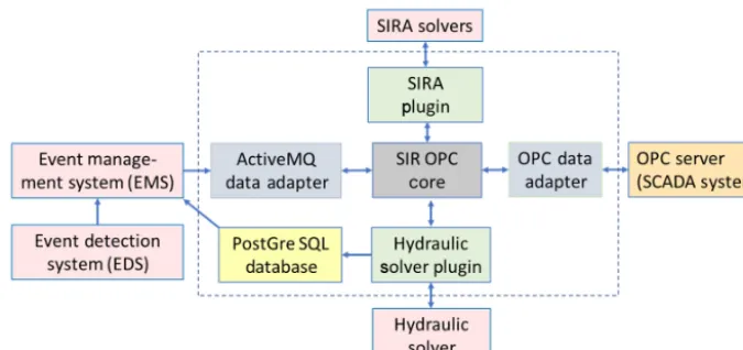
For integration of the different software components within a real-time environment and the SAFEWATER-EMS, the ex-isting SirOPC software tool was extended by implementation of additional plugins. Originally, SirOPC was developed for connecting hydraulic simulation software with common OPC server software provided by the SCADA system for receiving and sending real-time operational data. The plugin technol-ogy allows the flexible extension of the software. For connec-tion with external data, adapter plugins are used (blue boxes in Fig. 1). Application plugins allow the integration of spe-cialized software tools (green boxes in Fig. 1) with the data managed by the core component. The plugins provide the
in-terfaces between the central data and native applications. For example, the hydraulic solver plugin includes the interface for updating boundary conditions of a hydraulic simulation model with SCADA system data that are delivered through SirOPC and the OPC data adapter. The SIRA plugin is used to connect the source identification solver with the core soft-ware and manages the update of the flows calculated by the hydraulic solver. For exchange of mass data, an additional database interface exists. For communication with the EMS, an ActiveMQ (2015) data adapter plugin has been developed in the project that is able to receive messages about changes in alarm states of the sensors that are detected by the EDS. Based on this information, the online variables are updated in the SirOPC core, from where the information is transferred to the SI algorithm. By implementation, the developed SI mod-ule runs in combined online mode together with the hydraulic solver. The boundary conditions of the hydraulic solver are updated in regular time intervals by receiving data from the OPC server. After each time step calculated by the hydraulic solver, the flow velocities in the source identification algo-rithm are updated and new backtracking calculations are car-ried out. Positive alarms are generated by the EMS as soon as a pending alarm is acknowledged by the operator. Alarms could trigger calculations automatically, but in order to avoid false alarms due to known events, at this stage of the devel-opment every alarm has to be manually acknowledged. After that, an ActiveMQ message is sent to SirOPC. The next SI calculation considers the positive alarm and calculates the possible locations for the source of contamination that are consistent with the alarm states of all sensors, including neg-ative sensor alarms.
As a possible response action, the valves are identified that have to be closed for isolation of the contaminant. The results of the different algorithms are presented in a native GUI of the SI application as well as in the EMS map. The execution loop, which is in mutual feedback with the hydraulic simu-lator, is controlled by so-called custom commands, a kind of virtual state machine (Petri-Net). The results of the SI calcu-lations are stored in a database that can be accessed by the EMS for further processing and visualization.
4 Source identification module example
4.1 Calculation of source candidates
Figure 1.System architecture of SI integration within the SAFEWATER event management system.
Figure 2.Test network with four sensors (orange circles) and contamination source (red circle).
the OPC server through a bidirectional interface provided by the SirOPC online OPC client. The hydraulic simulation runs every 5 s with updated boundary values from the OPC server. The calculation results, namely the flow velocities, are stored in a native binary data format from where they can be accessed by the SI plugin and transferred to the transport solvers.
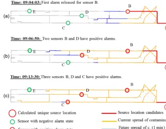
Water quality sensors are installed at five locations. Four sensors are distributed over the network (orange circles) and one is located directly downstream from the contamination source (red circle) in order to control the entrance water qual-ity for the injection scenarios. For demonstration purposes, the sensor alarm times were calculated by running a forward transport calculation that starts at 09:02. The SI software tool is able to record the earliest time when the contamination passed the sensors. During the tests, a valve on the lower left-hand side was closed. Therefore, there is almost no flow in direction towards sensor E and the alarm time is beyond the scenario end time (09:30). The subsequent alarm times are also shown in Fig. 2. From Fig. 3 it can be seen that the more information is available (through subsequent additional alarms), the smaller the area of possible source candidates (red marked pipes). In Fig. 3a all pipes upstream of sensor B
are possible locations. In Fig. 3b the combination of the up-stream pipes of sensor B and of sensor D decreases the set of source candidates because the locations directly upstream of sensor B cannot explain the alarm at sensor location D. The area is further reduced after the third alarm (Fig. 3c). Possi-ble source locations must also be upstream of sensor C. The orange and blue marked pipes show the estimated spread at the current time and in a predefined look-ahead time, respec-tively.
4.2 Impact of negative sensor alarms on source
Figure 3.Sequential release of sensor alarms and results of the SI algorithm, current spread of contaminant and look-ahead.
and no signal of negative sensors can be found for these loca-tions. A particular weighting scheme has been implemented, considering also the duration and time delay between the dif-ferent signals. The criterion for a node to be a source can-didate location is that all signals that passed that node are positive signals. The set of source candidate locations con-sists of a more or less large area, depending on the design of the sensor network, the number of sensors and the topology of the network graph. For example, if forward calculations shall be carried out for the estimation of the current spread of contamination, a single source node has to be selected.
5 Conclusions
In case of a contamination event, finding fast, efficient and simple response actions after detection is the key issue for mitigating contamination of drinking water distribution net-works. The online source identification module indicates the possible locations of the source of contaminants and shows the current monitoring state at any location and any time. The presented SI module is integrated in combination with hydraulic online simulation within the SAFEWATER event management system. On the SI input side the hydraulic on-line simulator delivers system-wide flow velocities needed for transport calculations based on actual process data that are received from a SCADA system using OPC technology. The continuous update of the model by online data aims at maintaining a sufficient match between the model
parame-ters and the real situation in the field for changing opera-tional conditions. This is a step forward and improves the situation compared to calculations based on offline models. However, it must not be forgotten that uncertainty in model parameters still exists, especially the demands, affecting also the accuracy of the results of the source identification algo-rithm. The number of unknown parameters normally exceeds the number of measurements by magnitude. The alarm states of sensors are sent by the EMS using the ActiveMQ com-munication channel. As output, the module generates current monitoring states of the network and, in the case of a posi-tive sensor alarm, the source candidate locations. The output is visualized in the GIS map of the EMS. In addition to the tests for the network on a lab scale, the functionality and ap-plicability of the development of the approaches were also proven within the project for three pilot zone systems of real existing networks (details cannot be presented for security reasons). Future work should focus on the enhancement of the calculation cycle. While the run time of the algorithms is considered to be sufficiently short also for large networks, the huge amount of data to be processed and transferred through the different modules is still a challenge for large real-world applications.
Advisory Group) project. The motivation for and the objectives and achievements of the SAFEWATER project can be viewed at https://www.youtube.com/watch?v=Bs5SljKUxgE.
Competing interests. The authors declare that they have no con-flict of interest.
Special issue statement. This article is part of special issue “Computing and Control for the Water Industry, CCWI 2016”. It is a result of the 14th International CCWI Conference, Amsterdam, the Netherlands, 7–9 November 2016.
Acknowledgements. The SAFEWATER project has re-ceived funding from the European Union’s Seventh Framework Programme for research, technological development and demon-stration under grant agreement no. 312764.
Edited by: Edo Abraham
Reviewed by: two anonymous referees
References
ActiveMQ: available at: http://activemq.apache.org, last access: 23 May 2017.
Chang, N. B., Pongsanone, N. P., and Ernest, A.: Comparisons be-tween a rule-based expert system and optimization models for sensor deployment in a small drinking water network, Expert Syst. Appl., 38, 10685–10695, 2011.
De Sanctis, A., Shang, F., and Uber, J.: Real-time identification of possible contamination sources using network backtracking methods, J. Water Res. Pl.-ASCE, 136, 444–453, 2010. Di Nardo, A., Di Natale, M., Msumarra, D., Santonastaso, G. F.,
Tzatchkov, V., and Alcocer-Yamanaka, V. H.: Dual-use value of network partitioning for water system management and protec-tion from malicious contaminaprotec-tion, J. Hydroinform., 17, 361– 376, https://doi.org/10.2166/hydro.2014.014, 2014.
Hall, J., Zaffiro, A. D., Marx, R. B., Kefauver, P. C., Krishnan, E. R., Haught, R. C., and Herrmann, J. G.:. On-line water quality pa-rameters as indicators of distribution system contamination, J. Am. Water Works. Ass., 99, 66–77, 2007.
Laird, C. D., Biegler, L. T., Bartlett, R. A., and van Bloemen Waan-ders, B. G.: Contamination source determination for water net-works, J. Water Res. Pl.-ASCE, 131, 125–134, 2005.
Liu, L., Ranjithan, S. R., and Mahinthakumar, G.: Contaminant source identification in water distribution systems using an adap-tive dynamic optimization procedure, J. Water Res. Pl.-ASCE, 137, 183–192, 2011.
OPC Foundation: OPC, available at: https://opcfoundation.org, last access: 23 May 2017.
Preis, A. and Ostfeld, A.: Genetic algorithm for source characteriza-tion using imperfect sensors, Civ. Eng. Environ. Syst., 25, 29–39, 2008.
Propato, M., Tryby, M. E., and Piller, O.: Linear algebra analysis for contaminant source identification in water distribution systems, World Environmental Water, Tampa, Florida, USA, ASCE, 1–10, 2007.
Rossman, L. and Boulos, B.: Numerical methods for modeling wa-ter quality in distribution systems: a comparison, J. Wawa-ter Res. Pl.-ASCE, 122, 137–146, 1996.
Sandia National Laboratories: CANARY, available at: https:// software.sandia.gov/trac/canary, last access: 23 May 2017a. Sandia National Laboratories: TEVA-SPOT, available at: https://
software.sandia.gov/trac/spot/, last access: 23 May 2017b. Shang, F., Uber, J. G., and Polycarpou, M. M.: Practical
back-tracking algorithm for water distribution systems, J. Environ. Eng., 128, 441–450, 2002.
Toro, E. F.: Riemann Solvers and Numerical Methods for FLuid Dynamics – A Practical Introduction, 3rd Edn., Springer, Berlin Heidelberg, Germany, 2009.