- 40 -
Abstract—Sensing is a fundamental function in wireless sensor networks. Researchers have built WSN platforms with a wide spectrum of sensors, ranging from simple thermostats to micro power impulse radars. Traditional signal processing algorithms, however, often prove too complex for energy-and-cost-effective WSN nodes. In this work, we propose a distributed approach for event classification in wireless sensor networks. This approach is based on the assumption that events to be detected can be characterized by a set of features where each can be measured by a specific kind of sensors. The paradigm is composed of two phases: a training phase and a classification phase. In the training phase, for each event type E and a feature F, a set of values is determined. Then, in each node with a sensor corresponding to a feature F we maintain a 2-dimensional array where columns represent event types and rows represent the divisions in the readings’ range of the corresponding sensor. In the classification phase, the network detects and classifies events in a distributed fashion using a voting-like technique in which individual nodes contribute to the classification. Our algorithms are validated through extensive simulations and analysis.
Index Terms—Sensor Networks, Pattern Recognition, Event Classification, Energy Efficient.
I. INTRODUCTION
A wireless sensor network is a network composed of numerous independent sensor nodes which are small devices consisting of a radio transceiver, sensors, microcontroller and an energy source which is a battery. These nodes have limited energy sources, memory, computational capabilities and bandwidth. Due to the mobility of nodes, their limited powers and possible failures, the network topology is dynamic. Hence, such networks do not have a fixed and centralized infrastructure. Randomly distributed nodes over a sensor field in a WSN communicate with each other and with external media or devices known as command nodes through sensor gateways.
Sensor nodes have power and bandwidth constraints and consequently communication between nodes requires the use of intermediate nodes; this adds a new functionality to sensor nodes that is data routing. A number of routing protocols have been developed to accommodate with the dynamic changes of WSNs where:
1) The network topology is dynamic and sensor nodes self-organize themselves.
2) A node may leave or join the network arbitrarily.
Manuscript received November 9, 2008.
Rawad Abu Assi is a graduate student at the American University of Beirut, Beirut, Lebanon.
Mohamed K. Watfa is a professor at the Computer Engineering department in the University of Wollongong, Dubai, UAE.
3) Links may be broken. 4) Nodes may die.
5) Nodes’ power and energy may decrease and thus they cannot be relied upon.
Wireless Sensor Networks (WSNs) provide flexible sensing capability with a large number of low-power and inexpensive sensor nodes. The selection and integration of sensors on a WSN platform is often a manageable task given a certain amount of engineering effort. The situation is, however, completely different above the physical sensor and computing hardware layer. The acquisition and processing of sensor data impose great challenges on WSN design because of strict resource constraints. Cost-effectiveness being an important objective, WSN designers often choose mass produced commercial off the shelf (COTS) sensors when designing a sensor network system. Moreover, a sensor node must be energy efficient. As a result, the raw sensor data is often of low-quality – they are not always reliable, not always repeatable, usually not self-calibrated, and often not shielded to environment and circuit board noise. Obviously, it is necessary to use signal processing algorithms to filter, process, and abstract sensor data with software to provide precise, reliable, and easy-to-use information to applications. Traditional signal processing algorithms, however, often prove too complex to implement on inexpensive sensor network hardware without digital signal processing co-processors.
Event detection and classification in wireless sensor networks is a relatively new research topic. What makes it more challenging is the conflict between the complex computation required by the state-of-art classification algorithms and the scarce resources available in wireless sensor networks. In this paper, we propose DEFACTO, a distributed algorithm with two phases for event classification in wireless sensor networks, which tries to overcome this problem. The rest of the paper is organized as follows. Section 4 presents an overview of related work on event detection and classification in wireless sensor networks. Section 3 presents the DEFACTO algorithm with an elaboration on the two phases. In Section 4, we evaluate our paradigm by defining the metrics we used and the simulation results we got. Finally, we conclude with some perspectives and future work.
II. RELATED WORK
With the development of WSN systems, sensing, detection, and tracking have been a prosperous research area. Specifically, in [1], the authors used Gaussian classifiers to track and classify targets based on their temporal and spatial signature. [2] proposes a hierarchical architecture which
DEFACTO: Distributed Event ClassiFicATiOn
in Wireless Sensor Networks
distributes classification functions among individual nodes, groups of nodes and the base station. Each classification level is supported with a classifying algorithm based on the collected data. In [3], the authors propose a recognition system specialized with vehicle classification. It uses rough neural networks to overcome the problem imposed by the time-variation and uncertainties of acoustic measurements. [4] uses feed forward neural networks with one hidden layer to estimate a certain measurement in one region using measurements obtained elsewhere in order to achieve energy savings. In [5], the main goal is dimensionality reduction, so the authors used Adaptive Resonance Theory (ART), a neural network model, to do so. Each sensor node contains several sensors and uses the ART applied in it to send a single output.
Wang et. al. studied acoustic tracking using Mica motes [10]. Simon et. al. designed a sniper localization system with acoustic signal processing [11] and accomplished good performance. These systems employ special powerful nodes or DSP co-processors to process acoustic data. Zhao et. al. described collaborative signal processing [12] to retrieve more accurate information from sensor data and achieve better target tracking performance. Pattem et. al. build a framework to evaluate the tracking strategies in an energy aware context [13]. Most of the performance analysis in [12] and [13] are conducted by simulations, concentrating on exploring the design space and trade-offs under specific constraints and assumptions. Along the direction of real-world application and deployments, researchers have also constructed a number of successful systems. Szewczyk et. al. [14] developed a habitat monitoring WSN on the Great Duck Island and the system operated for months. Zhang et. al. developed a WSN for wild life tracking [15]. These systems demonstrate the flexibility and capability of the WSN technology in various applications. However, sensor networks might face more demanding application requirements. As a result, many design choices are different in these systems. For example, many current systems typically employ centralized processing which is not feasible in many surveillance networks.
In [16], the authors describe a surveillance network that can detect moving targets. The system uses Mica2 motes equipped with a magnetometer (Honeywell HMC1002), an acoustic sensor and, on some nodes, a motion sensor. The motion sensor is an Advantaca MIR (micropower impulse radar) sensor which transmits microwave signals and detects motion by capturing distortion of the reflected signal. The network reports a target as a walking person or a vehicle. Therefore, it has a preliminary classification capability. However, there is very limited signal processing in it. As a result, the classification is limited in both functionality and performance. Also, the MIR sensors, worth four thousand dollars each, are not a typical choice for energy-and-cost-effective systems.
Brooks et. al. [1] introduced a collaborative signal processing framework for sensor networks using location-aware routing and collaborative signal processing. Their study provides many insights into the distributed collaborative classification in WSNs. Nevertheless, the CSP framework involves non-trivial training and computation
overhead, which our system cannot afford. Also, the system implementation and evaluation of the CSP framework
employ nodes with higher power than the
energy-and-cost-effective WSN nodes a network system is targeting. In fact, their work must satisfy three conflicting requirements simultaneously – low-end hardware, long lifetime, and sophisticated function. This challenging design context is different than what past solutions assume.
Some interestingly deployed sensor networks include the Extreme Scaling project which is similar to VigilNet in functionality and hardware platform [8, 9]. However, a major difference is that the Extreme Scaling WSN employs a heterogeneous network topology and uses a more powerful Stargate node for some computation and communication intensive tasks.
III. DEFACTO
Given a wireless sensor network with N randomly deployed and static nodes with different kinds of sensors and a set of M events to be detected, the aim is to find a methodology that allows the WSN to detect and classify any of the M events once it occurs. First, we distinguish between three entities: event-type: for example a human, a vehicle, etc.
Event: This is an instance of event-type. For example: Bob, Bob’s car, etc. Feature: A characteristic that can be measured with a sensor. For example: intensity, humidity, etc. Mark: A sensor reading for a certain feature F when applied on an event. For example, the intensity of an event e is 3.5. DEFACTO is divided into two stages: a training stage and a classification phase. In what follows we elaborate on both phases.
A. Training Phase
In this stage, for each event-type E and for each feature F, we extract marks of E by getting sensor readings of the feature F from events of type E. All the events whose marks are extracted will be called training events. We associate with each sensor type i a range of readings Li and we partition this
range into divisions of width δi. The value of δi depends on the precision required to identify events of different types by the sensor. For example, if two events of different types can have close values then δi should be small. For each sensor type, we maintain a 2-dimensional table whose columns correspond to the event types and whose rows correspond to the divisions of the corresponding sensor’s reading range. We will call this table the classification table. The value in cell (i, j) represents the percentage of training events belonging to event-type j among those whose marks lie in division i. The table in figure 1 is an example. Assume that the sensor is an intensity sensor and its reading range is 50. Also assume that the divisions have a width of 10 and that we have 3 event types E1, E2, and E3. For example, the first row
indicates that 70% of the training events whose intensity value lies between 0 and 10 are of type E1.
B. Classification Phase
- 42 - waits for a random time Ti. If Ti expires before receiving any
message, it enters the initiating state and sends a broadcast classification message having the format in figure 2 to all the neighboring nodes. In this case, the node becomes the source of the event and it will be simply called the source.
E1 E2 E3
0-10 0.7 0.1 0.2
10-20 0.3 0.3 0.4
20-30 0.1 0.0 0.9
30-40 0.0 1.0 0.0
40-50 0.5 0.4 0.1
Fig. 1 An example classification Table
The purpose behind Ti is to avoid the case when several
nodes send their message at the same time if they detect the same event at the same time. The first field in the message represents the id of the source. The message-id is generated by the source to distinguish the current event from those that might be detected in the future. In addition, the source adds its location to the message. The first three fields will be the same in all subsequent messages. nb_votes represents the number of nodes which will contribute to the classification (initially N is 0). Each node that will contribute to the classification will select from its classification table the row corresponding to its sensor reading. The row field represents the summation of all such rows (initially the row field contains the row selected by the source).
source-id message-id Source
location nb_votes row Fig. 2 Broadcast classification message.
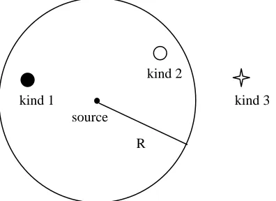
We will consider two parameters R and S which are application-dependent. R represents the radius of the minimal region in which the event can be detected and S represents the minimal acceptable number of nodes contributing to the classification so that the decision is reliable. There are three kinds of nodes that receive the message sent by the source (figure 3): Nodes of kind 1 are those which detected the same event and they are within a range of R with the source. Nodes of kind 2 are those within a range of R but didn’t detect any event, and nodes of kind 3 are outside the range of R.
After receiving the message from the source, a node of kind 1 waits for the random time Tv and if Tv expires before
receiving any message the node enters the voting phase. It increments N and adds the row it selects from its classification table to the row field and then it forwards the message by broadcasting it. If before Tv expires the node
received a message, it waits for another Tv and the process
repeats in a similar fashion.
Fig. 3 Kinds of nodes receiving a broadcast classification message.
It’s important to note that determining the kind of subsequent nodes is done with respect to the source node and not with the node that forwards the message. Another important remark is that each node broadcasts a message at most once. When a node of kind 1 receives a message in which the value of N is below S, it increments N and adds the row it selects to the row field and forwards the message. When any node receives a message in which the value of N is higher than S, it searches for the maximum value in row and classifies according to the event-type it represents. If a node of kind 1 receives a message it has already forwarded, it discards it. Nodes of kind 2 and kind 3 discard the message. The state transitions in DEFACTO are shown in figure 4.
IV. EVALUATING DEFACTO
A. Evaluation Metrics
To evaluate DEFACTO, we considered three metrics:
accuracy, communication overhead, and percentage of wrong classifications. Accuracy is the percentage of events classified successfully among all the events injected in the network. We defined communication overhead as the average number of messages broadcast per injected event. Finally, percentage of wrong classifications is defined as the percentage of events classified wrongly with respect to the total number of classified events. Note that some of the injected events were not classified.
B. Event Definition
Because of the lack of real data, the only solution was to generate random data. But doing this with no constraints on the generated data will be meaningless and thus we won’t be able to analyze the performance of DEFACTO. For this sake, we used two constraints: a mean value and a deviation.
For each event type Ei and each feature Fj, we define a mean value mij and a deviation value devij. All the training events of type i has their values of feature j as random numbers in the interval [mij-devij, mij+devij]. If we have n features f1, f2, …, fn, an event of type i which will be injected in the network will be represented by an n-tuple (v1, v2, …, vn) where each vj is a random number in the interval [mij-devij, mij+devij].
source kind 1
kind 2
kind 3
Fig. 4 State transitions in DEFACTO.
C. Simulation Details
For our simulation, we used Jprowler [7] which is Java-based simulator for prototyping, verifying and analyzing communication protocols of TinyOS ad-hoc wireless networks. It supports two radio models: Gaussian (for static nodes) and Rayleigh (for mobile nodes), and one MAC protocol: MICA2 with no acknowledgment. Simulation was done on a 20 by 20 square area. We used two event types and three features.
D. Simulation Results
First, we studied the effect of varying node density on accuracy and communication overhead. All other parameters were fixed. We found that as density increases, accuracy increases (figure 5) but communication overhead increases (figure 6). This is due to the fact that having more nodes means that more nodes will detect the event but more messages will be sent as a result of initiation or forwarding.
0
0.2
0.4
0.6
0.8
1
20
30
40
50
60
70
80
Node Density
A
c
c
u
ra
c
y
Fig. 5 Accuracy vs. Node density.
0 2 4 6 8
20 30 40 50 60 70 80
Node Density
C
o
m
m
u
n
ic
a
ti
o
n
O
v
e
rh
e
a
d
Fig. 6 Communication overhead vs. Node density.
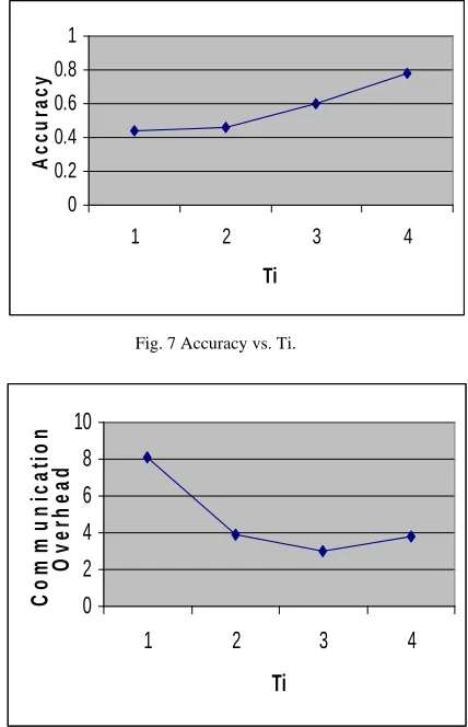
Then we studied the effect of varying the sleep time before initiation Ti on accuracy and communication overhead. We found that as Ti increases, accuracy increases and the
communication overhead decreases. This can be explained by the following: for small values of Ti, the probability of several nodes initiating a message at the same time increases which means that more messages will be initiated and less messages will be forwarded because once a node initiates a message it won’t forward and message received eventually.
0 0.2 0.4 0.6 0.8 1
1 2 3 4
Ti
A
c
c
u
ra
c
y
Fig. 7 Accuracy vs. Ti.
0 2 4 6 8 10
1 2 3 4
Ti
C
o
m
m
u
n
ic
a
ti
o
n
O
v
e
rh
e
a
d
Fig. 8 Communication overhead vs. Ti.
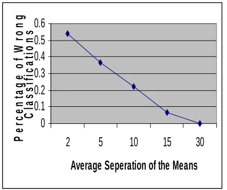
Finally we studied the effect of varying the average distance between the mean values. Since our simulation is based on two event types and three features then we have 6 mean values: m11, m12, m13, m21, m22, and m23. The average mean distance is:
Listening
Wait_For_Initiating
Voting Initiating
Wait_For_Voting Sensor
detects a value
After Ti
A message about the same event is received
After Tv A message
- 44 -
D =( |m11-m21| + |m12-m22| + |m13-m23| ) / 6.
We noticed that as D increases the percentage of wrong classifications decreases (figure 9). This is due to the fact that a higher value of D means a clearer difference between event type.
0
0.1
0.2
0.3
0.4
0.5
0.6
2
5
10
15
30
Average Seperation of the Means
P
e
rc
e
n
ta
g
e
o
f
W
ro
n
g
C
la
s
s
if
ic
a
ti
o
n
s
Fig. 9 Percentage of wrong classifications vs. average separation of the mean values.
V. CONCLUSION AND FUTURE WORK
In this work, we presented DEFACTO, a distributed algorithm for event classification in wireless sensor networks. In the training phase, a classification table is constructed for each feature based on a training set of events with predefined marks. In the classification phase, DEFACTO uses a voting like technique in which nodes detecting the same event collaborate to classify the event based on their classification tables. The simulation results showed that the accuracy of classification increases with node density but with the cost of increased communication overhead.
Also, the results show that the rate of wrong classifications increases as the distance between the mean values of features for different event types decreases. In this work, we restricted ourselves to the case where one event occurs at a time, so our future work will include investigating several events at a time. Also, we will consider the case of n event types rather than 2 types as discussed in simulation. In addition, we will study the effect of using weights such that some features will have more effect on the classification. Another important perspective is to use feedback from wrong classifications to update the classification table so that the process of event classification will be improved.
REFERENCES
[1] R.R. Brooks, A.M. Sayeed. Distributed Target Classification and Tracking in Sensor Networks. In Proceedings of the IEEE, vol. 91 (8), August 2003, pp. 1163-1171.
[2] Lin Gu, Dong Jia, Pascal Vicaire, Ting Yan, Liqian Luo, Aajay Tirumala, Qing Cao, Tian He, John A. Stankovic, Tarek Abdelzaher, and Bruce Krogh. Lightweight Detection and Classification for Wireless Sensor Networks in Realistic Environments. In Third ACM Conference on Embedded Networked Sensor Systems (SenSys 2005), November 2005.
[3] Huang Qi, Xing Tao, and Liu Hai Tao. Vehicle Classification in Wireless Sensor Networks Based on Rough Neural Networks. ACST 2006, pp.141-144.
[4] O. Ozdemir, P. Ray, C. Isik, C. K. Mohan, P. K. Varshney, H. Khalifah, and J. Zhang. Application of Wireless Sensor Networks for AI-Based Monitoring and Control of Built Environments. Innovations and Commercial Applications of Distributed Sensor Networks (ICA DSN) (October 2005).
[5] Andrea Kulakov, Danco Davcev, and Goran Trajkovski. Implementing artificial neural-networks in wireless sensor networks. In Proceedings of IEEE Sarnoff Symposium on Advances in Wired and Wireless Communications, Princeton, NJ, USA, April 18-19, 2005.
[6] Mike Holenderski, Johan Lukkien, Tham Chen Khong. Trade-offs in the Distribution of Neural Networks in a Wireless Sensor Network. Intelligent Sensors, Sensor Networks and Information Processing Conference, 2005. Proceedings of the 2005 International Conference on (2005), pp. 259-264.
[7] http://www.isis.vanderbilt.edu/projects/nest/jpowler
[8] Exscal web site. http://www.cast.cse.ohiostate. edu/exscal/index.php?page=main.
[9] P. Dutta, M. Grimmer, A. Arora, S. Bibyk, and D. Culler. Design of a wireless sensor network platform for detecting rare, random, and ephemeral events. In Proc. of Fourth Intl. Conf. on Information Processing in Sensor Networks (IPSN’05), 2005.
[10] Q. Wang, W. Chen, R. Zheng, K. Lee, and L. Sha. Acoustic target tracking using tiny wireless sensor devices. In Proc. Of 2nd Intl. Conf. on Information Processing in Sensor Networks (IPSN’03), 2003. [11] G. Simon, M. Maroti, A. Ledeczi, G. Balogh, B. Kusy, A. Nadas, G.
Pap, J. Sallai, and K. Frampton. Sensor network-based countersniper system. In Proc. of the 2nd ACM Intl. Conf. on Embedded Networked Sensor Systems (SenSys’04), Nov. 2004.
[12] F. Zhao, J. Liu, L. Guibas, and J. Reich. Collaborative signal and information processing: An information directed approach. Proceedings of the IEEE, 91(8):1199–1209, 2003.
[13] S. Pattem, S. Poduri, and B. Krishnamachari. Energy-quality tradeoffs for target tracking in wireless sensor networks. In Proc. of 2nd Intl. Conf. on Information Processing in Sensor Networks (IPSN’03), 2003. [14] R. Szewczyk, A. Mainwaring, J. Polastre, and D. Culler. An analysis of a large scale habitat monitoring application. In Proc. of the 2nd ACM Intl. Conf. on Embedded Networked Sensor Systems (SenSys’04). [15] P. Zhang, C. Sadler, S. Lyon, and M. Martonosi. Hardware design
experiences in zebranet. In Proc. of the 2nd ACM Intl. Conf. on Embedded Networked Sensor Systems (SenSys’04), Nov. 2004. [16] T. He, S. Krishnamurthy, J. A. Stankovic, T. F. Abdelzaher, L. Luo, R.