Novel Dimensionality Reduction Method for Symbolic Data using Coefficient of Variation

530 | International Journal of Computer Systems, ISSN-(2394-1065), Vol. 02, Issue 12, December, 2015

Available at http://www.ijcsonline.com/

Novel Dimensionality Reduction Method for Symbolic Data using Coefficient of

Variation

Veerabhadrappa

Ȧ

, Lalitha Rangarajan

Ḃ

Ȧ

Department of Computer Science, University College, Mangalore University, Mangalore- 575001, Karnataka, India

Ḃ

Department of Studies in Computer Science,University of Mysore, Manasagangothri, Mysore- 560 006, Karnataka, India

Abstract

In this paper, we propose a novel dimensionality reduction method of representing the set of features using smaller set of

symbolic features. The intersection of intervals of pair samples is computed and using which a similarity value is

generated. For these similarity values, the coefficient of variation is computed which is considered for subsequent

clustering. Experimental results on the standard datasets City Temperature and CORN SOYBEAN show that the

proposed method achieves better classification performance.

Keywords:

Dimensionality Reduction, intersection of intervals, symbolic data, Coefficient of variation,

Association,

disassociation, cluster tendency index.

I.

I

NTRODUCTION

In conventional data analysis, the objects are represented

by numerical vectors. The length of such vectors depends

upon the number of features, which leads to the dataset of

multi-dimensional feature space. As the dimensionality

increases, the problems of analysis and storage increase.

Hence a lot of importance has been attributed to the

process of dimensionality reduction or feature reduction,

which is achieved by sub setting or transformation

methods [12]. Typical data models which are part of the

classification and prediction systems encountered in data

mining may include thousands of variables and databases

with millions of entries. Feature selection based upon a

criterion and feature transformation methods are the two

primary methods of dimensionality reduction. Feature

selection and extraction algorithms seek to provide a lower

dimensional data representation that preserves most of the

available information. Many application domains often

require that knowledge extracted from the data be

comprehensible and compact. Finding the best subset of

variables relevant to the computational model is the goal

of feature selection, while feature transformation

synthesizes new features from the original features.

Symbolic data are extensions of classical data type. In

conventional datasets, the objects are individualized

whereas in symbolic objects they are unified by means of

relationship. Features characterizing a symbolic object

may take more than one value or interval values or may be

qualitative. In real life quite often we come across features

that are interval/duration/spread/span type. In the

conventional data analysis feature vectors of a numeric

type describe samples. However, more generalized

description of samples may be quantitative like intervals,

histograms, sets or qualitative. These complex data types

are termed as symbolic objects. An extension of classical

data analysis methods to such complex data is called

symbolic data analysis. Almost all methods of classical

data analysis are extended to many symbolic objects. The

the error of approximation between the fitted line and the

actual feature values may be more. If the number of

features is too many, a higher order regression curve may

be a better fit, but the reduction of features in this case

may be marginal. In this paper, we propose to transform

the original interval type data into the reduced interval

type data and thereby performing the dimensionality

reduction.

The rest of the paper is organized as follows. Section 2

proposes novel method of transforming the original set of

features to reduced symbolic features. The results of the

experiments conducted to reveal the efficacy of the

proposed method are presented in section 3 and section 4

provides the conclusion

II.

PROPOSED

METHOD

In this section, we introduce a novel method of representing the

set of features using smaller set of symbolic features. Let there be

n samples in m dimensional space. Each feature fj of sample i is

of symbolic interval type, I

1

=

(f , f )

ij

ij

where 1≤i≤n; 1≤j≤m

and f

ij

takes a value in the interval

f

ij

to

f

ij

. Here we propose

to find the intersection of two intervals of two samples. The

intersection of intervals is computed as [Maximum (lower

bounds), Minimum (upper bounds)]. Let i =

(f , f )

_{ij ij}

and

k=

(f , f )

_{kj kj}

be the j

th

interval of the samples i and k, then the

intersection of intervals i and k is given by Cj=

(h , h )

_{ij ij}

,

where

ij ij kj

h



max imum(f , f )

and

h

_ij



min imum(f , f )

_{ij kj}

Using this intersection of intervals, we then compute S

j

ij ij j

kj ij

h - h

Lenghth of intersection of interval

S

=

Maximum span of two intervals

f - f

=

Then compute the Coefficient of Variation (CV) of Sj’s as

CV

j

j

Standard deviation of S

Mean of S



This is the final similarity between i and k. If there are 2*m

interval type values between samples i and k, then we get m Sj’s

between any pair of samples and thus it reduces the dimension by

50%. The coefficient of variation represents the ratio of the

standard deviation to the mean, and it is a useful statistic for

comparing the degree of variation from one data series to

another, even if the means are drastically different from each

other. This is only defined for non-zero mean, and is most useful

for variables that are always positive. The samples i and k are

similar if Sj values of all the m intersection of intervals are close

to 1. Note that all Sj’s are 0≤Sj≤1. If all m values of Sj are close

to 1 then the value of CV is less, since standard deviation of such

data is less and mean is high. The low value of CV indicates high

similarity among the pair of samples. This computation of CV is

repeated for all intervals of pair of samples. The standard

complete linkage clustering algorithm has been employed on

these transformed CV values to obtain the reliable clusters.

Algorithm: Computation of coefficient of variation

Input:

Interval type data of size N x D, where N is the no. of

samples and D is the no. of features

Output:

Coefficient of variation

Method:

1. For i=1 to N-1

2. For k=i+1 to N

3. Compute the intersection of j

th

interval of pair of samples i

ij

ij

(f , f )

and k

(f , f )

_kj

_kj

as

(h , h )

ij

ij

where

ij ij kj

h



max imum(f , f )

and

h

_ij



min imum(f ,f )

_{ij kj}

4. Compute

ij ij

j

kj ij

h - h

Lenghth of intersection of interval

S

=

Maximum span of two intervals

f - f

=

5. Compute the coefficient of variation (CV) of Sj’s as

j

j

Standard deviation of S

CV

Mean of S



For k ends

For I ends

Algorithm ends

III.

EXPERIMENTAL

RESULTS

In this section, we present the experimental results to corroborate

the success of the proposed model. The well-known existing

dimensionality reduction techniques such as PCA (Principal

Component Analysis) [9] and Regression method [10] have been

considered for comparative study. The superiority of the

proposed model is established through the parameters Cluster

Tendency index (CTI) for City Temperature data and Hubert

statistics Γ value for Corn Soybean data.

A. Experimentation with City Temperature data

The City Temperature data contains average daily minimum and

maximum temperature of each month of 37 cities all over the

globe. Each city contains 2 features (minimum, maximum) with

12 time steps (Jan, Feb,…,Dec). The complete dataset is given in

Appendix A. The Cluster validation is performed by computing

association (measure of nearness of elements in a cluster) and

disassociation (measure of distance between clusters). The

association of a cluster is given by C

S

, where C is the

Compactness of the cluster and Compactness of the cluster is

computed as,

1

D

where D is the average distance of cluster

elements from the cluster center. That is if d

k

is the distance of

the k

th

element from the cluster center, then D

d

k

N





where

N is the size of the cluster and S is the standard deviation of the

cluster elements from the cluster center which is given by

S =

2 k

d

N



Disassociation between cluster i and j is given by

ij i j

D ((DD ) / 2)

measurement can be done using Cluster Tendency Index (CTI) =

Average of association (of all clusters) + Average disassociation

(between all pairs of clusters).

From the table 1, it is observed that the proposed

method achieves higher value of CTI when compared to

other methods. The number of clusters obtained here is 6

and cluster labels are given in the table 2.

Table 1: Comparison of CTI value of various methods for

City Temperature data

Table 2: Clustering results of the proposed method

B. Experimentation with Corn Soybean data

Corn Soybean data is multi spectral, multi temporal data [12, 13]

collected to discriminate corn and soybean fields. This data is

available on unequal intervals of time, namely June 11, June 29,

July 16 and August 30 of 1979 in 6 T.M (Thematic Mapper)

bands. The data has 6 features and 4 time steps. The classes are

previously known to be corn or soybean field. 32 samples are

from corn field and 29 from soybean field. The complete dataset

is given in Appendix B. Four time step values of the j

th

feature

are converted to interval type. The lower bound of the interval is

minimum of 4 time step values and upper bound is maximum of

4 time step values.

Unlike the previous experiment, classes of this data are known a

priori. Hence we computed Hubert Γ statistics [8]. The Hubert Γ

statistics has been shown to be effective in assessing fit between

data and a priori structure. The abstract problem to which

Hubert’s Γ is applicable can be stated as follows: Let

X

= [X

(i,j)] and

Y

=[Y(i,j)] be two n x n proximity matrices on n

objects. The matrices must contain data having no built-in or

implied relationships. For example, X (i,j) could denote the

observed proximity between objects i and j and Y(i,j) could be

defined as

0

if objects i and jhave the same category label

Y(i, j)

1

if not





 







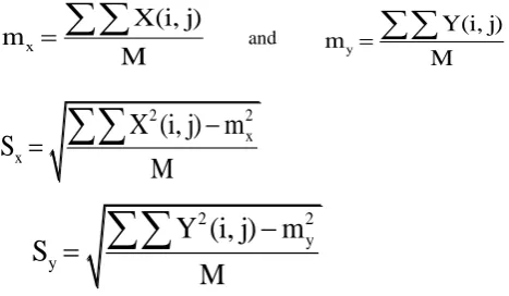
In normalized form, Γ is the sample correlation coefficient

between the entries of the two matrices. If m

x

and m

y

denote the

sample means and S

x

and S

y

denote the sample standard

deviations of the entries of matrices

X

and

Y,

the normalized Γ

statistics is

n 1 n

x y

i 1 j i 1

x y

[X(i, j)

m ][Y(i, j)

m ]

M S S

   



_

_











  















 

Where M =n(n-1)/2 is the number of entries in the double sum

and the moments are given by

x

X(i, j)

m

M





and

y

Y(i, j)

m

M





2 2 x x

X (i, j) m

S

M







2

2

y

y

Y (i, j) m

S

M







All sums are over the set {(i,j): 1



i



n-1, i+1



j



n}. The Γ

statistics measures the degree of linear correspondence between

the entries of

X

and

Y.

The large absolute value of Γ suggests

that the two matrices agree with each other. The normalized Γ is

always between -1 and 1.

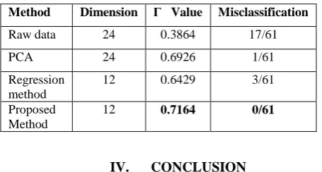
Table 3 gives summary of the results obtained from various

experiments on this data. The proposed method shows high Γ

value with no classification error.

Method

Dimension

Association

Disassoci

ation

CTI

Raw data

24

0.351

0.477

0.828

PCA

24

0.242

0.910

1.152

Regression

method

12

0.815

0.250

1.065

Proposed

Method

12

0.1687

1.0358

1.204

5

Partition

Cities

Cluster 1

Athens, Hongkong, Lisbon,

London, Madrid, Newyork, Paris,

Rome, San Francisco, Tokyo

Cluster 2

Bahrain, Bombay, Cairo, Calcutta,

Colombo, Dubai, Kuala Lumpur,

Madras, Manila, Mexico, New

Delhi, Singapore

Cluster 3

Frankfurt, Seoul, Zurich

Cluster 4

Amsterdam, Copenhagen, Geneva,

Moscow, Munich, Stockholm,

Toronto, Vienna

Table 3: Comparison of Γ value of various methods for

Corn Soybean data

IV.

CONCLUSION

In this chapter, a novel method of reducing the feature set

into symbolic features and a novel method of measuring

proximity between samples expressed as intervals is

introduced.

The

proposed

model

achieves

better

performance in terms of CTI for City Temperature data and

Hubert Γ statistics in case of CORN SOYBEAN data.

V.

REFERENCES

[1] Betrand P ,Goupil F, Descriptive statistics for symbolic

data, analysis of symbolic data, Bock H.H and Diday

E(eds) Springer, 1999.

[2] Bock H.H , Diday E, Analysis of symbolic data,

Springer Verlag, 2000.

[3] De Carvalho.F.A.T, Souza R, New metrics for

constrained Boolean symbolic objects, Proc of KESDA98,

Eurostat, Luxemberg 1998.

[4] Diday E, An introduction to symbolic data analysis,

Tutorial of 4th Conf of IFCS, Paris, 1993.

[5] Gowda.K.C ,Diday.E, Symbolic clustering using a new

dissimilarity measure, Pattern Recognition, Vol 24, no.6,

pp 567-578, 1991.

[6] Gowda.K.C ,Diday.E, Symbolic clustering using a new

similarity measure, IEEE Trans on SMC, Vol 22, No.2,

Mar/April 1992.

[7] Ichino.M, Yaguchi.H, Generalized Minkowsi’s metrics

for mixed feature type data analysis, IEEE Trans on SMC,

24(4), pp 698-708, 1994.

[8] Jain A.K, Dubes.R.C, Algorithm for clustering data,

Prentice Hall, pp 23-46, 143-220, 1988.

[9] Jolliffe.I.T, “Principal Component Analysis” Springer

Verlag, NY, 1986.

[10]

Lalitha Rangarajan ,Nagabhusha.P, Dimensionality

reduction of multi dimensional temporal data through

regression, Pattern Recognition Letters, Vol 25/8,

pp.899-910, 2004.

[11]Michalski R.S, Diday E, Stepp R.E, A recent advance

in data analysis: Clustering objects into classes

characterized

by

conjunctive

concepts,

Pattern

Recognition, vol.1, pp33-56, 1981.

[12]Nagabhushan P, Gowda K C and Diday E,

Dimensionality reduction of symbolic data, Pattern

Recognition Letters, Vol 16, pp 219-213, 1995.

[13] Nagabhushan P, An efficient method for classifying

remotely sensed data, incorporating Dimensionality

Reduction, PhD Thesis, University of Mysore, Mysore,

1988.

VI.

ABOUT

THE

AUTHORS

Veerabhadrappa obtained his M.Sc. and Ph.D, degrees in

Computer Science and Technology from the University of

Mysore, India, respectively in the years 1989 and 2011.

Currently he is working as Associate Professor and Head of

the department of Computer Science, University College,

Mangalore, India. He has authored 12 peer-reviewed

papers in journals and conferences. He is the reviewer of

the Journal of Neurocomputing and International Journal of

Computer Applications (IJCA). His area of research covers

dimensionality reduction, face/object recognition and

symbolic data analysis.

Dr. Lalitha Rangarajan is currently a Professor in

Department of Computer Science, University of Mysore,

India. She has two master degrees one in Mathematics from

Madras University, India and the other in Industrial

Engineering (specialization: Operations Research) from

Purdue University, USA. She has taught mathematics for

five years in India soon after the completion of masters in

mathematics. She is associated with the Department of

Studies in Computer Science, University of Mysore, soon

after completion of masters at Purdue University. She

completed her doctorate in Computer Science in 2004 and

since then doing research in the areas of image processing,

retrieval of images, bioinformatics and pattern recognition.

She has more than 40 publications in reputed conferences

and journals to her credit.

Method

Dimension

Γ Value Misclassification

Raw data

24

0.3864

17/61

PCA

24

0.6926

1/61

Regression

method

12

0.6429

3/61

Proposed

Method

Appendix A: Minimum and maximum temperature of 39 cities

Sample No.

Cities

Jan Feb Mar Apr May Jun Jul Aug Sept Oct Nov Dec 1 _Amsterdam

[ -4, 4] [ -5, 3] [ 2, 12] [ 5, 15] [ 7, 17] [ 10, 20] [ 10, 20] [ 12, 23] [ 10, 20] [ 5, 15] [ 1, 10] [ -1, 4] 2 _{Athens [ 6, 12] [ 6, 12] [ 8, 16] [ 11, 19] [ 16, 25] [ 19, 29] [ 22, 32] [ 22, 32] [ 19, 28] [ 16, 23] [ 11, 18] [ 8, 14]} 3 _{Bahrain [ 13, 19] [ 14, 19] [ 17, 23] [ 21, 27] [ 25, 32] [ 28, 34] [ 29, 36] [ 30, 36] [ 28, 34] [ 24, 31] [ 20, 26] [ 15, 21]} 4 _{Bombay [ 19, 28] [ 19, 28] [ 22, 30] [ 24, 32] [ 27, 33] [ 26, 32] [ 25, 30] [ 25, 30] [ 24, 30] [ 24, 32] [ 23, 32] [ 20, 30]} 5 _{Cairo [ 8, 20] [ 9, 22] [ 11, 25] [ 14, 29] [ 17, 33] [ 20, 35] [ 22, 36] [ 22, 35] [ 20, 33] [ 18, 31] [ 14, 26] [ 10, 20]} 6 _{Calcutta [ 13, 27] [ 16, 29] [ 21, 34] [ 24, 36] [ 26, 36] [ 26, 33] [ 26, 32] [ 26, 32] [ 26, 32] [ 24, 32] [ 18, 29] [ 13, 26]} 7 _{Colombo [ 22, 30] [ 22, 30] [ 23, 31] [ 24, 31] [ 25, 31] [ 25, 30] [ 25, 29] [ 25, 29] [ 25, 30] [ 24, 29] [ 23, 29] [ 22, 30]} 8 _{Copenhagen [ -2, 2] [ -3, 2] [ -1, 5] [ 3, 10] [ 8, 16] [ 11, 20] [ 14, 22] [ 14, 21] [ 11, 18] [ 7, 12] [ 3, 7] [ 1, 4]} 9 _{Dubai [ 13, 23] [ 14, 24] [ 17, 28] [ 19, 31] [ 22, 34] [ 25, 36] [ 28, 39] [ 28, 39] [ 25, 37] [ 21, 34] [ 17, 30] [ 14, 26]} 10 _{Frankfurt [-10, 9] [ -8, 10] [ -4, 17] [ 0, 24] [ 3, 27] [ 7, 30] [ 8, 32] [ 8, 31] [ 5, 27] [ 0, 22] [ -3, 14] [ -8, 10]} 11 _{Geneva [ -3, 5] [ -6, 6] [ 3, 9] [ 7, 13] [ 10, 17] [ 15, 17] [ 16, 24] [ 16, 23] [ 11, 19] [ 6, 13] [ 3, 8] [ -2, 6]} 12 _{Hong Kong}

Appendix B: Corn dataset

Sample No.

June 11, 1979 June 29, 1979 July 16, 1979 August 30, 1979 F1 F2 F3 F4 F5 F6 F1 F2 F3 F4 F5 F6 F1 F2 F3 F4 F5 F6 F1 F2 F3 F4 F5 F6

Appendix B: Soybean dataset

Sample No.

June 11, 1979 June 29, 1979 July 16, 1979 August 30, 1979

F1 F2 F3 F4 F5 F6 F1 F2 F3 F4 F5 F6 F1 F2 F3 F4 F5 F6 F1 F2 F3 F4 F5 F6