Registration of Multimodal Brain Images Using Modified Adaptive Polar Transform

(1)

Registration of Multimodal Brain Images Using

Modified Adaptive Polar Transform

D.Sasikala, R.Neelaveni

Abstract-- Image registration has great significance in medicine, astrophotography and satellite imaging, so a lot of techniques have been developed within its perspective of one or the other discipline. This paper presents a method for medical image registration of multimodal brain images using Modified Adaptive Polar Transform (MAPT). This algorithm can be used to register images of the same or different modalities. The performance of the Adaptive Polar Transform (APT) with the proposed technique is examined. The proposed scheme not only reduces the source of errors and also reduces the time for registration of brain images. The analysis presented for the medical image registration using Modified Adaptive Polar Transform (MAPT) and APT proves that MAPT performs better than APT technique.

Index Term-- Adaptive Polar Transform; Correlation Coefficient, Gabor wavelet transform; Modified Adaptive Polar Transform; Modified Gabor wavelet transform; Mutual Information.

1. INTRODUCTION

Image registration is the method of superimposing images (two or more) of the similar view captured at various times, from different perspectives, and/or by different sensors. The registration geometrically aligns two images (the model and sensed images). These approaches are classified based on their nature (area based and feature-based) and have four fundamental steps: (i) feature detection, (ii) feature matching, (iii) mapping function design, and (iv) image transformation and sampling.

The up to date differences between images are initiated due to different imaging conditions.

Image registration is an essential accomplishment in all image analysis tasks in which the ultimate information is realized from grouping of a range of data sources like in image fusion, change detection, and multichannel image restoration. Normally, registration is required in medicine (combining CT and / or MRI data to obtain additional complete information about the patient, monitoring tumour growth, treatment verification, evaluation of the patient’s data with anatomical atlases), and in computer vision (target localization, automatic quality control).

Many techniques of the image registration have been proposed previously. Medha V. Wyawahare et al.[1]

D.Sasikala is with Bannari Amman Institute of Technology, Sathyamangalam, Tamil Nadu-638401. as Assistant Professor in Department of Computer Science and Engineering (Mobile number 9790597069 and Email address :

[email protected]

R.Neelaveni is with PSG College of Technology, Coimbatore, Tamil Nadu -641004. as Assistant Professor in Department of

Electrical and Electronics Engineering (Email address : [email protected])

proposed Image registration as a vital problem in medical imaging with many applications in clinical diagnosis (Diagnosis of cardiac, retinal, pelvic, renal, abdomen, liver, tissue etc disorders). Ashok Veeraraghavan et al. [2] presented an approach for comparing two chains of deforming shapes by both parametric models like the autoregressive model and autoregressive moving average model and nonparametric methods based on Dynamic Time Warping. Kendall's definition of shape is used for feature extraction. E.D. Castro and C. Morandi [3] placed steps for the new technique, based on the Fourier-Mellin transform that rapidly identify global affine transformations applied to tabular document images, and to correct those. L. G. Brown [4] stated registration as an intermediate step. J. P. Lewis [5] described image registration as cross correlation that is efficiently executed in the transform domain and its normalized form is preferred for feature matching applications. S. Zokai and G.Wolberg [6] gave an idea about registration of multi resolution and multisensory images as a challenging problem inthe research area of remote sensing. They proposed a new method for automatic affine imageregistration based on local descriptors, called automatic image registration by local descriptors (AIRLD). V. J. Traver et al [7], H. Araujo et al [8] and H. S. Stone et al [9] discussed about the log polar transform technique for image registration. D. Lowe [11] presented a technique for extracting distinctive invariant features from images that can be used to achieve reliable matching among different views of an object or scene. J. B. Antoine Maintz et al. [10, 12] presented a review of recent publications concerning medical image registration techniques.

In probability theory and information theory, Mutual Information [13, 14] (sometimes known as transinformation) between two discrete random variables is termed as the amount of information shared between the two random variables. It is a dimensionless quantity with units of bits and can be the reduction in uncertainty. High Mutual Information (MI) [13, 14] indicates a large reduction in uncertainty; low MI indicates a small reduction; and zero MI between two random variables means the variables are independent.

Mutual Information

(1)

(2)

p(x,y) - Joint probability distribution function of X

and Y.

p1(x) and p2(y) - Marginal probability distribution functions of X and Y respectively.

Correlation Coefficient

(2)

- Two new images that differ from each other by

translation and rotation only. t ,s - Shifting parameters between the two images.

- Rotation angle.

- Average structure value of the pixels in the overlapping parts of images

respectively.

The Correlation Coefficient CC [14, 15], is a measure of how well the predicted values from a forecast model “fit” with the real-life-data. If there is no relationship between the predicted values and actual values the CC is very low. As the strength of the relationship between the predicted values and actual values increases, so does the CC. Thus higher CC is better.

2. IMAGE REGISTRATION APPROACH USING ADAPTIVE POLAR TRANSFORM (APT)

2.1. Localization

In APT, the translation parameter between the two images is determined. Fourier phase correlation is used to fix the translation before calculating the log-polar matching [7, 8] in the frequency domain. However, a study in [9, 13] showed the aliasing problem by using the phase magnitude of Fast Fourier Transform (FFT) to pick up the translation (of the centre point). Zokai et al. [6] used a multi resolution imaging technique to remove the computation cost of translation recovery by searching from the coarsest to the finest level. This performs well only if target image contains enough low frequency information and that component are not deformed by noise. A new method based on a reduced set of feature points is established to pace the search procedure. The search is lessened from every pixel of the target image to a set of feature points only. These are got by applying Gabor transform to every pixel and selecting those pixels that generate high energy in the wavelet domain.

Fig. 1. Feature point extraction and localization procedure for Transaxial T1 MR JPEG image of size 718 kB with resolution 1044 x 2219 pixels. First, feature points are extracted from both the model image and the target image of a single modality, either CT or

MRI. and are sets of

feature points in the model image and in the target image, respectively. The superscription and M and T denote the model image and the target image, and nM and nT are the number of feature points in the model image and the number of feature points in the target image, respectively. To crop the model image out of the image, automatically one of the feature points is selected in the model image e as a centre point for APT and chooses the size of the radius for the transformation Rmax that adequately covers the model image to compute APT RM_{and Θ}M_{the projections of Adaptive Polar} Transform (APT), RM_{and Θ}M_{. On the left is the model image} (From Fig 1.Brain Image with the size 1044 x 2219 pixels) with 166 feature points identified. The model image is created by selecting one of the feature points in the model image as the origin, and is cropped to a circular image patch that covers the area Rmax desired to be registered to the target image. On the right is the target image (From Fig 1. Brain Image that is scaled by 0.7 and rotated by 30 degrees, the size of the image is 730x1553 pixels) with 180 feature points identified. To obtain the translation between the model image and the target image, the corresponding feature point is located in the target image. As shown in Fig 1, the search space is limited to only a set of feature points in the target image, which is approximately 0.2% of the total number of pixels in the target image in this example. Hence, the search space is much smaller than that of the exhaustive search strategy.

2.2. APT Matching

After extracting feature points in the model image and selecting one feature point as the centre point for computing the projections RM_{and Θ}M_{using the APT} approach, the next step is to find the related feature point in the target image and obtain both the scale and the rotation parameters between the two images of the same modalities. Given a set of feature points in the target image and the radius size of the APT transformation Rmax to be identical as for computing the projections RM_{and Θ}M_{, each feature point is} applied in the target image as a centre point for computing

APT creating the set of candidate

projections and . By

matching and with each member in the sets of projections RM and ΘM_{, respectively, the translation, scale, and rotation}

new new

I I1 , 2

 ) , ( ), , ( ₂

1 x y I x y

Inew new

) , ( , ) , ( ₂

1 x y I x y

Inew new

               

x y x y

(3)

parameters are obtained concurrently. The matching results have three dimensions: the scale parameter, the rotation parameter, and the distance coefficient. The translation parameter is the offset involving the locations of to the feature point in the target image that defers the lowest distance coefficient. For a given feature point in the target image, IM_, _, _and _{are denoted as the model image,} the image area that is cropped from the target image to be matched with the model image, the projection on the radius coordinate, and the projection on the angular coordinate, respectively. Then the scale change in the Cartesian coordinates reflects as variable-scalene of the projection, and the rotation change reflects as shifting in the projection. Therefore, the new matching mechanisms are put forward to obtain both the scale and the rotation parameters. The mathematical expression of image that is scaled and rotated version of image IM _is

(3)

In the polar domain, equation (3) can be expressed as

(4)

Where az and θz are the scale and the rotation parameters, respectively. As shown in equations (3) and (4), the scale parameter az, in the Cartesian coordinates appears as scaling with the same value in the radius direction of the polar transformed image. For the case of adaptive sampling in APT, the outcome of scaling is seen in the Cartesian to APT mapping remains similar to that of the polar transform mapping. Except for APT, the number of samples in the angular direction can vary (adaptive).To calculate the 1-D projection in the radius direction R(i), multiplication variable Ωi is initiated to compensate the effect of adaptive sampling in the angular direction. As a result, the 1-D projection R of APT is an approximation to that of the polar transformed image. From previous works,

(5)

and

(6)

is obtained. is calculated in terms of RM _{as follows:}

(7)

(8)

Thus, the variable-scale az is a global and uniform scale for the 1-D projection R curve. As shown in Fig. 2(a) and (c), the projections Θ of the scaled images in the Cartesian is a little altered when compared with that of the original image. This is because the areas enclosed during the APT transformations are unlike as a result of the scaling. Hence, in order to precisely obtain the shifting parameter involving the two projections ΘM and ΘT _{and, the variable-scale parameter az involving the two} projections RM _and _{must be obtained first.}

(a)Find Scale Parameter: Amongst the several ways of getting the scale parameter from the projections depending on the prerequisites of the application in terms of the computational cost, accuracy, image types and environments, two effective algorithms are initiated.

Algorithm 1: Fourier Method: Based on the property of

Fourier transform, given a Fourier transform of signal as, the Fourier transform of the scaled signal x (t) can be expressed as

(9)

(10)

Similar to the polar transform, the projection calculated from image that is the scaled version of image IM_{with the} scale parameter az will also be the scaled version of the projection with the same scale parameter az. From equations (9) and (10), given the Fourier transform of the projection R(.) as Г(.), the scale parameter can be obtained by

(11)

(12)

This Fourier technique executes well only when the scale parameter is small. Large scale parameter defers the aliasing problem. Hence, this algorithm is apt for applications that involve fast and accurate image registration while the scale parameter involving the two images is expected to be small, such as medical image registration.

Algorithm 2: Logarithm Method: The second algorithm

applies the scale invariant property of the logarithm function. First, the logarithm function is applied to the projection R and the output is then quantized to maintain the original dimension of the projection. The mathematical expression of the operation is as follows:

(4)

The parameter LR(.) shows the logarithmic of the projection R. Given image a scaled and rotated version of image IM_{, the scale parameter az}_{involving the two images} would shows translation in the logarithm domain L

(14)

To find the displacement d, where d=log az, such

that , the correlation function can be

assessed between the two logarithmic of projections

(15)

This algorithm defers high accuracy and fast matching in the general condition.

(b) Find Rotation Parameter: After the scale parameter is obtained, the next step is to find the rotation parameter θz. For the same sampling radius, Rmax, the larger the image (az>>1), the smaller the area of the scene is covered in the sampling procedure. As a result, the magnitude of the projections Θ between the two images could be slightly altered. This detail is illustrated in Fig. 2(a) and (c). As a result, to precisely acquire the rotation parameter θz, must be adapted according to the scale parameter az: the equations (16) and (17) are examined. Both projections are then resampled to be equal in length. The rotation parameter can be found by evaluating the

correlation function )

(16)

(17)

(c)Find Distance Coefficient: The final and important

component resulting from APT matching is the distance coefficient, denoted as εz, which show how large is the variation that involves the two images. The distance coefficient εz between the model image IM_{and the target} image can be worked out from the Euclidean distance between the projections

(18)

For the intended image registration approach, one feature point is searched in the target image that corresponds with the feature point in the model image. Such feature point is the point that yields the lowest distance coefficient. The projections RM_and _{are not used for computing the distance} coefficient εz because the dimension of projections that can be utilized in the computation varies depending on the scaling

parameter az. As a result, only the projections and are used in the computation.

2.3. Image Comparison

With the advantages of APT, a quick and simple image comparison method is put forward that can effectively and automatically position the altered area or the area where the registered image pair differs without further computational cost. Since the scale difference in the Cartesian coordinates between the model image and the target image yields different area coverage in the transformation process, the dimension of the projection R for comparing the two images needs to be altered accordingly. Given the scale and the rotation parameters between the model image and the target image as akr _{and θk}’_{, respectively, the altered area is found as a set of} pixels (X,Y) in the Cartesian coordinates, where X=x1,….,xt, Y=y1,…,yt, and parameter is the number of pixels in the altered area as follows:

(19)

(20)

The location of is denoted in the Cartesian

coordinates as (cx ,cy). For , the set of image

pixels is computed in the altered area (X,Y) as follows:

(21)

(22)

The image comparison to find altered area between two images can be done by any registration algorithm, if image registration can be achieved. The recommended method is robust in the sense that the image with altered area even in the centre can still be registered plus the condition of the Log Polar Transform (LPT advantages) in scale and rotating invariant. In addition, the altered area can be recognized

(23)

(5)

without extra computational cost. For most registration algorithms, to compare two images involving the 2D geometric transformation, additional computations are essential as post processes such as image alignment; transform both images to the same coordinates prior to the comparison, and image

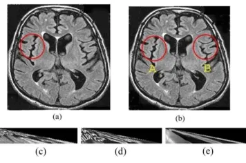
Fig. 2. Example of the proposed image registration approach (a) model image where the model image is the area inside the circular line, (b) two candidates are chosen as examples using two feature points A and B of the target image, (c) APT of the model image, (d) and (e) APTs of the target image where the centre points of the transformation are feature points A and B, respectively.

normalization. For the proposed image registration approach, since both the model image and the target image are already transformed to the projections of the APT domain, image comparison can be performed directly and simultaneously while obtaining scale and rotation parameters.

3. MODIFIED ADAPTIVE POLAR TRANSFORMATION

(MAPT)

The registration of images using Modified Adaptive Polar Transform (MAPT) yields accuracy with much less computational load when compared to Adaptive Polar Transform (APT). It can also register images that are altered and occluded accurately because it gives importance to the entire image equally.

While using Algorithm I: Fourier Method of finding the Scale Parameter a multiscale transform of a signal U may be defined as

(25)

where a > 0 is the scale parameter, b is the time (or position) parameter, and denotes the analyzing function. Different analyzing functions may be taken up with this general transform. In particular, the analyzing function of the Short-Time Fourier Transforms (STFT) using a Gaussian window (also known as Gabor transform).

(26)

where . The analyzing function in the wavelet transform using a Gabor wavelet (also called a Morletwavelet).

(27)

Where ω0 is the basic frequency of ψGWT. The Gabor and the Gabor-wavelet transforms are commonly implemented to do local frequency analysis because they are well localized in the time and frequency domains. The Gabor and Gabor-wavelet transforms analyze signals at different frequencies and scales but in a dependent way, i.e., the frequency content range depends on the working scale. This is not desirable for image analysis as the coding regions are characterized by a fixed periodicity that may occur at different scales. Neither of these transforms is suitable for such task. Therefore, the Modified Gabor Wavelet Transform (MGWT) is defined as a function of b and a as

(28)

(29)

For the evaluation of the algorithm, 6 such sets of MR and CT image pairs are considered. Table I show the summary of all the results when a single ordering is taken into account using APT and MAPT in terms of MI. X, Y represents the translated points, Ө represents the rotation angle, CC represents Correlation Coefficient, and MI represents Mutual Information [13, 14]. Fig 23.shows the performance comparison of APT and MAPT in terms of MI. Table II represents the summary of all results using APT and MAPT in terms of CC. Fig 24. shows the performance comparison of APT and MAPT in terms of CC. Table III indicates the Elapsed time for registering image using APT and MAPT. Fig 25.represents the comparison elapsed time of APT and MAPT.

(i) Axial 427 x 442 - 71k - jpg CT & Axial 427 x 442 - 62k – jpg MRIT2 – APT

Fig. 3. Registered Image obtained using APT

(ii) Axial 427 x 442 - 71k - jpg CT & Axial 427 x 442 - 62k – jpg MRIT2 – MAPT

Fig. 4. Registered Image obtained using MAPT

(6)

(iv) Axial 427 x 442 - 71k - jpg CT & Axial 427 x 442 - 62k – jpg MRIT2 – MAPT

(v) Frontal 400 x 400 - 11k – jpg MRIT1 & Frontal 400 x 400 - 18k – jpg MRIT1 –APT

(vi) Frontal 400 x 400 - 11k – jpg MRIT1 & Frontal 400 x 400 - 18k – jpg MRIT1 –MAPT

(vii) Frontal 400 x 400 - 18k – jpg MRIT1 & Frontal 400 x 400 - 11k – jpg MRIT1 -APT

(viii) Frontal 400 x 400 - 18k – jpg MRIT1 & Frontal 400 x 400 - 11k – jpg MRIT1 -MAPT

(ix) Frontal 400 x 400 - 11k – jpg MRIT1 & Sagittal 400 x 400 - 24k – jpg MRIT1- APT

(x) Frontal 400 x 400 - 11k – jpg MRIT1 & Sagittal 400 x 400 - 24k – jpg MRIT1- MAPT

(xi) Sagittal 400 x 400 - 24k – jpg MRIT1 & Frontal 400 x 400 - 11k – jpg MRIT1- APT

(xii) Sagittal 400 x 400 - 24k – jpg MRIT1 & Frontal 400 x 400 - 11k – jpg MRIT1- MAPT

(xiii) Frontal 400 x 400 - 18k – jpg MRIT1 & Sagittal 400 x 400 - 24k – jpg MRIT1 - APT

(xiv) Frontal 400 x 400 - 18k – jpg MRIT1 & Sagittal 400 x 400 - 24k – jpg MRIT1 -MAPT

(7)

(xvi) Sagittal 400 x 400 - 24k – jpg MRIT1 & Frontal 400 x 400 - 18k – jpg MRIT1-APT

(xvii) Axial 350 x 350 - 21k – jpg MRIT2 & Frontal 350 x 350 - 24k - jpg MRIT2- APT

(xviii) Axial 350 x 350 - 21k – jpg MRIT2 & Frontal 350 x 350 - 24k - jpg MRIT2- MAPT

(xix) Frontal 350 x 350 - 24k - jpg MRIT2 & Axial 350 x 350 - 21k – jpg MRIT2- APT

(xx) Frontal 350 x 350 - 24k - jpg MRIT2 & Axial 350 x 350 - 21k – jpg MRIT2- APT

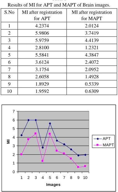
Table I

Results of MI for APT and MAPT of Brain images. S.No MI after registration

for APT

MI after registration for MAPT

1 4.2374 2.0124

2 5.9806 3.7419

3 5.9759 4.4139

4 2.8100 1.2321

5 5.5841 4.3847

6 3.6124 2.4072

7 3.1754 2.0952

8 2.6058 1.4928

9 1.8929 0.5339

10 1.9592 0.6309

0 1 2 3 4 5 6 7

1 2 3 4 5 6 7 8 9 10 Images

MI

APT MAPT

Fig. 23. Comparison of APT and MAPT using MI.

From the analysis using MI it shows that the performance of APT is better than MAPT.

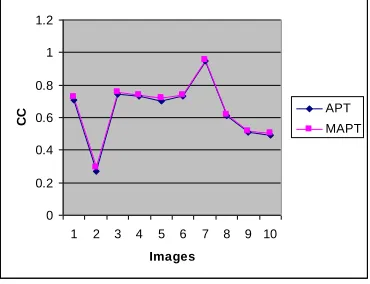
Table II

Results of CC for APT and MAPT of Brain images. S.No CC after registration

for APT

CC after registration for MAPT

1 0.7089 0.7246

2 0.2678 0.2928

3 0.7410 0.7576

4 0.7319 0.7392

5 0.6992 0.7184

6 0.7349 0.7409

7 0.9502 0.9537

8 0.6103 0.6187

9 0.5096 0.5162

(8)

0 0.2 0.4 0.6 0.8 1 1.2

1 2 3 4 5 6 7 8 9 10

Images

CC

APT MAPT

Fig. 24. Comparison of APT and MAPT using CC.

From the analysis using CC it shows that the performance of MAPT is better than APT.

Table III

Elapsed time for registration using APT and MAPT of Brain images. S.No Elapsed Time

in seconds for APT

Elapsed Time in seconds for MAPT

1 3.265 1.516

2 2.766 1.672

3 1.719 0.953

4 1.640 0.953

5 1.656 0.937

6 1.672 0.938

7 1.641 0.937

8 1.641 0.938

9 1.625 1.046

10 1.594 1.046

0 0.5 1 1.5 2 2.5 3 3.5

1 2 3 4 5 6 7 8 9 10

Images

E

la

p

s

e

d

T

im

e

i

n

S

e

c

o

n

d

s

APT MAPT

Fig. 25. Comparison of APT and MAPT using Elapsed Time for Registration.

From the analysis using Elapsed Time for registration it shows that the performance of MAPT is better than APT.

For the evaluation of the algorithm, 10 such sets of CT and MRI image pairs were used. Table I, Table II and Table III. shows the registration results of brain images taken into account using GWT in APT and MGWT in MAPT. Fig 24, and Fig 25 reveals that the performance of MAPT is better

than APT. Fig 23 reveals that the performance of APT is better than APT. Hence any other better technique is to be implemented to rectify the problem for registration of images to improve MI.

4. CONCLUSION

A series of simulations was performed using medical images. The tests were performed using same images of different sizes. Registration of Multimodality brain images using MRI- T1, T2 and CT scan images are studied and were examined with regard to accuracy, robustness with respect to starting estimate. Finally, a set of CT medical images are used that depict the head of the same patient. In order to remove the background parts and the head outline, the original images are cropped, creating sub-images of lesser dimensions. The experimental results revealed the fact that the application of MAPT performs well in image registration. The future work concentrates on improving the mutual information for multimodal images using MAPT and also to further improve the results by using some other transforms that use correlation coefficients.

REFERENCES

[1] Medha V. Wyawahare, Dr. Pradeep M. Patil, and Hemant K. Abhyankar, “Image Registration Techniques: An overview”, International Journal of Signal Processing, Image Processing and Pattern Recognition Vol. 2, No.3, pp.1-5, September 2009.

[2] Ashok Veeraraghavan, “Matching Shape Sequences in Video with Applications in Human Movement Analysis” , IEEE Transactions on Pattern Analysis and Machine Intelligence, vol. 27 no. 12, pp. 1896-1909, December 2005

[3] E.D. Castro, C. Morandi, “Registration of translated and rotated images using finite Fourier transform", IEEE Transactions on Pattern Analysis and Machine Intelligence, vol.9, pp. 700–703, (1987).

[4] L. G. Brown, “A survey of image registration techniques,” ACM Comput. Surv., vol. 24, no. 4, pp. 325–376, Dec. 1992.

[5] J. P. Lewis, “Fast normalized cross-correlation,” in Proc. Vision Interface, May 1995, pp. 120–123.

[6] S. Zokai and G.Wolberg, “Image registration using log-polar mappings for recovery of large-scale similarity and projective transformations,” IEEE Transaction in Image Processing, vol. 14, no. 10, pp. 1422–1434, Oct. 2005.

[7] V. J. Traver and F. Pla, “Dealing with 2D translation estimation in log polar imagery,” Image Visual Computation, vol. 21, no. 2, pp. 145–160, Feb. 2003.

[8] H. Araujo and J. M. Dias, “An introduction to the log-polar mapping,” in Proc. 2nd Workshop Cybernetic Vision, Dec. 1996, pp. 139–144. [9] H. S. Stone, B. Tao, and M. McGuire, “Analysis of image registration

noise due to rotationally dependent aliasing,” J. Vis. Communication and Image Representation vol. 14, no. 2, pp. 114–135, Jun. 2003. [10]J. B. A. Maintz and M. A. Viergever, “A survey of medical image

registration,” Medical Image Analysis, vol. 2, no. 1, pp. 1–36, Mar. 1998.

[11]D. Lowe, “Distinctive image features from scale-invariant keypoints,” Int. J. Comput. Vis., vol. 60, no. 2, pp. 91–110, Nov. 2004.

[12]J. B. Antoine Maintz_ and Max A. Viergever,” A Survey of Medical Image Registration,” October 16, 1997

[13]I. Grosse, H. Herzel, S.V. Buldyrev, and H.E. Stanley, “Species Independence of Mutual Information in Coding and Noncoding DNA,” Physical Rev. E, vol. 61, no. 5, pp. 5624-5629, 2000.

(9)

[15]W. Li, T.G. Marr, and K. Kaneko, “Understanding Long-Range Correlations in DNA Sequences,” Physica D, vol. 75, pp. 392-416,1994.

D.Sasikala is presently working as Assistant Professor, Department of CSE, Bannari Amman Institute of Technology, Sathyamangalam. She received B.E.( CSE) from Coimbatore Institute of Technology, Coimbatore and M.E. (CSE) from Manonmaniam Sundaranar University, Tirunelveli. She is now pursuing Phd in Image Processing. She has 11.5 years of teaching experience and has guided several UG and PG projects. She is a life member of ISTE. Her areas of interests are Image Processing, System Software, Artificial Intelligence, Compiler Design.