Vibrations of a Non-Linear Dynamical System with Time Varying Stiffness Subjected to Multi- Excitation Forces

(1)

International Journal of Basic & Applied Sciences IJBAS-IJENS Vol:13 No:04 79

Vibrations of a Non-Linear Dynamical System with

Time Varying Stiffness Subjected to Multi-

Excitation Forces

Y. A. Amer

*

, E. El emam. Ahmed

Abstract-- Vibration and dynamic chaos are undesired

phenomenon in structure. The system of single degree of freedom of a cantilever skew of aluminum plate are introduced using quadratic and cubic non-linearities with time varying stiffness are considered and studied. The multiple time scale perturbation technique is applied. An approximate solution is derived up to third order approximation. The stability of the system investigated applying both frequency response functions (FRFs) and phase-plane methods. The effects of

different parameters are studied numerically.

Index Term--Chaotic, Perturbation method, Response curves,

Stability.

I. INTRODUCTION

Vibrations are the cause of discomfort, disturbance, damage, and sometimes destruction of machines and structures. It must be reduced or controlled or eliminated. Arafat and Nayfeh [1] studied the motion of shallow suspended cables with primary resonance excitation. The method of multiple scales is applied to study nonlinear response of this suspended cables and its stability and the dynamic solutions. Zheng, Ko and Ni [2] considered the super-harmonics and internal resonance of a suspended cable with almost commensurable natural frequencies. Zhang and Tang [3] investigated the chaotic dynamics and global bifurcations of the suspended inclined cable under combined parametric and external excitations. Amer and Sayed [4], studied the response of one-degree freedom, non-linear system under multi-parametric and external excitation forces simulating the vibration of the cantilever beam. Variation of some parameters leads to multi-valued amplitudes and hence to jump phenomena. Sayed et al. [5], investigated the non-linear dynamics of a two degree-of freedom vibration system including quadratic and cubic non-linearities subjected to external and parametric excitation forces. The stability of the system is investigated using both frequency response curves and phase-plane trajectories. The effects of different parameters of the system are studied numerically. Cheng-Tang Lee et al. [6] demonstrated that a dynamic vibration absorber system can be used to reduce speed. fluctuations in rotating machinery active constrained layer damping (ACLD) has been Y. A.

Amer is with Department of Mathematics, Faculty of Science, Zagazig University, Egypt.

(e-mail: [email protected])

*Corresponding author

E. El emam. Ahmedis with Department of Basic Science, Higher Technological Institute, 10th_{of Ramadan City, Egypt}

.( e-mail: [email protected])

successfully utilized as effective means damping out the vibration of various flexible structures [7-9]. When the system is excited at a frequency near the higher natural frequency, the structure responds at the excitation frequency and the amplitude of the response increases linearly with the excitation amplitude. How ever, when the high frequency modal amplitude reaches a critical

(2)

International Journal of Basic & Applied Sciences IJBAS-IJENS Vol:13 No:04 80 Hamed [20] studied the response of a

two-degree-of-freedom System with quadratic coupling under parametric and harmonic excitations. The method of multiple scale perturbation technique is applied to solve the non-linear differential equations

and obtain approximate solutions up to and including the second-order approximations.

In this work the system of single degree of freedom of a cantilever skew of aluminum plate are introduced using quadratic and cubic non-linearities with time varying stiffness are considered and studied. The multiple time scale

perturbation technique is applied. An approximate solution is derived up to third order approximation. The stability of the system investigated applying both frequency response functions (FRFs) and phase-plane methods. The effects of different parameters are studied numerically.

II. MATHMARICAL MODELING

The investigated equation is the modified non-linear differential equation describing the vibration of an aircraft

wing which is given by:

(1) where u represents displacement of the vibration, damping

coefficient,

 

,

₁ and



₂ are nonlinear stiffness coefficients

,

S

is the time varying stiffness,

F

_j are the amplitudes of excitation,



_j are the excitation frequencies.

A. Perturbation analysis

We seek a first-order approximate solution of equation (1) by using the method of multiple scales in the form

1

0

,

(

)

k

( , )

k o

k

t

u

 







u T T



(2)

where

2

1 2 ...,

, 0,1, 2,...

o

i i

d

D D D

dt

D i

T

     



 



where



is small dimensionless parameter used for book-keeping only ;

T

_o



t

and

T

₁

 

t

are the fast and slow time scales respectively . Substituting equation (2) into equation (1) and equating coefficients of like powers of



, we obtain the following set of ordinary differential equations

2 2

(

D

_o

 

)

u

_o



0

(3(

2 2 2

1 1

3

1 2

1

(D

)

2

2 (

cos

)

cos

o o o o o o

N

o o j j o

i

u

D D u

D u

u

ST u

F

T



 

 

 

 

   







(4)

2 2 2

2 1 1 1 1

2

1 1 1 2 1

(

)

2

2 (

) 2

3(

cos

)

o o o o

D

u

D D u

D u

u u

ST u u

 

 



 



 

   

(5)

2 2 2

3 1 2 1 1 2

2 2

1 1 1 2 1 2 2

(

)

2

2 (

)

(

2 ) 3(

cos

)(

o o o

o o

D

u

D D u

D u

u

u u

ST

u u

 

 



 



 



   

2 1

)

o

u u



(6) For this work considered case we have the external excitation on frequency will be



_j

,

j=1, 2, 3, 4. The solution of equation (3) can be expressed in the form

( , )

₁

( )

₁ i To

o o o

u T T



A T e





cc

(7) where

A

_o is a complex function in

T

₁ and cc represents the

complex conjugate of the given term. Substituting equation (7) into equation (4), yields





2 2 2

1 1 1

2 3 ( )

2 3 2 2

1

( ) ( 3 ) ( 3 )

2 2 3 3

( ) 2 3

3 2

2

o

o o o

i T

o o o o o

i T i T i S T

o o o o o o

i S T i S T i S T

o o o o

D u i D A A A A e

A e A e A A A A e

A A e A e A e



  

    

 

    _     _

 

     _



  

 _ _  _

4

1

2

j o

i T

j j

F e



cc









(8)

From bounded solution of equation (8), eliminating the secular terms, then the solution of the resulting equation is given by

2 3

1 1 1 2 3

( ) ( ) ( 3 )

4 5 6 7

(

,

)

o o o

i T i T i T

o

i S T i S T i S T

u T T

E e

E

E e

  

   





4 ( 3 )

8 (8 )

1

j o

o i T

i S T

j j

E e



E

_

e



cc













(9)

where

E

_m



(

m



1, 2,...,12)

are complex functions in

T

₁. From equation (7) and equation (9) into equation (5) we get the second order approximation as:

2 3 4

2 1 1 2 3 4

4

5 ( )

5 (5 ) (9 )

1

( - ) ( 2 ) ( -2 )

(13 ) (17 ) (21 )

( ) ( - ) ( 2

26 27 28 29 30

( , )

+

+ +

o o o o

o o o

i T i T i T i T

o

i T i jT i j T

j j

j

i j T i j T i j T

j j j

iST i S T i S T i S

u T T H e H e H e H e

H e H e H e

H e H e H e

H H e H e H e H e

   

   

 



      

  

  

   



  _ 



  _

  



)

( -2 ) ( 3 ) ( 3 ) ( 4 )

31 + 32 + 33 34

o

o o o o

T

i S T i S T i S T i S T

H e H e H e H e



      

(3)

( 4 ) ( 5 ) ( 5 ) (2 )

35 36 37 38

(2 ) (2 3 ) (2 3 ) (2 5 )

39 40 41 42

4

( ) ( )

(2 5 )

43 (43 ) (47 )

1 ( 2 )

(51 ) (

+ +

+ + +

+

o o o o

j o j o

o

j o

i S T i S T i S T i S T

i S T i S T i S T i S T

i S T i S T

i S T

j j

j

i S T

j

H e H e H e H e

H e H e H e

H e H

                                  _  



j o

( 2 ) i(Ω -S+2ω)T 55 ) +H(59+j)e

j o

i S T

je      j o i(Ω -S-2ω)T (63+j)

+ H

e



_

+cc

(10)

where

H

m



(

m



1, 2,..., 67)

are complex functions

in

T

₁. From equations (7), (9) and (10) in to equation (6) we get the third order approximation as:

o o o o

o o

iωT 2iωT 3iωT 4iωT

3 1 1 2 3 4

4

5iωT 6iωT 7

5 6 7 (7 )

1

2 ( ) ( )

(11 ) (15 ) (19 )

( 2 ) ( 2 )

(23 ) (27 )

( 3 ) (31 )

(

,

)=G e

+G e

+G

o o

o o o

o o

o

i T i jT

j j

i jT i j T i j T

j j j

i j T i j T

j j

i j T j

u T T

e

G

e

G

e

G

e

G

e

G

e

G

e

G

e

                   





_





    

 ( 3 )

(35 )

( 4 ) ( 4 )

(39 ) (43 )

(2 ) (2 )

(47 ) (51 )

o

o o

i j T j

i j T i j T

j j

i j T i j T

j j

G

e

G

e

G

e

G

e

G

e

              







_

     o ( ) ( )

56 57 58

( 2 ) i(S-2ω)T ( 3 )

59 60 61

( 3 ) ( 4 ) ( 4 )

62 63 64

( 5 ) ( ) ( 6 )

65 66 67

( 6 ) ( 7 ) (

68 69 70

+G e

+

o o o

o o

o o o

o o

iST i S T i S T

i S T i S T

i S T i S T i S T

i S T i S T i

G e

           



         

  7 )

2 (2 ) (2 )

71 72 73

(2 2 ) (2 2 ) (2 3 )

74 75 76

(2 3 ) (2 4 ) (2 4 )

77 78 79

(2 5 ) (2 5 ) (2 6 )

80 81 82

(2 6 )

83 84

o

o o o

o

S T

i ST i S T i S T

i S T i S T i S T

i S T i

G e

G

G e

            



           

 (2 7 ) (2 7 )

85

o o

S T i S T

G e

 

_

 

(3 ) (3 ) (3 3 )

86 87 88

(3 3 ) (3 5 ) (3 5 )

89 90 91

4

(3 7 ) (3 7 ) ( )

92 93 (93 )

1

( ) (( ) )

(97 ) (101 )

(( (105 )

o o o

o o

i S T i S T i S T

i S T i S T i j S T

j j

i j S T i j S T

j j

i j

G e

G

e

G

e

G

e

G

e

                   







_





        

) ) (( ) 2 )

(109 )

(( ) 2 ) (( ) 2 )

(109 ) (113 )

(( ) 3 ) (( ) 3 )

(117 ) (121 )

(( ) 4 ) (( ) 4 )

(125 ) (129 )

+

o o o o o o o o

j S T i j S T

j

i j S T i j S T

j j

i j S T i j S T

j j

i j S T i j S T

j j

G

e

G

e

G

e

G

e

G

e

G

e

G

e

                              



       

(( ) ) (( 2 ) 2 )

(133 ) (193 )

(( 2 ) 4 ) (( 2 ) 4 )

(197 ) (201 )

((2 ) ) ((2 ) )

(205 ) (209 )

o o

i j S T i j S T

j j

i j S T i j S T

j j

i j S T i j S T

j j

G

e

G

e

G

e

G

e

G

e

G

e

                       



     

2 1 2 1 3 1

3 1 3 2 3 2

(( ) ) (( ) )

(213 ) (217 )

( ) ( ) ( )

222 223 224

( ) ( ) ( )

225 226 227

o o

o o o

i j S T i j T

j j

i T i T i T

G

e

G

e

G

e

G e

G

e

G

e

G

e

G

e

                   





_



 

4 1 4 1 4 2 4 2 4 3 4 3

2 1 2 1 2 1

2 1 3 1

( ) ( ) ( )

228 229 230

( ) ( ) ( )

231 232 233

(( ) ) (( ) ) (( ) )

234 235 236

(( ) ) (( ) )

237 238 239

o o o

o o

i T i T i T

i T i T

G e G e G e

G e G e G e

G e G G e

G e G e G

                                         

  3 1

3 1 3 1 3 2

3 2 3 2 3 2

4 1 4 1 4

(( ) )

(( ) ) (( ) ) (( ) )

240 241 242

(( ) ) (( ) ) (( ) )

243 244 245

(( ) ) (( ) ) ((

246 247 248

o

o o o

o o

i T

i T i T i T

i T i T i

e

G e G e G e

G e G e G e

                                            

  1))To

4 1 4 2

4 2 4 2

4 2 4 3

4 3 4 3

(( ) ) (( ) ) 249 250 (( ) ) (( ) ) 251 252 (( ) ) (( ) ) 253 254 (( ) ) (( ) ) 255 256

+

o o o o o o o o

i T i T

G

e

G

e

G e

G

e

G

e

G

e

G

e

G

e

                       



       

4 3 2 1

2 1 2 1

2 1 3 1

3 1 3 1

(( ) ) (( ) ) 257 258 (( ) ) (( ) ) 259 260 (( ) ) (( ) ) 261 262 (( ) ) (( ) ) 263 264 o o o o o o o o

i T i S T

i S T i s T

i s T i s T

i s T i S T

G

e

G

e

G

e

G

e

G e

G

e

G

e

G

e

                              



       

3 1 3 2

3 2 3 2

(( ) ) (( ) ) 265 266 (( ) ) (( ) ) 267 268 o o o o

i S T i S T

i s T i S T

G

e

G

e

G

e

G

e

               



   

3 2 4 1

4 1 4 1

4 1 4 2

(( ) ) (( ) ) 269 270 (( ) ) (( ) ) 271 272 (( ) ) (( ) ) 273 274 o o o o o o

i S T i S T

G

e

G

e

G e

G

e

G e

G

e

                       



     

4 2 4 2

4 2 4 3

4 3 4 3

(( ) ) (( ) ) 275 276 (( ) ) (( ) ) 277 278 (( ) ) (( ) ) 279 280 o o o o o o

i S T i S T

G

e

G

e

G

e

G

e

G

e

G

e

                       



     

4 3 2 1

2 1 2 1

2 1 3 1

(( ) ) (( ) ) 281 282 (( ) ) (( ) ) 283 284 (( ) ) (( ) ) 285 286 o o o o o o

i S T i S T

G e

G

e

G e

G

e

G

e

G

e

                       



     

3 1 3 1

3 1 3 2

(( ) ) (( ) ) 287 288 (( ) ) (( ) ) 289 290 o o o o

i S T i S T

G

e

G

e

G

e

G

e

               



   

3 2 3 2

3 2 4 1

(( ) (( ) ) 291 292 (( ) ) (( ) 293 294 o o o o

i S T i S T

G e

G

e

G

e

G

e

(4)

4 1 4 1

4 1 4 2

4 2 4 2

(( ) ) (( ) ) 295 296 (( ) (( ) ) 297 298 (( ) ) (( ) ) 299 300 o o o o o o

i S T i S T

G

e

G

e

G

e

G

e

G

e

G e

                       



     

4 2 4 3

4 3 4 3

(( ) ) (( ) ) 301 302 (( ) (( ) ) 303 304 o o o o

i S T i S T

G e

G

e

G e

G

e

               



   

(( 4 3 ) )

305 306

o

i S T

G e

   

G

cc







₍₁₁₎

where

G

_m

(

m



1, 2,...,306)

are complex functions in

T

₁ . The above analysis of u is given by

2 3 4

1 2 3

(

)

o

u



u





u





u





u



o



(12) From the above derived solutions, the reported resonance cases are:

(i) Trivial resonance:



_j





 

S

0

(ii) Primary resonance:



_j





,

j



1, 2,3, 4

(iii) Sub-harmonic resonances:



_j



n



,

n



2,3, 4

(iv) Supper-harmonic resonances:

 

_j

S

2,

j



1, 2,3, 4

(v) Combined resonances

2 1 3 2

3 1

4 2 4 3

4 3

(1)

, (2)

,

1 (3)

, (4)

(

),

2

1

1 (5)

(

), (6)

(

),

2

2 (7)

_j

S

, (8)

_j

2 ,

S

   



  



  



  

   



2 3 4 4 3 1 2 1

3 2 4 3

1 1

(9) ( ), 1,.., 4, (10) ( ),

2 3

1 1

(11) ( ), (12) ( ),

3 4

1 1

(13) ( 2 ), (14) ( 2 ),

3 2

1

(15) ( 2 ), (16) ,

2

(17) , (18)

j

S j S

S S S S S S S S                                       



(vi) Simultaneous resonance: any combination of the above resonance cases is considered as simultaneous resonance B. Stability of the system

After studying numerically the different resonance cases, one of the worst cases has been chosen to study the system stability. the selected resonance case is the simultaneous primary resonance one where

 

_j



,

S



2 

. In this case we introduce the detuning parameters

σ,σ

₁ such

  

 



and

S



2  



₁

(13) Eliminating the secular terms of the first order approximation given by equation (8) leads to the solvability condition for the first order approximation. Using only, we get

T

₁ is a function in

A

_o equation (13) and noting that

2

1 1

2 i

(

D A

_o

A

_o

) 3

A A

_o _o













1 1 1

2 2

3

1

0

2

i T i T

o o j

A A e

F e



_









(14)

Substituting the polar form

1 ( ) 1

1 ( )

2

i T o

A



a T e

 in to equation (14), we get

1

2

3 3

1 2

1

2 (

)

2 (

)

2

1

3

1

1 3 (

)

(

)

0

8

2

8

2

i i

i T

i i

j

i

a

ia

e

ae

a e



F e













    









(15) Which yields,



3 3 1 2 1

3

3 -

cos

8

16 i

a

i

a





ia

 





a













1 2 2

sin

(cos

sin

)

0

2

j

iF

i

















(16) where

 

₁



_{1 1}

T



2 ,

 

₁







₁



2 



and

2

T

1

,

2









 



 

 



, separating real and imaginary parts in equation (16), we get

3 2

1 2

3 a +

a+

sin

0

16

2

j

F

a















(17) 3 3 1 2 1 2

3

3 a -

cos

0

8

16

2

j

F

a

















(18) Then for steady state solution

a

 



₁







₂





0,

and equation (17) and equation (18) becomes

2 2 1 2

3 sin

sin

16

2

j

F

a









 



(19)

2 2

1 2

1 1 2

3 3

1

( ) cos cos

3 8 16 2

j F a a a



 





     (20) Squaring equations (19), (20) and adding the results, we get

2 2

2 1 2 1

1 1 1

2

2 4 2 4

2 2 1 2

2 2 2 2

9

9 (2

)

4

9

81

9

64

256

4

(5)

2 2

3

0

16

j

aF





_









(21) To determine the stability of the trivial solution one investigates the solution of the Linearized form of equation (14) that is

- 2

i



(

A

_o

 



A

_o

)



0

(22) Letting

A

_o in the Cartesian form

1 ₍

₎

1

2

i T o

A



p



iq e



Where p and q are real in equation (22), and separating real and imaginary parts, we get

p

   

-

p



q

(23)

q

 



p

-



q

(24)

Where

 



The eigen-values of the above system of equations (23), (24) can be obtained as follows

i.e . 2 2 2

(

)

0 (

)

2 (

)

0 or

-

i

 





 



   



  













Hence, the trivial solution is stable if and only if

Γ > 0

, and other wise it is unstable.

III. NUMERICAL RESULTS

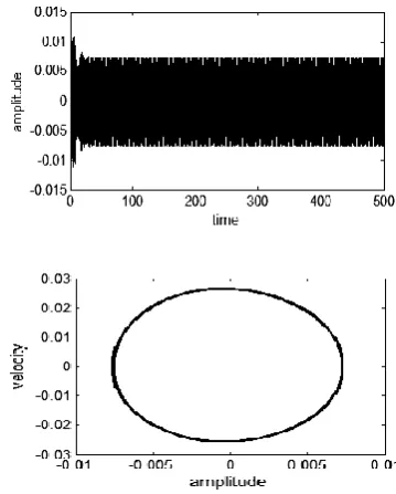
The Runge-Kutta fourth order method has been applied to determine the numerical solution of the given system at non-resonance case, as shown in Fig. 1, which is considered as basic case. We can see that the system is stable with steady state amplitude is about 0.007 and the phase plane is limit cycle.

A. Effects of parameters

From Fig. 2a, the amplitude is monotonic decreasing function in the damping coefficient



, and more increasing of the value of



leads to saturation phenomena. The amplitude is monotonic increasing in the natural frequency



and excitation frequencies



_j and the maximum amplitude occurs at primary resonance,

 

_j



, as shown if Figs. 2b, 2g respectively . Figs. (2c- 2f) show that the amplitude is monotonic increasing in the excitation

amplitudes

F

_j, but more increasing of

F

_j may leads to the system damage or uncontrolled.

B. Resonance cases

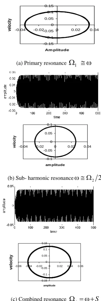
Some of the deduced resonance cases are confirmed numerically (Fig.3.). Table1 summarizes different considered cases. It can be seen that the simultaneous primary resonance case

 

_j



,

j



1, 2,3, 4

and

S



2 

is the worst case; the amplitude is about 700% of the basic case shown in Fig. 1

C. Frequency response curves

In this section, the stability zone and effects of the different parameters are discussed using frequency response equation (21). The steady state response of the given system at various parameters near the simultaneous resonance case is investigated and studied in Fig. 4. From this figure it can be seen that the steady state amplitude is monotonic decreasing function in the damping coefficient as shown in Fig. 4a. Also from Fig. 4b, the steady state amplitude is monotonic increasing function natural frequency



. The steady state amplitude is monotonic increasing function in the nonlinear parameters



₁ and the amplitudes of the excitation forces

j

F

as shown in Figs. 4c, 4e. But the steady state amplitude is monotonic decreasing function in the coefficient of the time varying stiffness



₂ as seen in Fig. 4d, this means that it can be use to control of the vibration of the system to be small .

(6)

Fig. 2. Effects of parameters

-0.15 -0.1 -0.05 0 0.05 0.1 0.15

-0.04 -0.02 0 0.02 0.04

Am plitude

ve

lo

ci

ty

1

  

(a) Primary resonance

-0.1 -0.05 0 0.05 0.1

-0.04 -0.02 0 0.02 0.04

am plitude

ve

lo

ci

ty

2

2   

(b) Sub- harmonic resonance

-0.15 -0.1 -0.05 0 0.05 0.1 0.15

-0.06 -0.04 -0.02 0 0.02 0.04 0.06

amplitude

v

e

lo

c

ity

j

S

(7)

-0.15 -0.1 -0.05 0 0.05 0.1 0.15

-0.04 -0.02 0 0.02 0.04

am plitude

ve

lo

ci

ty

2

j

S

  

(d) Combined resonance

-0.1 -0.05 0 0.05 0.1

-0.03 -0.02 -0.01 0 0.01 0.02 0.03

amplitude

v

e

lo

c

it

y

2

j

S

  

(e) Combined resonance

-0.1 -0.05 0 0.05 0.1

-0.04 -0.02 0 0.02 0.04

amplitude

v

e

lo

c

it

y

2

1 (

)

2 S

 

 

(f) Combined resonance

-0.15 -0.1 -0.05 0 0.05 0.1 0.15

-0.04 -0.02 0 0.02 0.04

amplitude

v

e

lo

c

ity

1

1 (2

₂

S

)

 

 

(j) Combined resonance

-0.15 -0.1 -0.05 0 0.05 0.1 0.15

-0.06 -0.04 -0.02 0 0.02 0.04 0.06

Amplitude

v

e

loc

it

y

resonance (h) simultaneous

1 2 3 4

,

S

2           

(8)

Fig. 4. Frequency response curves

Note that: Lc means Limit Cycle and MLC means Multi Limit cycle

IV. COCLUSIONS

A single degree of freedom of a cantilever skew of aluminum plate are introduced using quadratic and cubic non-linearities with time varying stiffness are considered and studied. The multiple time scale perturbation technique is applied. An approximate solution is derived up to third order approximation. The stability of the system investigated applying both frequency response functions and phase-plane methods. The effects of different parameters are studied numerically. From the above study the following may be concluded 1. The worst resonance case of the system is the

simultaneous resonance case and the system has a variety of interesting phenomenon such as multi-valued solutions, jump.

2. The steady state amplitude of the system is monotonic increasing function natural and excitation frequencies. 3. The amplitude is increasing function in the excitation

forces amplitudes.

4. The steady state amplitude is monotonic decreasing

2



, which can be use to control of the vibration of the system to be small if possible.

5. The system needs to vibration reduction or vibration control.

Table I

Summary of some investigated resonance cases

REFERENCES

[1] H. N. Arafat and A. H. Nayfeh," Non- Linear Responses of Suspended Cables Primary Resonance Excitation," Journal of sound and vibration, Vol. 266, No.22003, pp. 325-354. doi: 10.1016/S0022-460X (02)01393 [2] G. Zheng, J.M. Ko and Y. O. Ni, "Super-Harmonic and Internal

Resonances of a Suspended Cable with Nearly Commensurable Natural Frequencies, "on- Linear Dynamics, Vol. 30, No. 1, 2002, pp.55-70. doi: 10. 1023/A: 10203592293 92

[3] W. Zhang and Y. Tang, "Global Dynamics of the Cable under Combined Parametrical and External Excitations, "International Journal of Non-Linear Mechanics, Vol.37, No. 3, 2002, pp. 505-526. doi :10.1016/S002-7462(01)000269 [4] Y. A. Amer and M. Sayed, "Stability at a Principal Resonance

of Multi- Parametrically and Externally Excited Mechanical System ,"Advanced in Theoretical and Applied Mechanics,Vol. 4, No. 1, 2011, pp.1-14.

[5] M. Sayed, Y. S. Hamed and Y. A. Amer, "Vibration Reduction and Stability of Non-Linear System Subjected to External and Parametric Excitation Forces under a Nonlinear Absorber

Chaos Amplitude

ratio Case

Resonance type

LC 100%

No n- resonant

LC 506%

1

  

Primary

resonance

MLC 34%

1

2   

Sub-harmonic

resonance







2

356% LC

LC 342%

4

4 

 

M

L C

41%

1

2   

Super--harmonic resonance

LC 575%

1 2

s

   

 

Combined resonance

LC 506%

1 2

2 s

   

 

LC 383%

1

2 s

 

 

LC 370%

4 3

(

)

    

LC 32%

4 3

2     

(

)

LC 337%

2

1 (

)

2 s

 

 

LC 493%

1

1 (2

)

2 s

 

 

LC 465%

1

1 (2

)

2 s

(9)

[6] Cheng-Tang Lee et al., "Sub-Harmonic Vibration Absorber for Rotating Maclunery," ASME Journal of Vibration and Acoustics, 119(1997), 590-595.

[7] I. Y. Shen, W. Guc and Y. C. Pao, "Torsicnal Vibration Control of a Shaft through Active Constrained Layer Damping Treatments," Journal of Vibration and Acoustic 119(1997), 504-511.

[8] N. Liu and K. W. Wang, "A Non-dimensional Parametric study of Enhanced Active Constrained Layer Damping Treatments," Journal of Sound and Vibration, 223, No. 4(1999), 611-644. [9] R. Stanawy and D. Chantalkhana, "Active Constrained Layer

Damping of Clamped- Clamped Plate Vibration, "Journal of Sound and Vibration, 241, No. 5(2001), 755-777. [10] S. S. Oueini and A. H. Nayef, "Saturation Control of a DC

Motor," "AIAA-96-1642- Cp, 1996 [11] S. S. Oueini, A. H. Nayef and M. F. Golnaraghi," A

theoretical and Experimental Implementation of A Control Method Based on Saturation, "Non- Linear Dynamics, 13(1997), 189-202. Saturation, "Non- Linear Dynamics, 13(1997), 189-202.

[12] C. Park, C. Walz and I. Chopra, " Bending and Torsion Models of Beams with Induced Strain Actuators," The SPIE Smart Structures and Materials 93, Alburquerque, NM, 1993.

[13] B. Wen, A. S. Naser and M. J. Schulz, "Structural Vibration Control Using PZT Patches and

Non-Linear Phenomena, "Journal of Sound and Vibration215, No. 2(1998), 273-296.

[14] S. S. Oueini and A. H. Nayef," Single- Mode Control of a Cantilever Beamuder principal Parametric Excitation, "Journal of sound and Vibration, Vol. 224, No. 1, 1999, pp. 33-47. doi: 10.1006/jsvi.1998.2028

[15] K. R. Asfar," Effects of Non-Linearities in Electrometric Material Dampers on Torsional Vibration Control,"

International Journal of Non-LinearMechanics, Vol. 27, No. 6, 1992, pp. 947-954.

[16] M. Eissa and W. El-Ganaini," Part I, Multi- Absorbers for Vibration Control of Non-Linear Structures to Harmonic Excitations," Proceeding of ISMV Conference, Islamabad, 2000 [17] M. M. Kamel and Y. A. Amer," Response of Parametrically Excited One- Degree- of Freedom System with Non-Linear Damping and Stiffness," Physica Scripta, Vol. 66, No. 6, 2002, pp.410-416. doi: 10.1238/physica.Regular.066a 00410 [18] Y. A. Amer,"Vibration Control of Ultrasonic Cutting via

Dynamic Absorber," Chaos, Solutions and Fractals, Vol. 33, No.5, 2007, pp. 1703-1710. doi: 10.1016/j. chaos.2006.03.038 [19] M. Eissa and M. Sayed, "Vibration Reduction of a Three DOF

Non-Linear Spring Pendulum," Communication in Nonlinear Science and Numerical Simulation, Vol. 13, No. 2, 2008, pp.465-488. doi: 10.1016lj.cnsns.2006.04.00

[20] M. Sayed and Y. S. Hamed, "Stability and Response of a Non- Linear Coupled Pitch-Roll Ship Model under Parametric and Harmonic Excitations," NonlinearDynamics, Vol.