Boundary Element Model Updating Using Frequency
Response Functions
Nivaldo Benedito Ferreira Campos
1, José Maria Campos dos Santos
21Department of Structural Engineering, School of Civil Engineering, Architecture and Urbanism, UNICAMP
2Department of Computational Mechanics, College of Mechanical Engineering, UNICAMP.
1
[email protected], [email protected]
Abstract – In order to model the dynamic behavior of complex structures it is required numerical models with high accuracy. These models generally are obtained by using numerical methods such as finite element method, finite difference method, and boundary element method, the latter having become an interesting option compared to the other two. Nevertheless, rarely the dynamic behavior of a real structure will match that obtained with its numerical model. To overcome this problem, an alternative it to use model updating techniques. In this work, it is presented a technique of model updating based in correlating an experimental frequency response function (FRF) with one from a boundary element method model. The correlation is evaluated through an objective function consisting in the sum of the squared differences between the FRFs. Several cases were considered to present the boundary element method model updating technique. The results obtained usind boundary element model were compared with those from the updating of finite element models.
Index Term -- model updating, boundary element method, beams, frequency response function
1. INTRODUCTION
The importance of structural model updating methods in the dynamic structural analyses is well recognized. A class of these techniques consists in minimizing the differences between the numerical model related to measurements data taken during a physical test, by using a parameter estimation procedure [1-3]. In structural dynamic testing it is common practice to measure the data in the form of frequency response functions (FRF). From de measured FRFs an experimental model of the structure dynamic behavior can be obtained. To use FRFs data is more generally applicable because it is not always possible to extract from them a good modal model, specially when the measured data set are incomplete or the system has high modal density.
The knowledge about a particular structure is contained in a theoretical model, which can be constructed using a numerical method. A large number of papers written with on the subject have used the finite element method (MEF) as the base for numerical model [4]. However, in recent years boundary element method (BEM) has been successfully applied to numerical solution of many engineering problems, and for some classes of problems has been proven to be competitive with the FEM [5].
Our purpose in this work is to develop an algorithm to solve the model update problem of flexural beam vibration
based on the BEM in its direct form [6]. The parameter estimation algorithm is made via the curve fit of measured FRFs using a non-linear least-squares method [7]. Although the problem does not seems to pose a great difficulty, it has not been previously treated in a model updating sense. The method is simulated with the Friswell & Mottershead’s beam example [3], where the estimated parameters are the same (beam’s flexural rigidity, translational and rotational spring stiffness of a flexible joint) but the experimental data are the FRFs instead modal parameters. Numerical simulation results using a pseudo-experimental data are shown and compared with a similar finite element model updating method.
2. DYNAMIC BOUNDARY ELEMENT FORMULATION FOR
BEAMS
This section presents a brief theoretical review of BEM formulation for axial and flexural vibration in beams [6]. The differential equations governing the time domain dynamic axial and flexural behavior of a rectilinear beam, with constant geometric and material properties along x-axis, are given, respectively, by:
2 2
2 , 2
u u u
AE c p x t A t
x t
(1)
4 2
4 2 ,
v v v EI A c q x t
t x t
(2)
where I and v represent the axial and flexural displacements,
A is the cross section area, EI is the beam flexural rigidity, p and q are the distributed axial and transversal loads, c is the
coefficient of viscous damping and is the material density.
Assuming stationary dynamic behavior, the displacements and excitations in equations (1,2) may be generically written as
a(x,t) = a(x)exp(it), where is the circular frequency. Under
this assumption, equations (1) and (2) take, respectively, the form
22
2 u
p x d u
u λ
AE
dx , where
2 2
u
ρω i c λ
E
(3)
44
4 v
q x d v
v λ
EI
dx , where
2 4
v
ρAω i c λ
EI
(4)
fundamental solution. For equation (1) the fundamental solution is given by [6]:
1
2 2sin
2 u u
u x, y λr a b AE
λ
(5)
where x is the observation point, y is the source point and r x
- y. For equation (2) the fundamental solution is:
3
1
sec sin sech sinh
4 v v v v v
v x, y λ L λ L ξ λ L λ L ξ EI
λ
(6)
where x y.
The differential equations and the fundamental solutions given above can be applied to a standard BEM formulation to yield the uncoupled Boundary Integral
Equations (BIE) governing, respectively, the axial (u) and the
flexural (v) displacements and the rotation () response of a
rectilinear beam of length L, resulting in
0 0 0 L L Lu y u x N x, y N x u x, y
p x u x, y dx
(7)
0 0 0
0 0
L L
L
L L
v y V x v x, y M x θ x, y θ x M x, y
v x V x, y q x v x, y dx
(8)
0 0 0 0 0 L L L L Ldv x, y dθ x, y
θ y V x M x
dy dy
dV x, y dv x, y
θ x v x q x dx
dy dy
(9)
where the functions N, , M and V are given by:
du N AE dx ; dx v d
θ ; 2 2
dx v d EI
M ; 3 3
dx v d EI
V (10)
Applying the collocation point y at the boundaries of
the element (y 0 and y L), and performing the domain
integrals of the distributed loads, two algebraic systems of
equations may be written for the axial and flexural behavior of the element. Equations (11) and (12) show the resulting systems of equations, for the case of one internal point
situated at y1:
1 1 1 1 1 1
0 0 1 0 0 0 0 0 0 0
0
0 1 0 0
0 1 0
N , N L, u u , u L, F N
N ,L N L,L u L u ,L u L,L F L N L N ,y N L,y u y u ,y u L,y F y
(11)
11 1 1 1
1
0
0 0 1 0 0 0 0 0
0
0 0 0 0 1 0 0 0
0 0 1 0
0 0 1 0
0 0 1
0 0 0 0 0 0 0 0 0 0 0 0 v V , M , V L, M L,
θ V , M' , V' L, M' L,
v L V ,L M ,L V L,L M L,L
θ L V' ,L M' ,L V' L,L M L,L
v y V , y M , y V L, y M L, y
θ , v , θ' , v' , θ v ,L v' ,L v , y
1 1 1 1 0 0 0 0 0 0 0 0 0 0 θ L,v L, Q V θ' L,
v' L, Q' M
,L v L,L θ L,L Q L V L v' L,L
θ' ,L θ' L,L Q' L M L
Q y v L, y
θ ,y θ L,y
(12)
where
0
L
F y
p x u x, y dx,
0L
Q y
q x v x, y dxand the primes in equation (12) indicate differentiation with
respect to y.
Provided the proper boundary conditions are considered, equations (11) and (12) describe completely the uncoupled axial and flexural dynamic response of one rectilinear structural element within the frequency domain. Equation (11) and (12) can be rewriting in a more compact form as
a a a a
au Bn f
A (13)
f f f f
fu Bn f
A
(14)
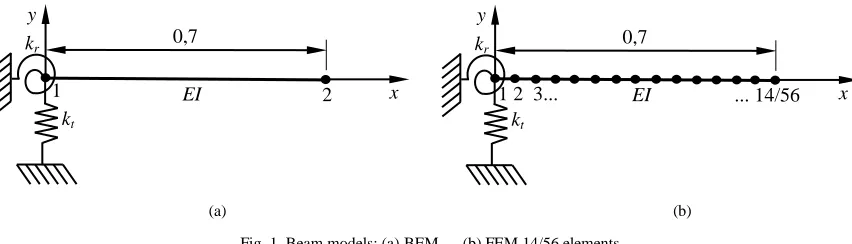
Now the boundary conditions must be applied to the specific structure. The Friswell & Mottershead’s beam example consists of an aluminum cantilever beam with
bending only in vertical plane (Figure 1). .
(a) (b)
Fig. 1. Beam models: (a)BEM (b) FEM 14/56 elements.
0,7 kr EI y x kt 1 2 0,7 kr EI y x kt
The clamped side is replaced by a flexible joint with a translational and rotational spring stiffness, generating the boundary conditions
0 t (0);
0 r
0 ;
0; ( ) 0V k v M -k V L M L (15)
where kt and kr are translational and rotational spring stiffness
coefficient, respectively. By applying equations (15) into equation (12) and rearranging we obtain
1 1 1 1
1 1
0 0 1 0 0 0 0 0 0 0 0 0 0 0 0 1 0 0
0 0 0 0
0 0 0 0
0 0 0 0
0 0 0
0 0 0
1 0 1 0 1 t r t r t r t r t r
V , k v , M , k θ , V' , k v' , M' , k θ' , V ,L k v ,L M ,L k θ ,L V' ,L k v' ,L M' ,L k θ' ,L V , y k v , y M , y k θ ,y
V L, M L, V' L, M' L, V L,L M L,L
V' L,L M L,L V L, y M L, y
1 1 0 0 0 0 v Q θ Q' v L Q L θ L Q' L v y Q y (16)
Equation (16) in a more compact form is
f f f
G w q (17)
By applying a unit force in the point x1 and solving the
equations (17) for wf , we obtain the receptance FRFs for the
flexural dynamic response v(y1).
3. NONLINEAR LEAST-SQUARES
This section presents a brief theoretical review of nonlinear least-squares formulation [7]. Mathematically the inverse sensitivity method corresponds to nonlinear least
squares problem. Given the sensitivities, S, of some dynamic
function such as analytical FRFs, HA, with respect to a set of
analytical model parameters, p,
A H S p (18)
it is possible to obtain a correction of the parameter values
from the difference between HA and corresponding
experimental values HX. As the analytical FRF is nonlinear in
respect to the parameters this is an iterative procedure with all the possible associated convergence problems, and there is necessary to evaluate the analytical function at each iteration.
The corrected parameters at iteration k+1 are given by
1
k k
p p p (19)
where:
XX AA
S H H
p
S H H
(20)
and is the step size, a scalar parameter used to improve the
convergence process. To determine the step size was
introduced an algorithm that use a cubic interpolation line
search in the direction of p, to obtain the minimization of the
total squared error function, given by:
H
X A X A
ε p H H H H (21)
To start the iterative procedure, initial analytical parameters are guessed. The sensitivity matrix is calculated using finite difference approach. In order to avoid high computational cost of nonlinear search the first difference was used, which can be written as:
i i
i A j j A j
A ij
j j
H p p H p
H S p p
(22)
The sensitivity precision is highly influenced for the p
choice. In that case was used the same criteria as [7]. Also, the method can be further enhanced into a Bayesian estimation [1] if there is some knowledge about the statistics of the errors present in the experimental data and the analytical model parameters.
4. SIMULATION EXAMPLE
Performance of the boundary element model updating algorithm was verified by analyzing the Friswell & Mottershead’s beam example. The beam has 0.7m length, 50mm x 25mm cross section and only bending in vertical plane is considered. The estimated parameters are the beam’s
flexural rigidity (EI), translational (kt) and rotational (kr)
spring stiffness of the flexible joint. For ease of comparison, some modifications were made in the original example. The experimental data are the FRFs instead modal parameters. Viscous damping was introduced in the BEM (damping coefficient) and FEM (mass and stiffness proportional damping) models to obtain good correspondence between analytical and experimental models. Two values of damping
coefficient were used, c= 50 N.s/m and c= 100 N.s/m, while
for the mass and stiffness proportionality coefficients the
values, = 29.851 and = 1.5113E-12, were used
respectively, which reproduce a damping equivalent to
c = 100 N.s/m. Since BEM model contains a simple element
and his formulation is analytically exact, the pseudo-experimental FRFs data were obtained from this model with 6000 lines in the frequency range of 0.5-3000 Hz.
To simulate the realistic case of noisy measurements, the pseudo-experimental FRF’s were corrupted with a random noise of the form
1,1
100ij ij ij
f
H H H rand (23)
where Hij is the FRF measured at station i for an excitation
force at station j, f is the noise scale factor, rand[-1,1] is a
random number uniformly distributed between -1 and 1, Hij
is the noise-polluted FRF.
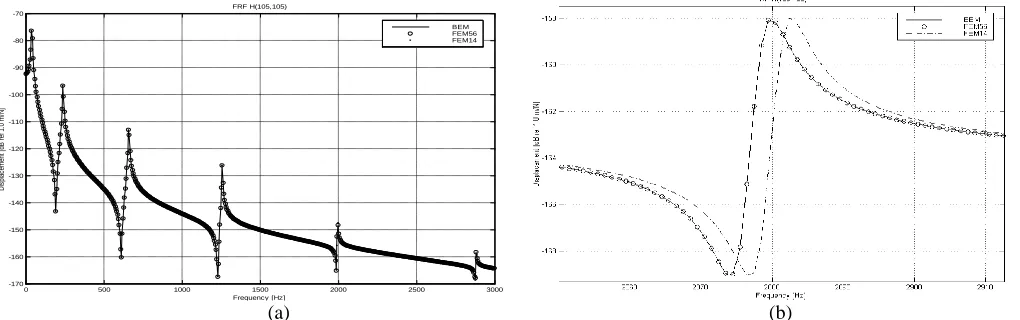
Figure 2a shows a comparison between FRFs H105,105 obtained by FEM models with 14 and 56 elements, and BEM model with one element. Apparently the tree curves agree, however, if a zoom is made in the last peak of this FRFs (Figure 2b), it can be seen that only those generated by BEM and FEM with 56 elements agree. The disagreement of the FRF generated by FEM with 14 elements come from the approximations of FEM formulation.
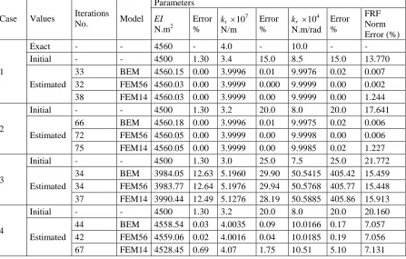
A first evaluation of the BEM model update precision and convergence was made in a frequency range of
0.5-1000 Hz. As in reference [5], 1.3% error to EI and 50%
error to kt and kr were used. Table 1 shows the exact, initial
and estimated parameters values from BEM and MEF with 14/56 elements model updating with damping coefficients
c = 100 N.s/m, and using pseudo-experimental FRFs with
noise levels of 1%, 5%, 10% and 20%. It can be seen that in
all the cases estimated parameters converge to or are very close (less than 5% error) to the correct solution. The errors in the estimation grow higher as the noise levels increase. Similar behavior can be observed with the FRFs norm error. Only the number of iteration presents a significant difference, with BEM models taking less iterations then FEM14 and FEM56. This does not necessarily means an advantage since the FEM14 needs less computation time then the others for the given number of iterations. Although not shown in the paper, results for BEM model updating using c = 50 N.s/m presented a similar behavior as the case for c = 100 N.s/m. Figure 3 shows a comparison of the FRFs obtained for BEM model with 20% of noise level determined by tree distinct procedures: the pseudo-experimental, the one calculated from initial parameters and using the update model. The same behavior was found in FEM model updates.
(a) (b)
Fig. 2. FRFs H105,105 obtained by BEM, MEF 56 elements and MEF 14 elements: (a) total frequency range; (b) zoom in the last peak
Another evaluation was made considering a wider range from 0.5 Hz to 3000 Hz. The error percentage of the initial parameters was kept the same of the previous
evaluation, 1.3% for EI and 50% for the spring coefficients (kt
, kr). It has been observed that this error percentage on the
initial spring coefficients will increases the differences in the higher frequency peaks of the initial and experimental FRFs. Under this circumstances the update process converges to incorrect parameter values. This is a common behavior of
FRFs based model update procedures and has its origin in the existence of local minima which leads to wrong solutions, far from the global minimum. In order to evaluate this effect tree cases with spring coefficient errors of 15, 20 and 25% without FRF noise were analyzed. A fourth case was verified using 20% of error on spring coefficients and 20% FRF noise. Table 2 shows the estimated parameters values from BEM and FEM 14/56 elements model updating.
Fig. 3. FRFs H105,105 pseudo-experimental with 20% noise level (Experimental), calculated with initial parameters (Initial) and updated (Updated) with BEM.
0 500 1000 1500 2000 2500 3000 -170
-160 -150 -140 -130 -120 -110 -100 -90 -80 -70
FRF H(105,105)
Frequency [Hz]
D
is
pl
ac
em
en
t
[d
B
r
ef
1
.0
m
/N
]
BEM FEM56 FEM14
0 100 200 300 400 500 600 700 800 900 1000 -170
-160 -150 -140 -130 -120 -110 -100 -90 -80 -70
FRF H(105,105)
Frequency [Hz]
D
is
p
la
c
e
m
e
n
t
[d
B
r
e
f
1
.0
m
/N
]
Experimental Updated Initial
Table I
Exact, initial and estimated parameters values from BEM, MEF 14 elements, and MEF 56 elements model updating with c = 100 N.s/m ( = 29.851, = 1.5113E-12) and f = 0,1, 5, 10 and 20 %.
Values Iterations
Number FRF Noise (%)
Parameters
FRF Norm Error (%) EI
N.m2
Error %
kt 107
N/m
Error %
kr 104
N.m/rad Error
% Initial Estimated
Exact
- - 4560 - 4.0 - 10.0 - - -
Initial 4500 1.30 2.0 50.0 5.0 50.0 - -
BEM Estimation
37 0 4559.99 0.000 4.0000 0.000 10.0000 0.000 46.646 0.000
35 1 4559.13 0.019 4.0073 0.182 10.0032 0.032 46.685 0.331
36 5 4562.81 0.062 3.9808 0.480 9.9799 0.201 46.399 1.739
34 10 4573.62 0.299 3.9388 1.530 9.8568 1.432 47.651 4.193
36 20 4618.87 1.291 3.6785 8.038 9.5165 4.835 48.806 7.135
FEM14 Estimation
70 0 4559.86 0.003 3.9941 0.148 10.0035 0.035 46.646 0.013
55 1 4558.86 0.025 4.0015 0.038 10.0070 0.070 46.685 0.332
51 5 4562.67 0.059 3.9750 0.625 9.9834 0.166 46.398 1.742
50 10 4573.50 0.296 3.9330 1.675 9.8599 1.401 47.651 4.187
59 20 4617.99 1.272 3.6779 8.052 9.5239 4.761 48.806 7.134
FEM56 Estimated
70 0 4560.00 0.000 4.0000 0.000 10.0000 0.000 46.646 0.000
54 1 4559.13 0.019 4.0073 0.182 10.0032 0.032 46.685 0.331
51 5 4562.81 0.062 3.9808 0.480 9.9800 0.200 46.398 1.739
50 10 4573.62 0.299 3.9388 1.530 9.8568 1.432 47.651 4.193
61 20 4617.89 1.270 3.6823 7.943 9.5266 4.734 48.806 7.133
Table II
Estimated parameters results from BEM, MEF 56 and 14 elements model updating algorithm to Case 1, 2 and 3 with 15, 20 and 25 % error in kt and kr , without
FRF noise; and Case 4 with 20% error in in kt and kr , with 20% FRF noise.
Case Values Iterations
No. Model
Parameters
EI
N.m2
Error %
kt 10
7
N/m
Error %
kr 10
4
N.m/rad
Error %
FRF Norm Error (%)
1
Exact - - 4560 - 4.0 - 10.0 - -
Initial - - 4500 1.30 3.4 15.0 8.5 15.0 13.770
Estimated
33 BEM 4560.15 0.00 3.9996 0.01 9.9976 0.02 0.007
32 FEM56 4560.03 0.00 3.9999 0.000 9.9999 0.00 0.002
38 FEM14 4560.03 0.00 3.9999 0.00 9.9999 0.00 1.244
2
Initial - - 4500 1.30 3.2 20.0 8.0 20.0 17.641
Estimated
66 BEM 4560.18 0.00 3.9996 0.01 9.9975 0.02 0.006
72 FEM56 4560.05 0.00 3.9999 0.00 9.9998 0.00 0.006
75 FEM14 4560.05 0.00 3.9999 0.00 9.9985 0.02 1.227
3
Initial - - 4500 1.30 3.0 25.0 7.5 25.0 21.772
Estimated
34 BEM 3984.05 12.63 5.1960 29.90 50.5415 405.42 15.459
34 FEM56 3983.77 12.64 5.1976 29.94 50.5768 405.77 15.448
37 FEM14 3990.44 12.49 5.1276 28.19 50.5885 405.86 15.913
4
Initial - - 4500 1.30 3.2 20.0 8.0 20.0 20.160
Estimated
44 BEM 4558.54 0.03 4.0035 0.09 10.0166 0.17 7.057
42 FEM56 4559.06 0.02 4.0016 0.04 10.0185 0.19 7.056
67 FEM14 4528.45 0.69 4.07 1.75 10.51 5.10 7.131
.
the spring coefficients above which the parameter estimation algorithm will converge to the wrong solution. Case 4 can be seen as an indicator that if the initial FRF is in the solution space of the global minimum a noisy experimental FRF (20% noise) will not deviate the method from converging to the correct values.
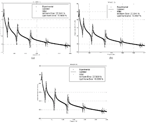
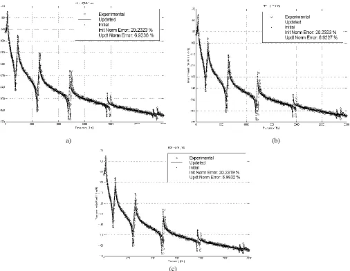
Figures 4-5 shown the FRFs H105,105 from BEM and FEM models calculated with initial parameter, updated and pseudo-experimental values in the frequency range of 0.5-3000Hz for the case 3 (Figure 4) and case 4 (Figure 5). Except for the case 3 the updated model reproduced the experimental FRF in all frequency range with a very low norm error.
(a) (b)
(c)
a) (b)
(c)
Fig. 5. FRFs H105,105 Initial with spring coefficient errors of 20%, pseudo-Experimental with 20% noise and Updated: (a) BEM (b)FEM56 (c)FEM14.
5. FINAL REMARKS
A scheme for structural boundary element model updating using frequency response functions as measurement data was presented. The proposed procedure was verified with simulated BEM model example and compared with the results of FEM model. The boundary element formulation of axial and flexural structural dynamics in beams and nonlinear least-square parameter estimation were briefly reviewed. The proposed method was verified for different error in the unknown parameters, in the presence of simulated noisy pseudo-experimental FRF. In a general sense, the results show that the behavior of BEM model update is similar to the FEM model update, and some of the hard problems still are in the parameter estimation procedures. That fact is an indication that the choice as to use one method or another must be decided by taking in account the strength and the weakness in the application of each method. However, it must be admitted that this study represents a simulation test of the procedure. To perform a better evaluation of the BEM model update strategy, two other aspects must be considered in future work. The first
is to use real measured experimental data. The order issue is the dimensionality of the problem. In this paper a 1-D problem was treated and it is recognized that 2D and 3D BE models tend to be more efficient than their FEM counterpart.
REFERENCES
[1] Natke, H. G., Updating of computational models in the frequency domain based on measured data: A survey, Probabilistic Engineers Mechanics, 3, 28-35, 1988.
[2] Beck, J. V. and Arnold, K. J., Parameter estimation in engineering and science, New York, John Wiley, 1977.
[3] Friswell, M. I. and Mottershead, J. E., Finite element model updating in structural dynamics, London, Kluwer, 1995.
[4] Mottershead, J. E. & Friswell, M. I., Model updating in structural dynamics: a survey, Journal of Sound and Vibration, 167(2), pp. 347-373,1993.
[5] Banerjee, P. K. and Butterfield, R., Boundary element methods in engineering science, London, McGraw-Hill, 1981.
[6] Mesquita Neto, E., Barretto, S. F. A. and Pavanello, R., Dynamic behavior of frame structures by boundary integral procedures. Engineering Analysis with Boundary Elements (submitted).