Parallelization of 3-D ADI Scheme on Telegraph Problem
using Domain Decomposition with PVM
Ewedafe Simon Uzezi
Faculty of Computing and IT Baze University Abuja, Nigeria
Rio Hirowati Shariffudin
Institute of Mathematical Sciences Faculty of Science
University of Malaya
ABSTRACT
A parallel implementation of 3-D Alternating Direction Implicit (3-D ADI) method on 3-D Telegraph problem on a distributed computing environment through Parallel Virtual Machine (PVM) is reported. The numerical method is implicit and is based on a splitting strategy which is applied alternately at each half time step. The parallelization is implemented by a Domain Decomposition (DD) strategy on a distributed system with Single Program Multiple Data (SPMD) model on a PVM platform. The parallelization strategy and performance are discussed. Different strategies to improve the computational efficiency are proposed.
General Terms
Parallel Computing, Numerical Computing, Mathematical Computation.
Keywords
Telegraph, 3-D ADI, PVM, Domain Decomposition, and Parallelization.
1.
INTRODUCTION
Due to the ever-increasing clock frequency and the aggressively shrinking feature sizes of the very large scale integration technology, robust power distribution network is crucial to ensure the quality of power delivery. This makes the issues of parallel and distributed applications very important. Parallel computing environments based on distributed computing has become effective and economical platforms for high performance computing by providing controlled access to a much larger and richer computational resource [20]. Distributed systems can increase application performance by significant amount and the incremental enhancement of a network based concurrent computing environment is usually straight forward because of the availability of high bandwidth networks [2, 3]. Attempts have also been made towards parallel solutions on distributed memory MIMD machines. Large scale computational scientific and engineering problem, such as time dependent and 3D flows of viscous elastic fluids, required large computational resources with a performance approaching some tens of giga (109) floating point calculations per second, an alternative and cost effective means of achieving a comparable performance is by way of distributed computing, using a system of processors loosely connected through a local area network [4]. Relevant data
need to be passed from processor to processor through a message passing mechanism [12, 6, 19, 16]. The natural programming style under a distributed system is therefore the Multiple Instructions Multiple Data (MIMD) [22]. The basic idea is to split a program into a few smaller tasks and to allocate these tasks to several processors to be executed simultaneously. Thus the total execution time can be reduced to just a fraction of that of a uni-processor computer. Generally, there are three issues relating to parallel computing: (1) The first issue is how to break up the program into smaller tasks, and how to properly sequence these tasks, (2) The second is the communication between processors, which is necessary because some intermediate results have been exchanged among these processors and (3) The issue of the synchronization of computations on different processors. All these three problems strongly influence the performance of the parallel computation.
Methods by which processors exchange information; parallel computers can either be of shared memory or distributed memory (message-passing) architectures. With the shared memory architectures, there is a global share memory which can be accessed by all processors. Processors communicate by writing into and reading from the global memory. This mode of communication is convenient in terms of program writing, but memory access by different processors can generate potential memory conflicts. With distributed memory architectures, each processor has its local memory, and processors communicate through an interconnection network. Inefficient communication is the main problem for this type of communication. To help with the program development under a distributed computing environment, a number of software tools have been developed: PVM, Theoretical Chemistry Message Passing Tool Kit (TCMSG), Parasoft Express (EXPRESS), Network Linda (LINDA), and Message Passing Interface (MPI). PVM [13, 14] is chosen here since it has a large user group with possibly the best support for heterogeneous environment.
functional decompositions have also been used in parallel implementations.
In this paper, we present a parallel program for the solution of the 3-D Telegraphic problem using the 3-D ADI method. We employed the DD strategy, and mapped it onto a distributed computing environment with a synchronous iteration and a message passing master – slave construction. The program was executed in a distributed memory system under PVM. The numerical method is based on the double sweep methods of Peaceman and Rachford (DS-PR) [19]. We computed some examples to test the parallel algorithm. The effects of the various parameters on the performance of the algorithm are discussed. The prime objective of our platform is not to be specific to one problem; it should be able to solve a wide variety of time-dependent partial differential equations (PDE) for various applications [24, 25]. This paper is organized as follows: Section 2 introduces the model for the 3-D Telegraphic problem and introduces the 3-D ADI method. Section 3 introduces the parallel implementation. Section 4 introduces the results and discussion. Finally, a conclusion is included in section 5.
1.1
Previous Research Work
The ADI method for the partial differential equations (PDEs) proposed by Peaceman and Rachford [16] has been widely used for solving algebraic systems resulting from finite difference method analysis of PDEs in several scientific and engineering applications. On the parallel computing front, Rathish Kumar, et. al., have proposed a parallel ADI solver for linear array of processors. Chan and Saied have implemented ADI scheme on hypercube. Later Lixing et. al., have parallelized the ADI solver on multiprocessors. The ADI method in [18] has been used for solving heat equation in 2-D. Other works on parallel implementation of 2-D Telegraph problem on cluster systems have been done in [10, 11]. Hence, parallelization of the ADI method has been tried in [22]. Several numerical approaches dealing with telegraphic equation problems have been carried out in [1, 8] and [9]. In [15] the unconditional stability of the alternating difference schemes has similarity to our scheme and shows that the unconditional stability application is useful to its speedup and efficiency as studied. Our implementation compared to others is a way of proofing stability and convergence in parallel platform of a distributed system. We also note the various constant improvement on speedup, efficiency performance analysis in [25] using the overlapping domain decomposition method.
2.
TELEGRAPH EQUATION
the frequency and time domains. A number of iterative methods are developed in the literature to solve the Telegraph equation using iterative solution [18]. Some of these iterative schemes are employed in various parallel platforms [2, 20]. The speed of convergence of iterative scheme is examined for the synchronous communication approaches in parallel environment. We consider the second order Telegraph
equation:
0
2 2 2 2 2 2 2 2
z
v
y
v
x
v
t
v
a
t
v
(2.1)where
a
RC GL
, let
x
,
y
and
z
be the grid spacing in the x, y, z and t directions, wherem
z
y
x
1
/
, m is a positive integer. Hence, we can solve (2.1) by extending the 1-D simple implicit finite difference method [8] of the Telegraph equation to the above 3-D Telegraph equation, (2.1) becomes:0
)
(
2
)
(
2
)
(
2
2
)
(
2
2 1 1 , , 1 , , 1 1 , , 2 1 , 1 , 1 , , 1 , 1 , 2 1 , , 1 1 , , 1 , , 1 1 , , 1 , , 2 1 , , , , 1 , ,
z
v
v
v
y
v
v
v
x
v
v
v
t
v
v
a
t
v
v
v
n k j i n k j i n k j i n k j i n k j i n k j i n k j i n k j i n k j i n k j i n k j i n k j i n k j i n k j i (2.2)although this simple implicit scheme is unconditionally stable, we need to solve a heptadiagonal system of algebraic equations at each time step. Therefore, the computational time is extremely huge.
2.1
3-D ADI Method on the Telegraph
Problem
In this section, we derive the 3-D ADI method of the simple implicit finite difference method by using a general ADI procedure [18] extended to (2.1). The ADI method is a well-known method for solving the partial differential equation (PDE). The main feature of ADI is to sweep directions alternatively. In contrast to the standard finite-difference formulation with only one iteration to advance from the nth to (n + 1)th time step, the formulation of the ADI method requires multilevel intermediate steps to advance from the nth
to (n + 1)th time step. Equation (2.2) can be rewritten as:
0
2
1 , , 1 , , 1 , , 3 1
n k j i n k j i o n k j i mm
v
C
v
C
v
A
I
(2.3)where the operators of I, Ams, and the constants of Co, C1are
define as:
n
k j i n k j i n k j i x n k ji
v
v
v
v
A
1 , ,
1, ,
2
, ,
1, , (2.5)
n
k j i n k j i n k j i y n k j
i
v
v
v
v
A
2 , ,
, 1,
2
, ,
,1, (2.6)
n
k j i n k j i n k j i z n k j
i
v
v
v
v
A
3 , ,
, , 1
2
, ,
, , 1 (2.7)
t
a
t
t
C
o2
)
(
1
)
(
1
22 (2.8)
t
a
t
t
a
t
C
2
)
(
1
2
)
(
1
2 21 (2.9)
the constant of
x,
yand
zare:
t
a
t
x
b
x2
)
(
1
)
(
2 2
(2.10)
t
a
t
y
b
y2
)
(
1
)
(
2 2
(2.11)
t
a
t
y
b
y2
)
(
1
)
(
2 2
(2.12)Table 1. The 3-D ADI Algorithm
The 3-D ADI Algorithm
Input =
v
in,j,k,
v
in,j1,k
i
,
j
,
k
Output =
v
in,j1,k
i
,
j
,
k
Begin Sub-Iteration 1:
k
j
i
v
C
v
C
v
A
A
v
v
v
n k j i n k j i o n k j i n j i x n k j i x n k j i x,
,
)
2
(
)
(
)
2
1
(
1 , , 1 , , (*) 1 , , 3 2 ) 1 ( 1 , 1 ) 1 ( 1 , , ) 1 ( 1 , , 1
Sub-Iteration 2:k
j
i
v
A
v
v
v
v
n k j i n k j i n k j i y n k j i y n k j i y,
,
.
)
2
1
(
(*) 1 , , 2 ) 1 ( 1 , , ) 2 ( 1 , 1 , ) 2 ( 1 , , ) 2 ( 1 , 1 ,
Sub-Iteration 3:k
j
i
v
A
v
v
v
v
n k j i n k j i n k j i z n k j i z n k j i z,
,
.
)
2
1
(
(*) 1 , , 3 ) 2 ( 1 , , ) 3 ( 1 1 , , ) 3 ( 1 , , ) 3 ( 1 1 , ,
End and set 1 , , , , (*) 1 , ,2
nk j i n k j i n k j
i
v
v
v
(2.13)which is a prediction of
v
in,j1,kby the extrapolation method. Then splitting (2.3) by using an ADI procedure as in [18], we get a set of recursion relations as follows:)
2
(
)
(
)
(
1 , , 1 , , 0 (*) 1 , , 3 2 ) 1 ( 1 , , 1
n k j i n k j i n k j i n k j iv
C
v
C
v
A
A
v
A
I
(2.14) (*) 1 , , 2 ) 1 ( 1 , , ) 2 ( 1 , , 2)
(
I
A
v
injk
v
injk
A
v
injk (2.15) (*) 1 , , 3 ) 2 ( 1 , , ) 3 ( 1 , , 3)
(
I
A
v
injk
v
injk
A
v
injk (2.16)where
v
in,j1,k(1),
v
in,j,1k(2) are the intermediate solutions and the desired solution isv
in,j1,k
v
in,j,1k(3). Finally, expanding A1, A2and A3 on the left side of (2.14) and (2.16), we get the 3-D
ADI algorithm as in Table 1.
3.
PARALLEL IMPLEMENTATION
3.1
The Parallel Platform
3.2 Domain Decomposition
The parallelization of the computations is implemented by means of grid partitioning technique [5]. The computing domain is decomposed into many blocks with reasonable geometries. Along the block interfaces, auxiliary control volumes containing the corresponding boundary values of the neighboring block are introduced, so that the grids of neighboring blocks are overlapped at the boundary. When the domain is split, each block is given an I-D number by a “master” task, which assigns these sub-domains to “slave” tasks running in individual processors. In order to couple the sub-domains’ calculations, the boundary data of neighboring blocks have to be interchanged after each iteration. The calculations in the domains use the old values at the sub-domains’ boundaries as boundary conditions. This may affect the convergence rate; however, because the algorithm is implicit, the blocks strategy can preserve nearly same accuracy as the sequential program.
3.3
Parallel Algorithm
The algorithm can be transformed to master-slave model by sending out the computing tasks on each block to each processor in the Armadillo Generation Cluster system. The master task reads in the input data file, generates the grid data, initializes the variables, and sends all the data and parameters to the slaves. It then sends a block 3-D to each slave process, which in turn computes the coefficients of the relevant equations and solves for the solution of this block. This solution is then sent back to the master task and this processor wait for the next task. The master task receives the solution results from the slaves sequentially in an asynchronous manner, rearranges the data, calculates the global residuals of each equation, and determines if convergence has been reached. If the convergence has not been reached, the current solution vector is sent to all slaves, and a new iteration is started. Therefore, all the variables stored in the local memory of slaves are updated at every iteration. The following pseudo codes summarize the algorithm for the master and the slave program:
Master Program
Read in the input data
Compute mesh data
Initialize the variables
Enroll master program in pvm
Startup a slave program on each processor in the pvm farm
Send mesh data to all slave programs
Loop over iteration
Set block numbers and it value
Set the block index to it (ip = it)
Do while (slaves working on ip < n blocks)
if (ip < nblocks) then
do (for each processor)
if (processor is idle) then
ip = ip + 1
Send a
message to the idle processor to
Compute a solution on block ip
end if
if (ip = nblocks) break
end do
end if
wait here for a result from slave program
get block solution and residual of equation
end do while
Global residual calculation
Convergence check
if (solution converged) break out loop
send the current solution to all slave programs
end loop
Terminate all slave programs
Leave pvm
Time calculation
Save data file
Terminate the program
Slave Program
Enroll slave program in pvm
Do (forever)
Case:
GET MESH DATA
Get mesh data from the master program
Break
DO DOMAIN DECOMPOSITION
Break
GET CURRENT SOLUTION
Get the current solution vector
Break
DO CALCULATION
Get the block id, ip
Do calculation on block ip
Solve for all variables equation on block ip
Return the solution over ip to the master program
Break
FINISH UP
Leave pvm
Terminate the program
End case
End do
3.4
Speedup and Efficiency
The performance metric most commonly used is the speedup and efficiency which gives a measure of the improvement of performance experienced by an application when executed on a parallel system [21]. Speedup is the ratio of the serial time to the parallel version run on N processors. Efficiency is the ability to judge how effective the parallel algorithm is expressed as the ratio of the speedup to N processors.The concept of speedup has yet to find a widely accepted definition. In traditional parallel systems it is widely define as:
n
n
S
n
E
n
T
s
T
n
S
,
(
)
(
)
)
(
)
(
)
(
(3.1)where S(n) is the speedup factor for the parallel computation,
T(s) is the CPU time for the best serial algorithm, T(n) is the CPU time for the parallel algorithm using N processors, E(n)
is the total efficiency for the parallel algorithm. However, this simple definition has been focus on constant improvements. A generalized speedup formula is the ratio of parallel to sequential execution speed. A thorough study of speedup models, together with their advantages and disadvantages, is presented by Sahni [23], and observed that speedup is normally defined as the execution time of the best sequential algorithm also known as absolute speedup, therefore implying that the sequential and parallel might be different. A different approach known as relative speedup, considers the parallel and sequential algorithm to be the same. While the absolute speedup calculates the performance gain for a particular problem using any algorithm, relative speedup focuses on the performance gain for a specific algorithm that solves the problem. The total efficiency is usually decomposed into the following equations
),
(
)
(
)
(
)
(
n
E
n
E
n
E
n
E
num par load (3.2)where Enum, is the numerical efficiency, represents the loss of
efficiency relative to the serial computation due to the variation of the convergence rate of the parallel computation.
Eloadis the load balancing efficiency, which takes into account
the extent of the utilization of the processors, and Eparis the
parallel efficiency, which is define as the ratio of CPU time taken on one processor to that on N processors. The parallel efficiency and the corresponding speedup are commonly written as follows:
n
n
S
n
E
n
T
T
n
S
parpar par
)
(
)
(
,
)
(
)
1
(
)
(
(3.3)the parallel efficiency takes into account the loss of efficiency due to data communication and data management owing to domain decomposition. The CPU time for the parallel computations with N processors can be written as follows:
)
(
)
(
)
(
)
(
n
T
n
T
n
T
n
T
m
sd
sc (3.4)where Tm(n) is the CPU time taken by the master program,
Tsd(n) is the average slave CPU time spent in data
communication in slaves, Tsc(n) is the average CPU time
expressed in computation in slaves. Generally,
,
)
1
(
)
(
),
1
(
)
(
),
1
(
)
(
n
T
n
T
T
n
T
T
n
T
sc sc
sd sd
m m
(3.5)
therefore, the speedup can be written as:
)
1
(
)
1
(
)
1
(
/
)
1
(
)
1
(
)
1
(
)
1
(
)
(
)
1
(
)
(
ser sc ser
sc ser
sc ser
par
T
T
T
n
T
T
T
T
n
T
T
n
S
where
T
ser(
1
)
T
m(
1
)
T
sd(
1
),
which is the part that cannot be parallelized. This is called Amdahl’s law, showing that there is a limiting value on the speedup for a given problem. The corresponding efficiency is given by:)
1
(
)
1
(
)
1
(
)
1
(
)
1
(
)
1
(
)
1
(
)
(
)
1
(
)
(
nTser
Tsc
Tser
Tsc
nTser
Tsc
Tser
n
nT
T
n
Epar
(3.7)the parallel efficiency represents the effectiveness of the parallel program running on N processors relative to a single processor. However, it is the total efficiency that is of real significance when comparing the performance of a parallel
program to the corresponding serial version. Let
T
sNo(
1
)
denotes the CPU time of the corresponding serial program to reach a prescribed accuracy with No iterations, and
)
(
1
n
T
BNBL denotes the total CPU time of the parallel version of the program with B blocks run on N processors, to reach the same prescribed accuracy with Ni iterations, including anyidle time. The superscript L acknowledges degradation in performance due to the load balancing problem. The total efficiency in (3.2) can be decomposed as follows:
,
)
(
)
(
)
(
)
1
(
)
1
(
)
1
(
)
1
(
)
1
(
)
1
(
)
1
(
)
(
.
)
1
(
)
(
1 1 1 1 1 0 1 1 1n
T
n
T
n
T
T
T
T
T
T
T
T
n
T
n
T
n
E
L N B B N B B N B B N B B N B B N B B N B B N B N B N s L N B B N s o o o o o
(3.8)where
T
N1(
n
)
BB has the same meaning as
(
)
1
n
T
BNBL exceptthe idle time is not included. Comparing (3.5) and (3.2), we obtain:
,
)
1
(
)
1
(
)
1
(
)
1
(
)
1
(
)
1
(
)
1
(
)
1
(
)
(
,
)
(
.
)
1
(
)
(
,
)
(
)
(
1 1 1 1 1 1 1 1 N B B N B B N B B N B N B N s N B B N s N B B N B B par L N B B N B B loadT
T
T
T
T
T
T
T
n
Enum
n
T
n
T
n
E
T
n
T
n
E
o o o o o o
(3.9)when B=1 and n = 1, Tm(1) + Tsd(1) << Tsc(1), then
0
.
1
)
1
(
/
)
1
(
1
o o
N s N
B
T
T
we note that
T
(
1
)
/
T
1(
1
)
N
/
N
1.
o N B B N B B o
Therefore,
)
1
(
)
1
(
,
)
(
1 1 o o N B B N B dd o dd numT
T
E
N
N
E
n
E
(3.10)we call (3.10) domain decomposition efficiency (DD), which includes the increase of CPU time induced by grid overlap at interfaces and the CPU time variation generated by DD
techniques. The second term
N
o/
N
1 in the right hand side of (3.10) represents the increase in the number of iterations required by the parallel method to achieve a specified accuracy compared to the serial method.3.5
Load Balancing
With static load balancing, the computation time of parallel subtasks should be relatively uniform across processors; otherwise, some processors will be idle waiting for others to finish their subtasks. Therefore, the domain decomposition should be reasonably uniform. A better load balancing is achieved with the pool of tasks strategy, which is often used in master – slave programming [7]: the master task keeps track of idle slaves in the distributed pool and sends out the next task to the first available idle slave. With this strategy, the processors are kept busy until there is no further task in the pool. If the tasks vary in complexity, the most complex tasks are sent out to the most powerful processor first. With this strategy, the number of sub-domains should be relatively large compared to the number of processors. Otherwise, the slave solving the last sent block will force others to wait for the completion of this task; this is especially true if this processor happens to be the least powerful in the distributed system. The block size should not be too small either, since the overlap of nodes at the interfaces of the sub-domains become significant. This results in a doubling of the computations of some variables on the interfacial nodes, leading to a reduced efficiency. Increasing the block number also lengthens the execution time of the master program, which leads to a reduced efficiency.
4.
Results and Discussion
4.1
Benchmark Problem
In order to test the validation and the performance of the distributed code for the 3-D Telegraph problem at various grid sizes was computed. The solution domain was divided into rectangular blocks. The numerical results are indistinguishable to those obtained from a serial finite
difference code. Consider the Telegraph Equation of the form:
v
t
v
t
v
z
v
y
v
x
v
2 2 2 2 2 2 2 (4.1)0
100
)
1
,
,
(
0
)
0
,
,
(
100
)
,
1
,
(
0
)
,
0
,
(
100
)
,
,
1
(
0
)
,
,
0
(
t
y
x
v
y
x
v
z
x
v
z
x
v
z
y
v
z
y
v
(4.2)
,
)
,
,
(
x
y
z
e
xyzv
(4.3)4.2
Parallel Efficiency
To obtain a high efficiency, the slave computational time
)
1
(
sc
T
should be significantly larger than the serial time.
ser
T
In this present program, the CPU time for the mastertask and the data communication is constant for a given grid size and sub-domain. Therefore the task in the inner loop should be made as large as possible to maximize the efficiency. The speed-up and efficiency obtained for various sizes, from 70x70x6 to 210x210x6, are for various numbers of sub-domains, from B = 50 to 200 are listed in Tables 2 – 10. In this tables we also listed the wall (elapsed) time for the
master task,
T
W,
(this is necessarily greater than the maximum wall time returned by the slaves), the master CPUtime,
T
M,
the average slave computational time,T
SC,
and the average slave data communication time,T
SD,
all in seconds. The speed-up and efficiency versus the number of processors are also shown in fig. 4 and Fig. 5, respectively, with block number B as a parameter.The results above show that the parallel efficiency increases with increasing grid size for given block number, and decreases with the increasing block number for given grid size. Given other parameters the speed-up increases with the number of processors. At a large number of processors, Amdahl’s law starts to operate, imposing a limiting speed-up due to the constant serial time. Note that the elapsed time is a strong function of the background activities of the cluster. When the number of processors is small, the wall time decreases with the number of processors. As the number of processors become large, however, the wall time increases with the number of processors. The total CPU time is composed of three parts: the CPU time for the master task, the average slave CPU time for data communication and the average slave CPU time forcomputation,
T
T
M
T
SD
T
SC.
Data communication at the end of every iteration is necessary in this strategy. Indeed, the updated values of the solution variables on full domain are multicast to all slaves after each iteration since a slave can be assigned a different sub-domain under the pool-of-task paradigm. The master task includes sending updated data to slaves, assigning the task tid to slaves, waiting for message from processors, and receiving the result from slaves.For given grid size, the CPU time for send task tid to slaves increase with block number, but the timing for other tasks does not change significantly with block number. In Tables 2
– 10 we see that the master time
T
M,
is constant when the number of processors increases, for a given grid size and number of sub-domains. The master program is responsible for (1) sending updated variables to slaves (T1), (2) assigningtask to slaves (T2), (3) waiting for the slaves to execute tasks
(T3), (4) receiving the results (T4).
Table 2: The wall time TW, the master time TM, the slave
data time TSD, the slave computational time TSC, the total
time T, the parallel speed-up Spar and the efficiency Epar for
a mesh of 70x70x6, with B = 50 blocks and Niter = 100.
N Tw Tm Tsd Tsc T Spar Epar
1 1334 46 4 571 621 1.000 1.000
2 658 45 3 339 387 1.605 0.803
3 356 45 3 254 302 2.056 0.685
4 273 45 3 195 243 2.556 0.639
5 259 45 3 173 221 2.810 0.562
6 243 45 3 156 204 3.044 0.507
7 227 45 3 138 186 3.339 0.477
8 215 45 3 120 168 3.696 0.462
12 195 45 3 67 115 5.400 0.450
Table 3: The wall time TW, the master time TM, the slave
data time TSD, the slave computational time TSC, the total
time T, the parallel speed-up Spar and the efficiency Epar for
a mesh of 120x120x6, with B = 50 blocks and Niter = 100.
N Tw Tm Tsd Tsc T Spar Epar
1 2934 143 16 2016 2175 1.000 1.000
2 1382 140 14 1141 1295 1.680 0.840
3 748 140 14 775 929 2.341 0.780
4 573 140 14 614 768 2.832 0.708
5 544 140 14 474 628 3.463 0.693
6 510 140 14 396 550 3.955 0.659
7 452 140 14 359 513 4.240 0.606
8 452 140 14 325 479 4.541 0.568
12 410 141 14 209 364 5.975 0.498
16 483 140 14 178 332 6.551 0.409
Table 4: The wall time TW, the master time TM, the slave
data time TSD, the slave computational time TSC, the total
time T, the parallel speed-up Spar and the efficiency Epar for
a mesh of 210x210x6, with B = 50 blocks and Niter = 100
N Tw Tm Tsd Tsc T Spar Epar
1 14963 400 62 9326 9788 1.000 1.000
2 7048 392 64 5072 5528 1.770 0.885
3 3815 392 62 3627 4081 2.400 0.800
4 2922 391 62 2903 3356 2.917 0.729
5 2774 392 62 2272 2726 3.591 0.718
6 2601 392 62 1921 2375 4.121 0.687
7 2305 392 62 1747 2201 4.447 0.635
8 2305 395 64 1597 2056 4.760 0.588
12 2091 394 62 1082 1538 6.364 0.530
16 24633 394 62 938 1394 7.022 0.439
Table 5: The wall time TW, the master time TM, the slave
data time TSD, the slave computational time TSC, the total
time T, the parallel speed-up Spar and the efficiency Epar for
a mesh of 70x70x6, with B = 100 blocks and Niter = 100.
Table 6: The wall time TW, the master time TM, the slave
data time TSD, the slave computational time TSC, the total
time T, the parallel speed-up Spar and the efficiency Epar for
a mesh of 120x120x6, with B = 100 blocks and Niter = 100.
N Tw Tm Tsd Tsc T Spar Epar
1 3672 213 16 2116 2345 1.000 1.000
2 1847 213 14 1178 1405 1.669 0.885
3 1247 212 14 889 1115 2.103 0.701
4 989 212 14 682 908 2.583 0.646
5 808 212 14 528 754 3.110 0.622
6 754 212 14 437 663 3.537 0.590
7 628 212 14 383 609 3.851 0.550
8 607 212 14 335 561 4.180 0.523
12 584 214 14 198 426 5.505 0.459
16 692 212 14 137 363 6.460 0.404 N Tw Tm Tsd Tsc T Spar Epar
1 1142 82 4 662 748 1.000 1.000
2 679 82 3 344 429 1.744 0.872
3 396 84 3 270 357 2.095 0.698
4 321 84 3 192 279 2.681 0.670
5 295 82 3 163 248 3.016 0.603
6 274 82 3 146 231 3.238 0.540
7 257 82 3 127 212 3.528 0.504
8 238 82 3 110 195 3.836 0.480
12 211 82 3 44 129 5.798 0.483
Table 7. The wall time TW, the master time TM, the slave
data time TSD, the slave computational time TSC, the total
time T, the parallel speed-up Spar and the efficiency Epar for
a mesh of 210x210x6, with B = 100 blocks and Niter = 100.
N Tw Tm Tsd Tsc T Spar Epar
1 11095 431 62 8760 9253 1.000 1.000
2 7342 429 64 4864 5354 1.728 0.864
3 3218 429 62 3398 3889 2.379 0.793
4 2198 429 62 2763 3254 2.843 0.711
5 2131 429 62 2123 2614 3.539 0.708
6 1985 429 62 1763 2254 4.105 0.684
7 1764 429 62 1614 2105 4.395 0.628
8 1711 430 64 1596 2090 4.427 0.553
12 1536 429 62 957 1448 6.389 0.532
16 25897 430 64 805 1299 7.123 0.445
Table 8. The wall time TW, the master time TM, the slave
data time TSD, the slave computational time TSC, the total
time T, the parallel speed-up Spar and the efficiency Epar for
a mesh of 70x70x6, with B = 200 blocks and Niter = 100.
Table 9. The wall time TW, the master time TM, the slave
data time TSD, the slave computational time TSC, the total
time T, the parallel speed-up Spar and the efficiency Epar for
a mesh of 120x120x6, with B = 200 blocks and Niter = 100.
N Tw Tm Tsd Tsc T Spar Epar
1 4752 278 16 2193 2487 1.000 1.000
2 1832 278 14 1204 1496 1.662 0.831
3 1238 278 14 895 1187 2.095 0.698
4 895 276 14 694 984 2.527 0.632
5 793 276 14 512 802 3.101 0.620
6 718 276 14 418 708 3.513 0.586
7 621 276 14 365 655 3.797 0.542
8 642 276 14 299 589 4.222 0.528
12 573 278 14 161 453 5.490 0.458
16 1158 278 14 95 387 6.426 0.402
Table 10: The wall time TW, the master time TM, the slave
data time TSD, the slave computational time TSC, the total
time T, the parallel speed-up Spar and the efficiency Epar for
a mesh of 210x210x6, with B = 200 blocks and Niter = 100.
N Tw Tm Tsd Tsc T Spar Epar
1 10543 524 62 8597 9183 1.000 1.000
2 5383 518 64 4779 5361 1.713 0.857
3 3042 518 62 3385 3965 2.316 0.772
4 1985 518 62 2807 3387 2.711 0.678
5 1874 518 62 2099 2679 3.428 0.686
6 1743 518 62 1664 2244 4.092 0.682
7 1684 518 62 1596 2176 4.220 0.603
8 1619 516 64 1514 2094 4.385 0.548
12 1495 518 62 881 1461 6.285 0.524
16 27432 516 64 726 1306 7.031 0.439 N Tw Tm Tsd Tsc T Spar Epar
1 1538 157 4 864 1025 1.000 1.000
2 763 157 3 429 589 1.740 0.870
3 596 158 3 356 517 1.983 0.661
4 485 154 3 238 395 2.595 0.649
5 411 154 3 187 344 2.980 0.596
6 384 154 3 172 329 3.116 0.519
7 316 154 3 150 307 3.339 0.477
8 432 152 3 124 279 3.674 0.459
12 783 158 3 25 186 5.511 0.459
a.
b.
c.
Fig. 1. Speed-up versus the number of processors. a mesh 70x70x6, b mesh 120x120x6, c mesh 210x210x6
a.
b.
c.
Fig. 2. Parallel efficiency versus the number of processors. a mesh 70x70x6, b mesh 120x120x6, c mesh 210x210x6 0
1 2 3 4 5 6 7
1 2 3 4 5 6 7 8 9 10
B=25 100x100 B=50 100x100 B=100 100x100
0 1 2 3 4 5 6 7
1 2 3 4 5 6 7 8 9 10
B=25 200x200 B=50 200x200 B=100 200x200
0 1 2 3 4 5 6 7 8
1 2 3 4 5 6 7 8 9 10
B=25 400x400 B=50 400x400 B=100 400x400
0 0.2 0.4 0.6 0.8 1 1.2
1 2 3 4 5 6 7 8 9 10
B=25 100x100 B=50 100x100 100 100x100
0 0.2 0.4 0.6 0.8 1 1.2
1 2 3 4 5 6 7 8 9 10
B=25 200x200 B=50 200x200 B=100 200x200
0 0.2 0.4 0.6 0.8 1 1.2
1 3 5 7 9
4.3
Numerical Efficiency
The numerical efficiency
E
num includes the DomainDecomposition efficiency
E
DD and convergence ratebehavior
N
o/
N
1, as defined in Eq. (4.10). The DD efficiency 1(
1
)
/
(
1
)
o
o N
B B N
B
dd
T
T
E
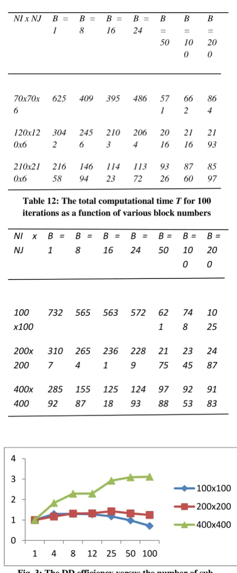
includes the increase of floating point operations induced by grid overlap at interfaces and the CPU time variation generated by DD techniques. In Table 12, we listed the total CPU time distribution over various grid sizes and block numbers running with only one processor. Using this table, the DD efficiency EDD can be calculated, and the result are shown inFig. 3. Note that the DD efficiency can be greater than one, even with one processor. Fig. 3 also shows that the optimum number of sub-domains, which maximizes the DD efficiency
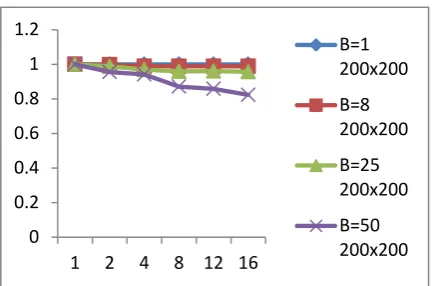
EDD, increases with the grid size. The convergence rate
behavior No / N1, the ratio of the iteration number for the best
sequential CPU time on one processor and the iteration number for the parallel CPU time on n processor, describes the increase in the number of iterations required by the to the serial method. This increase is caused mainly by the deterioration in the rate of convergence with increasing number of processors and sub-domains. Because the best serial algorithm is not known generally, we take the existing parallel program running on one processor to replace it. Now the problem is that how the decomposition strategy affects the convergence rate? The results are summarized in Table 13 and Fig. 4, and Table 14 and Fig. 5. It can be seen that No / N1
decreases with increasing block number and increasing number of processors for given grid size. The larger the grid size, the higher the convergence rate. For a given block number, a higher convergence rate is obtained with less processors. This is because one processor may be responsible for a few domains at each iteration. If some of this sub-domains share some common interfaces, the subsequent blocks to be computed will use the new updated boundary values, and therefore, an improved convergence rate results. The convergence rate is reduced when the block number is large. The reason for this is evident: the boundary conditions propagate to the interior domain in the serial computation after one iteration. But this is delayed in the parallel computation. In addition, the values of variables at the interfaces used in the current iteration are the previous values obtained in the last iteration. Therefore, the parallel algorithm is less “implicit” than the serial one. Despite these inherent short comes. A high efficiency is obtained for large scale problems.
Table 11: The slave computational time TSC, for 100
iterations as a function of various block numbers
NI x NJ B = 1
B = 8
B = 16
B = 24
B = 50
B = 10 0
B = 20 0
70x70x 6
625 409 395 486 57 1
66 2
86 4
120x12 0x6
304 2
245 6
210 3
206 4
20 16
21 16
21 93
210x21 0x6
216 58
146 94
114 23
113 72
93 26
87 60
85 97
Table 12: The total computational time T for 100 iterations as a function of various block numbers
NI x NJ
B = 1
B = 8
B = 16
B = 24
B = 50
B = 10 0
B = 20 0
100 x100
732 565 563 572 62
1 74 8
10 25
200x 200
310 7
265 4
236 1
228 9
21 75
23 45
24 87
400x 400
285 92
155 87
125 18
124 93
97 88
92 53
91 83
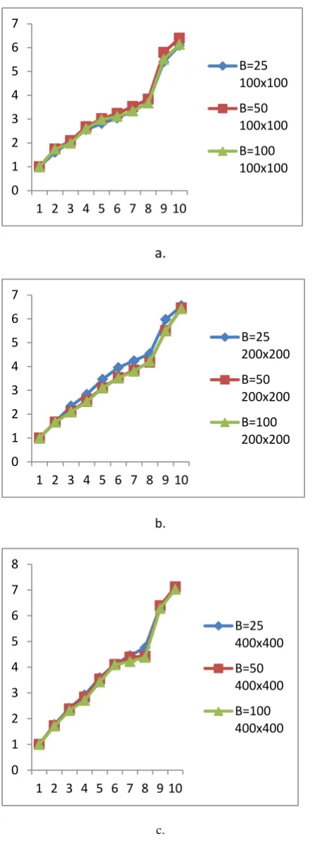
Fig. 3: The DD efficiency versus the number of sub-domains for various meshes.
0 1 2 3 4
1 4 8 12 25 50 100
Table 13: The number of iteration to achieve a given tolerance of 10-3 for a grid of 70x70x6
Table 14: The number of iteration to achieve a given tolerance of 10-2 for a grid of 120x120x6
N B = 1 B = 16 B = 50 B =100
1 2398 2443 2597 2602
2 2398 2451 2628 2724
4 2398 2473 2681 2765
8 2398 2473 2708 2986
12 2398 2473 2701 3032
16 2398 2473 2715 3161
Fig.4: Convergence behavior with domain decomposition for mesh 70x70x6
Fig. 5: Convergence behavior with domain decomposition for mesh 120x120x6
4.4
Total Efficiency
We implemented the serial computations on one of the processors, and calculated the total efficiencies. The total efficiency E(n) for grid sizes 70x70x6 and 120x120x6 have been showed respectively. From Eq. (4.8), we know that the
total efficiency depend on No / N1,
E
par and DD efficiencyEDD since the load balancing is not the real problem here. For
a given grid size and block number, the DD efficiency is constant. Thus, the variation of E(n) with processor number n
is governed by
E
parandN
o/
N
1. When the processor number becomes large, E(n) decreases with n due to the effect of both the convergence rate and the parallel efficiency.5.
CONCLUSIONS
This paper presented a study on the parallelization of 3-D ADI scheme on 3-D Telegraph problem with PVM, on a distributed memory system using SPMD model on a master-slave platform. The system allows a parallel collection of overlapping communication to avoid unnecessary synchronization and to have the impact of parallel convergence. In addition to the use of ease of our platform, compared to other approaches show negligible overhead with effective load scheduling over various mesh sizes, which produce the expected inherent speedups. It was also confirmed that flexible scheduling for the overlapping communication are important, and this is easy on the master-slave platform with SPMD model as seen from the Tables and Figures. The convergence rate depends upon the block numbers and the number of processors for a given grid. For a given number of blocks, the convergence rate increases with decreasing number of processors, and for a given number of processors, it decreases with increasing block number. Computational results obtained have clearly shown the benefits of parallelization. The DD greatly influences the performance of the 3-D ADI scheme on the parallel computers. On the basis of the current parallelization strategy, more sophisticated models can be attacked efficiently.
0 0.2 0.4 0.6 0.8 1 1.2
1 2 4 8 12 16
B=1 200x200 B=8 200x200 B=25 200x200 B=50 200x200
0.8 0.85 0.9 0.95 1 1.05
1 2 4 8 12 16
B=1 100x100 B=8 100x100 B=25 100x100
N B = 1 B = 16 B = 50 B =100
1 2113 2269 2396 2422
2 2113 2327 2518 2564
4 2113 2384 2604 2682
8 2113 2412 2658 2704
12 2113 2412 2661 2712