Development of an Extended Improvement on the Simplified-Bluestein Algorithm

(1)

http://www.sciencepublishinggroup.com/j/com doi: 10.11648/j.com.20170504.11

ISSN: 2328-5966 (Print); ISSN: 2328-5923 (Online)

Development of an Extended Improvement on the

Simplified-Bluestein Algorithm

Amannah Constance Izuchukwu, H. C. Inyiama

Department of Computer Science, University of Nigeria, Nsukka, Nigeria

Email address:

To cite this article:

Amannah Constance Izuchukwu, H. C. Inyiama. Development of an Extended Improvement on the Simplified-Bluestein Algorithm. Communications. Vol. 5, No. 4, 2017, pp. 29-50. doi: 10.11648/j.com.20170504.11

Received: December 21, 2017; Accepted: January 4, 2018; Published: January 31, 2018

Abstract:

This research was designed to develop an extended improvement on the simplified Bluestein algorithm (EISBA). The methodology adopted in this work was iterative and incremental development design. The major technologies used in this work are the numerical algorithms and the C++ programming technologies and the wave concept technology. The C++ served as a signal processing language simulator (SPLS). In the EISBA, the DSP input is encountered first. It is subjected to some numerical processing which included testing for efficiency on the C++ platform. This test platform provided the basis for comparison leading to the desired EISBA. The approach adopted in the study was the re-indexing, decomposing, and simplifying the default SBFFT algorithm. The computing speed of the default algorithms was tested on the C++ platform. The average execution time of the SBFFT was 3.50 seconds. Similarly, the average execution time of the EISBA was 1.74 ms. this result therefore shows that a version of algorithm with computing speed that is faster than that of SBFFT algorithm exist. The algorithms were tested on input block of width 1000 units, and above, and can be implemented on input size of 100 000, and 1000 000 000 without the challenge of storage overflow. The input samples tested in this work was the discretized pulse wave form with undulating shape out of which the binary equivalents were extracted. Other forms of signals may also be tested in the EISBA provided they are interpreted in the digital wave type.

Keywords: Development, Extended, Algorithm, Simplified, Bluestein, Fourier, Transform

1. Introduction

(1). BACKGROUND TO THE STUDY

The most popular digital filters are described and compared in this work. There are only two ways that are common for information to be represented in naturally occurring signals. We will call this information represented in the time domain, and information represented in the frequency domain. Analog signals can also be processed digitally using Digital Signal Processing techniques (DSPTs). To process analog signals digitally, an interface between the analog signal and a digital processor is required. This interface is known as analog-to-digital converter (ADC). The output of the analog-to-digital converter is a digital signal. This digital signal is appropriate for digital processor. The digital signal processor may be a large programmable digital computer or a small microprocessor. In electronics, computer science and mathematics, a digital filter is a system that performs numerical operations on a sampled, discrete-time

(2)

30 Amannah Constance Izuchukwu and H. C. Inyiama: Development of an Extended Improvement on the Simplified-Bluestein Algorithm

at which point, they can be used in testing the algorithms, the existing and the proposed.

STATEMENT OF THE PROBLEM

The speed and scope of transmitting from analog to digital remain issues that need scientific resolution. In view of the foregoing and for effective transition from analog to digital transmission, an efficient computing algorithmic platform is a requirement. This research is therefore designed to develop an efficient numerical algorithm necessary for achieving the speed of processing digital signals in digital computers.

(2). AIM OBJECTIVES OF THE STUDY

The aim of the study is to develop an extended improvement on the simplified Bluestein algorithm. In order to attain this aim, the following objectives were considered;

a) To investigate the simplified Bluestein fast Fourier transforms (SBFFT) algorithm for Digital Signal Processing

b) To design an EISBA for Digital Signal Processing c) To determine the computing speed improvement of the

EISBA for Digital Signal processing

d) To apply warehouse input technology to test and compare the speed of the SBFFT algorithm with the faster Bluestein numerical algorithm

(3). SCOPE OF THE STUDY

This study is restricted to the software approach of DSP-algorithm implementation on a minicomputer or a personal computer. A detailed discussion of hardware, firmware, and DSP chip implementation is beyond the scope of this study.

SIGNIFICANCE OF THE STUDY

The EISBA will provide part of the required directions for transiting from terrestrial analog broadcasting to digital broadcasting. The developed EISBA when implemented will provide an optimized computing framework for simulating signals associated with speech, image, communication, and so on.

2. Related Literature

2.1. Theoretical Framework

Theories related to signal transmission, conversion and processing are discussed, below.

(1). Shannon-Hartley theorem [1]

The Shannon–Hartley theorem [1] states the channel capacity C, meaning the theoretical tightest upper bound on the information rate of data that can be communicated at an arbitrarily low error rate using an average received signal power S through an analog communication channel subject to additive white Gaussian noise of power N:

C = Blog2 (1+ S/N) (1)

where;

C is the channel capacity in bits per second, a theoretical upper bound on the net bit rate (information rate, sometimes denoted I) excluding error-correction codes;

B is the bandwidth of the channel in hertz (passband bandwidth in case of a bandpass signal);

S is the average received signal power over the bandwidth

(in case of a carrier-modulated passband transmission, often denoted C), measured in watts (or volts squared);

N is the average power of the noise and interference over the bandwidth, measured in watts (or volts squared); and

S/N is the signal-to-noise ratio (SNR) or the carrier-to-noise ratio (CNR) of the communication signal to the carrier-to-noise and interference at the receiver (expressed as a linear power ratio, not as logarithmic decibels).

In information theory, the Shannon–Hartley theorem tells the maximum rate at which information can be transmitted over a communications channel of a specified bandwidth in the presence of noise. It is an application of the noisy-channel coding theorem to the archetypal case of a continuous-time analog communications channel subject to Gaussian noise. The theorem establishes Shannon's channel capacity for such a communication link, a bound on the maximum amount of error-free information per time unit that can be transmitted with a specified bandwidth in the presence of the noise interference, assuming that the signal power is bounded, and that the Gaussian noise process is characterized by a known power or power spectral density. The law is named after Claude Shannon and Ralph Hartley.

(2). Noisy Channel Coding Theorem and Capacity [2] The Shannon theorem states that given a noisy channel with channel capacity C and information transmitted at a rate

R, then if R<C there exist codes that allow the probability of error at the receiver to be made arbitrarily small. This means that, theoretically, it is possible to transmit information nearly without error at any rate below a limiting rate, C.

In information theory, the noisy-channel coding theorem (sometimes Shannon's theorem), establishes that for any given degree of noise contamination of a communication channel, it is possible to communicate discrete data (digital information) nearly error-free up to a computable maximum rate through the channel.

Figure 1. Block Diagram of Noisy-Channel Coding Theorem SOURCE: [2].

2.2. History of Digital Signal Processing (DSP)

(3)

possible to predict that traditional analog processing devices such as filters and spectrum analyzers would become digital and result in big improvements for many applications. Acoustic signals such as speech, seismic, and sonar signals were prime candidates for digital processing because of their relatively low bandwidths [2].

According to [2, 3], DSP originated in the 1960s and 1970s when digital computers first came into limelight. Computers were expensive during this era, and DSP was limited to only a few critical applications. Pioneering efforts were made in four key areas: radar and sonar, where national security was at risk; oil exploration, where large amounts of money could be made; space exploration, where the data are irreplaceable; and medical imaging, where lives could be saved. The personal computer revolution of the 1980s and 1990s caused DSP to explode with new applications. Rather than being motivated by military and government needs, DSP was suddenly driven by the commercial marketplace. Anyone who thought they could make money in the rapidly expanding field was suddenly a DSP vendor. DSP reached the public in such products as: mobile telephones, compact disc players, and electronic voice mail.

DSP algorithms have long been run on standard computers, specialized processors called digital signal processor on purpose-built hardware such as application-specific integrated circuit (ASICs). Today there are additional technologies used for digital signal processing including more powerful general purpose microprocessor, field-programmable gate arrays (FPGAs), digital signal controllers and stream processors, among others.

2.3. Fast Fourier Transforms (FFT)

[4, 5] indicated that the FFT revolutionized DSP. It is an elegant and highly effective algorithm that is still the building block used in many state-of-the-art algorithms in speech processing, communications, frequency estimation. There are many different FFT algorithms involving a wide range of mathematics, from simple complex-number arithmetic to group theory and number theory. The DFT is obtained by decomposing a sequence of values into components of different frequencies. An FFT is a way to compute the same result more quickly: computing the DFT of N points in the naive way, using the definition, takes O (N2) arithmetical operations, while an FFT can compute the same DFT in only (NlogN) operations. The difference in speed can be enormous, especially for long data sets where N may be in the thousands or millions. In practice, the computation time can be reduced by several orders of magnitude in such cases, and the improvement is roughly proportional to (NlogN). The FFTs are of great importance to a wide variety of applications, from digital signal processing and solving partial differential equations to algorithms for quick multiplication of large integers. The best-known FFT algorithms depend upon the factorization of N, but there are FFTs with (NlogN) complexity for all N, even for prime N. Many FFT algorithms only depend on the fact that is an N-th primitive root of unity, and thus can be applied to

analogous transforms over any finite field, such as number-theoretic transforms. Since the inverse DFT is the same as the DFT, but with the opposite sign in the exponent and a 1 factor, any FFT algorithm can easily be adapted for it.

Let x0,…, x − 1 be complex numbers. The DFT is defined by the formula

= ∑ = 0, … . − 1 (2)

Evaluating this definition directly requires o operations; there are N outputs XK, and each output requires a

sum of N terms (Johnson and Frigo, 2007). 2.4. Discrete Fourier Transform (DFT)

When a signal is discrete and periodic, continuous Fourier transform is of less importance, [6, 7] instead we use the discrete Fourier transform, (DFT). Suppose our signal is an

where n = 0... N-1, and an = an +JN for all n and j. The

discrete Fourier transform of a, also known as the spectrum of a, is:

! = ∑ " # _$ ₍₃₎ This is commonly written:

!# = ∑ %#&$ (4) Where

% = " (5) And %# for k=0... N-1 are called the Nth roots of unity. They’re called this because, in complex arithmetic, %# = 1 for all k. They are vertices of a regular polygon inscribed in the unit circle of the complex plane (Heckbert, 1998).

2.5. Fast Wavelet Transform (FWT)

The fast wavelet transform (FWT) algorithm is the basic tool for computation with wavelets. The forward transform converts a signal representation from the time (spatial) domain to its representation in wavelet basis. [8, 9] produced a fast wavelet decomposition and reconstruction algorithm. The mallat algorithm for discrete wavelet transform (DWT) is a classical scheme in the signal processing community, known as a two-channel sub-band coder using conjugate quadrature filters or quadrature mirror filters (QMFs).

' ( : = 2+〈- . , ∅ 2+. − 0 〉 (6)

Where ∅ is the scaling function of the chosen wavelet transform; in practice by any suitable sampling procedure under the condition that the signal is highly oversampled, so

2+345 6 : = ∑ ∈;' (_{∅ 7}(8 &9 (7)

(4)

'#+= ∑ @ℎ '+? # (8) A#+ = ∑ @B '+? # (9)

Where '_#+ and A_#+ are viewed as periodic sequences with the period 2 + . The formulae defines an orthogonal mapping: C +? → C +? , converting the coefficients '#+ with = = 1,2, … , 2 +? into the coefficients '#+, A#+ with = = 1,2, … 2 +, and the inverse of Oj is given by the

formulae

'+ = ∑# @# ℎ #'+− = + 1+ ∑# @# B #A+ #? (10)

'+ _{= ∑} _ℎ

# '+ #? # @

# + ∑# @# B # A+ #? (11)

Obviously, given a function f of the form

- = ∑ '#+2

& (

F G2 + _{− = − 1 H +}

& (

# ∑ A#+2

& (

F 2 + _{− = − 1}

& (

# (12)

It can be expressed in the form

- ∑ 'I+ I2

& (JK

F 2 +?I _{− L − 1}

& (JM

I (13)

With

'I+ , L = 1,2, … . , 2 +?I (14)

2.6. Prime-Factor Fast Fourier Transform

The prime-factor algorithm (PFA), also called the Good– Thomas algorithm (1958/1963), is a fast Fourier transform (FFT) algorithm that re-expresses the discrete Fourier transform (DFT) of a size N = N1N2 as a two-dimensional

N1×N2 DFT, but only for the case where N1 and N2 are

relatively prime. These smaller transforms of size N1 and N2

can then be evaluated by applying PFA recursively or by using some other FFT algorithm [10].

Prime factor algorithm (PFA) should not be confused with the mixed-radix generalization of the popular Cooley–Tukey algorithm, which also subdivides a DFT of size N = N1N2 into

smaller transforms of size N1 and N2. The latter algorithm can

use any factors (not necessarily relatively prime), but it has the disadvantage that it also requires extra multiplications by roots of unity called twiddle factors, in addition to the smaller transforms. On the other hand, PFA has the disadvantages that it only works for relatively prime factors (e.g. it is useless for power-of-two sizes) and that it requires a more complicated re-indexing of the data based on the Chinese remainder theorem (CRT). Note, however, that PFA can be combined with mixed-radix Cooley–Tukey, with the former factorizing N into relatively prime components and the latter handling repeated factors.

The prime factor algorithm (PFA) is also closely related to the nested Winograd FFT algorithm, where the latter performs the decomposed N1 by N2 transform via more

sophisticated two-dimensional convolution techniques. Some

older studies therefore also call Winograd's algorithm a PFA FFT. Although the PFA is distinct from the Cooley–Tukey algorithm, Good's 1958 work on the PFA was cited as inspiration by Cooley and Tukey in their famous 1965 paper, and there was initially some confusion about whether the two algorithms were different. In fact, it was the only prior FFT work cited by them, as they were not then aware of the earlier research by Gauss and others. [11, 12].

The PFA involves a re-indexing of the input and output arrays, which when substituted into the DFT formula transforms it into two nested DFTs (a two-dimensional DFT).

2.7. Bruun’s Algorithm

Bruun's algorithm is a fast Fourier transform (FFT) algorithm based on an unusual recursive polynomial-factorization approach, proposed for powers of two by G. Bruun in 1978 and generalized to arbitrary even composite sizes by H. Murakami in 1996. Because its operations involve only real coefficients until the last computation stage, it was initially proposed as a way to efficiently compute the discrete Fourier transform (DFT) of real data. Bruun's algorithm has not seen widespread use, however, as approaches based on the ordinary Cooley–Tukey FFT algorithm have been successfully adapted to real data with at least as much efficiency as possible. Furthermore, there is evidence that Bruun's algorithm may be intrinsically less accurate than Cooley–Tukey in the face of finite numerical precision [13].

Nevertheless, Bruun's algorithm illustrates an alternative algorithmic framework that can express both itself and the Cooley–Tukey algorithm, and thus provides an interesting perspective on FFTs that permits mixtures of the two algorithms and other generalizations.

#= ∑ 0= = = 0, … , − 1. (15)

For convenience, let us denote the N root of unity by N 0 = 0, … , − 1 :

N = (16) And define the polynomial x (z) whose coefficients are xn

O ∑ O . (17) The DFT can then be understood as a reduction of this polynomial; that is Xk is given by

#= N# = O PQA O − N (18)

Where mod denotes the polynomial remainder operation. The key to fast algorithms like Bruun’s or cooley-Tukey comes from the fact that one can perform this set of N

remainder operations in recursive stages.

2.8. Complex DSP Versus Real DSP

(5)

programs merely rearrange stored data. This means that computers designed for business and other general applications are not optimized for algorithms such as digital filtering and Fourier analysis. Digital Signal Processors are microprocessors specifically designed to handle Digital Signal Processing tasks [14].

Complex numbers are an extension of the ordinary numbers used in everyday math. They have the unique property of representing and manipulating two variables as a single quantity. This fits very naturally with Fourier analysis, where the frequency domain is composed of two signals, the real and the imaginary parts. Complex numbers shorten the equations used in DSP, and enable techniques that are difficult or impossible with real numbers alone [14, 15].

Digital Signal Processing (DSP) is a vital tool for scientists and engineers, as it is of fundamental importance in many areas of engineering practice and scientific research. The “alphabet” of DSP is mathematics although most practical DSP problems can be solved by using real number mathematics, there are many others which can only be satisfactorily resolved or adequately described by means of complex numbers. If real number mathematics is the language of real DSP, then complex number mathematics is the language of complex DSP. In the same way that real numbers are a part of complex numbers in mathematics, real DSP can be regarded as a part of complex DSP [15].

2.9. Complex Representation of Signals and Systems

Complex numbers offer a compact representation of the most often-used waveforms in signal processing – sine and

cosine waves [15, 16]. The complex number representation of sinusoids is an elegant technique in signal and circuit analysis and synthesis, applicable when the rules of complex math techniques coincide with those of sine and cosine functions. Sinusoids are represented by complex numbers; these are then processed mathematically and the resulting complex numbers correspond to sinusoids, which match the way sine and cosine waves would perform if they were manipulated individually. The complex representation technique is possible only for sine and cosine waves of the same frequency, manipulated mathematically by linear systems.

All naturally-occurring signals are real; however in some signal processing applications it is convenient to represent a signal as a complex-valued function of an independent variable. For purely mathematical reasons, the concept of complex number representation is closely connected with many of the basics of electrical engineering theory, such as voltage, current, impedance, frequency response, transfer-function, Fourier and z-transforms, and so on. Complex DSP has many areas of application, one of the most important being modern telecommunications, which very often uses narrowband analytical signals; these are complex in nature [16].

2.10. Complex DSP Applications in Telecommunications

Telecommunication systems very commonly require processing to occur in real time, adaptive complex filtering being amongst the most frequently-used complex DSP techniques. When multiple communication channels are to be manipulated simultaneously, parallel processing systems are indicated [16, 17]. An efficient Adaptive Complex Filter Bank (ACFB) scheme is presented here, together with a short exploration of its application for the mitigation of narrowband interference signals in MIMO (Input Multiple-Output) communication systems. DSP is making a significant contribution to progress in many diverse areas of human endeavour – science, industry, communications, health care, security and safety, commercial business, space technologies etc. Based on powerful scientific mathematical principles, complex DSP has overlapping boundaries with the theory of, and is needed for many applications in, telecommunications. Modern telecommunications very often uses narrowband signals, such as NBI (Narrowband Interference), RFI (Radio Frequency Interference), and so on. These signals are complex by nature and hence it is natural for complex DSP techniques to be used to process them [16, 17, 18]

3. Methodology

The design model adopted in this work was the Reconstructive Iterative Development Model (RIDM). The procedure itself consists of the initialization step, the iteration step, and the Project Control List. The initialization step creates a base version of the system. The goal for this initial implementation is to create a product to which the user can react. It should offer a sampling of the key aspects of the problem and provide a solution that is simple enough to understand and implement easily. To guide the iteration process, a project control list is created that contains a record of all tasks that need to be performed. It includes such items as new features to be implemented and areas of redesign of the existing solution. The control list is constantly being revised as a result of the analysis phase.

(6)

Figure 2. Reconstructive Iterative Development Model.

3.1. An Overview of the Existing System

The existing system is generally referred to as Simplified Bluestein Fast Fourier Transforms (SBFFT) algorithm.

The SBFFT Algorithm

3 4 1/ 2

( ) ( 2 / ) ( )

X k =esp j

π

N K n _x n N− _ (19)

3.2. The Proposed System

The proposed system is Extended Improvement on the Simplified-Bluestein Algorithm (EISBA). The proposed system works with digital signal inputs. These inputs are collected from warehouse. The essence is to test the (EISBA) with a view to determining its computing speed in comparison with SBFFT algorithm.

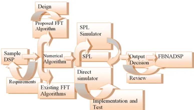
3.3. Architecture of the Proposed System

The architecture of the proposed system as shown in figure 3 below describes all the steps and stages necessary for the development of the proposed EISBA for digital signal processing. The architecture clearly illustrates the process and procedures of the iterative development model adopted in this research. The architecture begins with the DSP data input (requirement step in the iterative model), followed by the determination of the present and proposed algorithms (the design step of the iterative model), followed by the comparison of both algorithms (the implementation and test step of the iterative model) and climaxed with the output and decision state (the review step of the iterative model). The output and decision stage eventually leads to the desired and expected result of the research, which is the EISBA.

(7)

3.4. Design of the Proposed System

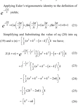
The proposed algorithm results from further decomposition, re-indexing and simplification of the SBFTT algorithm. The procedure is outlined below:

3 4 1/ 2

( ) ( 2 / ) ( )

X k =esp j

π

N K n _x n N− _ [SBFFT] (20)

Applying Euler’s trigonometric identity to the definition of 2 −j N

e

π yields; 2

2 2 2 2

1 0 1

j

N _Cos _jSin _Cos _jSin

N N N N

e

π _π _π _π _π − −  −  =  +  = − = + =     (21)

Simplifying and Substituting the value of eq (20) into eq

(19) and x (n) = 1( 2 2

(

)

2

2 n k n k k

 

+ − −

 

  we have;

(

) (

)

2

2 1

2 2 2

2 1 ( ) 2 j k N

X k n

_e

n k n k k

π 

− _− _ _ _

+ = _ + − − _ (22)

(

)

2 1 2 2 2 2 1 1 ( 2 k

n k n k k

  −  

  

= _ + − − _ (23)

= 1( 2 2 2 2 2

2 n k n k nk k

 

+ − + −

 

  (24)

= 1(2 2 2 )

2 k nk k

 

−

 

  (25)

= _k2−nk_ (26)

Eq (26) shows that there is no variance in the signals going through platform. By convolution principle, the introduction of the delta function yields the same signal; hence eq (26) can be expressed as:

(

)

( ) ( )

X k+ =n Y k+ ×n δ x (27)

Where Y k( + =n) 2 (n2+k2)=2nk (28)

Eqn (25) is the resulting algorithm with one exponentiation, one product and one subtraction. This is a minimized version of the SBFFT algorithm which has four exponentiations and five products. Such reduction in the number of operators can account for speed of the generated algorithm even as their implementation reveals.

3.5. Implementation Architecture

The various components of the software modules and

sub-modules of the proposed system are clearly described in figure 4 below.

Figure 4. Implementation Architecture of the Proposed System.

In figure 4 above, the main modules of the system include FFT algorithms and the proposed algorithm. Each of the main modules consists of sub-modules. The sub-modules of the SBFFT algorithm is first iteration and the second iteration. The sub-module of the proposed algorithm is semi-EISBA. The sub-modules are implemented (tested) leading to the determination of the semi-EISBA and the subsequent EISBA, the expected result of the system.

4. Discussion of Results

The result of this study shows that we can have faster numerical algorithms other than the SBFFT algorithm for the processing of digital signals. The EISBA resulted from the re-indexing and modification of the SBFFT algorithm. The authors by this result therefore succeeded in developing an algorithm that is faster than the SBFFT algorithm. The speed advantage of the developed algorithm is significant enough that there is a necessary shift of efficiency rate from seconds to milliseconds. In favour of this study, the developed algorithm is called EISBA. The computing speed of the default algorithms was tested on the C++ platform.

4.1. Comparison of the Existing System with the Proposed System

The proposed system when compared with the existing system is of more efficiency than the existing system. Table 1 below illustrates the comparison more succinctly.

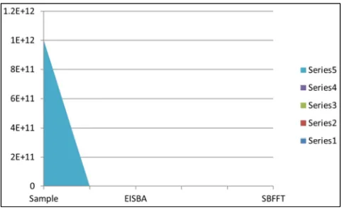
Table 1. Output comparison of the sbfft algorithm with the eisba.

Number Numerical Algorithms

SBFFT (Sec) EISBA (ms) % Improvement

N=1000 3.50 1.74 77.28%

N=1000 000 1.75 79.28%

(8)

Communications 2017; 5(4): 29-50 35

Figure 5. Graph of EISBA against SBFFT Algorithm.

In Figure 5 above, the triangular shape of the graph is expanded horizontally indicating the direction of the SBFFT algorithm while the vertical contraction represents the EISBA. It simply explains that the greater the sample, the smaller the operation time of the EISBA and the slower the computing speed of the SBFFT algorithm.

5. Summary and Conclusion

5.1. Summary

In search of a faster algorithm, the established default algorithm was subjected to re-indexing, decomposition, and simplification. The re-indexing stage was to define and substitute each parameter variable in the original SBFFT algorithm. This effort redefined the apparent structure of SBFFT algorithm. The decomposition process explored the impact of

the trigonometric identity. Applying this trigonometric identity into the re-indexed algorithm expanded the algorithm downward making room for further simplification. This downsized algorithm provided the direction of the expected EISBA with the elimination of non-unique arithmetic operators. The presence of the non-unique operators contributed to the constraints of the default SBFFT algorithm. Their absence or elimination contributed to the efficiency of the new algorithm. The simplification effort adjusted the number of multiplication, exponentiation, addition, and subtraction operations and operators. At this stage, the algorithm became narrower, simpler, and of course faster also.

The three processes described above yielded the EISBA that when tested on the C++ platform, proved faster than the default SBFFT algorithm. The speed advantage of the EISBA was as high 1.74 ms. The index frequency, K is the speed factor in this study. The K factor determines the speed of the algorithm while the signal index, n determines the quantum of the signal.

5.2. Conclusion

The result of this study is certainly going to enhance the computing speed of digital signals. The developed algorithms are basically recommended for the processing of digital signals and not analog signals. However, it can also be used for analog signals only when they are converted to digital signals. The algorithms were tested on input block width of 1000, and above, and can be implemented on input size of 100 000, and 1000 000 000 without the challenge of storage overflow.

Appendix

Appendix A: Source Code

• #include <iostream> • #include <list> • #include <cstdlib> • using namespace std; • int main()

• {

• int choice, item; • list<int> lt;

• list<int>::iterator it; • while (1)

• {

• cout<<"\n---"<<endl;

• cout<<"Sorting Containers Implementation in Stl"<<endl; • cout<<"\n---"<<endl;

• cout<<"1.Insert Element into the List"<<endl; • cout<<"2.Display Sorted Elements"<<endl; • cout<<"3.Exit"<<endl;

• cout<<"Enter your Choice: "; • cin>>choice;

• switch(choice) • {

(9)

• cout<<"Enter the element to be inserted: "; • cin>>item;

• lt.push_back(item); • break;

• case 2:

• lt.sort();

• cout<<"Elements of Sorted List: ";

• for (it = lt.begin(); it != lt.end(); ++it) • cout <<" "<< *it;

• cout << endl; • break;

• case 3: • exit(1); • break; • default:

• cout<<"Wrong Choice"<<endl; • }

• }

• return 0;

• }

#include <iostream> • #include <stack> • #include <string> • #include <cstdlib> • using namespace std; • int main()

• {

• stack<int> st; • int choice, item; • while (1)

• {

• cout<<"\n---"<<endl; • cout<<"Stack Implementation in Stl"<<endl; • cout<<"\n---"<<endl;

• cout<<"1.Insert Element into the Stack"<<endl; • cout<<"2.Delete Element from the Stack"<<endl; • cout<<"3.Size of the Stack"<<endl;

• cout<<"4.Top Element of the Stack"<<endl; • cout<<"5.Exit"<<endl;

• case 1:

• cout<<"Enter value to be inserted: "; • cin>>item;

• st.push(item); • break;

• case 2:

• item = st.top(); • st.pop();

• cout<<"Element "<<item<<" Deleted"<<endl; • break;

• case 3:

(10)

• break; • case 4:

• cout<<"Top Element of the Stack: "; • cout<<st.top()<<endl;

• break; • case 5: • exit(1); • break; • default:

• }

• return 0;

• }

• #include <iostream> • #include <map> • #include <string> • #include <cstdlib> • using namespace std; • int main()

• {

• map<char,int> mp;

• map<char, int>::iterator it; • int choice, item;

• char s; • while (1) • {

• cout<<"\n---"<<endl; • cout<<"Map Implementation in Stl"<<endl; • cout<<"\n---"<<endl;

• cout<<"1.Insert Element into the Map"<<endl; • cout<<"2.Delete Element of the Map"<<endl; • cout<<"3.Size of the Map"<<endl;

• cout<<"4.Find Element at a key in Map"<<endl; • cout<<"5.Dislplay by Iterator"<<endl;

• cout<<"6.Count Elements at a specific key"<<endl; • cout<<"7.Exit"<<endl;

• case 1:

• cout<<"Enter the key: "; • cin>>s;

• mp.insert(pair<char,int>(s ,item)); • break;

• case 2:

• cout<<"Enter the mapped string to be deleted: "; • cin>>s;

• mp.erase(s); • break;

• case 3:

(11)

• cout<<"Enter the key at which value to be found: "; • cin>>s;

• if (mp.count(s) != 0)

• cout<<mp.find(s)->second<<endl; • else

• cout<<"No Element Found"<<endl; • break;

• case 5:

• cout<<"Displaying Map by Iterator: ";

• for (it = mp.begin(); it != mp.end(); it++) • {

• cout << (*it).first << ": " << (*it).second << endl; • }

• cout<<"Enter the key at which number of values to be counted: "; • cin>>s;

• cout<<mp.count(s)<<endl; • break;

• case 7:

• exit(1); • break; • default:

• }

• return 0;

• }

• #include <iostream> • #include <stack> • #include <string> • #include <cstdlib> • using namespace std; • int main()

• {

• stack<int> st; • int choice, item; • while (1)

• {

• cout<<"\n---"<<endl; • cout<<"Stack Implementation in Stl"<<endl; • cout<<"\n---"<<endl;

• cout<<"1.Insert Element into the Stack"<<endl; • cout<<"2.Delete Element from the Stack"<<endl; • cout<<"3.Size of the Stack"<<endl;

• cout<<"4.Top Element of the Stack"<<endl; • cout<<"5.Exit"<<endl;

• case 1:

(12)

• st.push(item); • break;

• case 2:

• item = st.top(); • st.pop();

• cout<<"Element "<<item<<" Deleted"<<endl; • break;

• case 3:

• cout<<"Size of the Queue: "; • cout<<st.size()<<endl;

• cout<<"Top Element of the Stack: "; • cout<<st.top()<<endl;

• break; • case 5: • exit(1); • break; • default:

• }

• return 0;

• }

• #include <iostream> • #include <forward_list> • #include <string>

• #include <cstdlib> • using namespace std; • int main()

• {

• forward_list<int> fl, fl1 = {5, 6, 3, 2, 7}; • forward_list<int>::iterator it;

• int choice, item; • while (1)

• {

• cout<<"\n---"<<endl;

• cout<<"Forward_List Implementation in Stl"<<endl; • cout<<"\n---"<<endl;

• cout<<"1.Insert Element at the Front"<<endl; • cout<<"2.Delete Element at the Front"<<endl; • cout<<"3.Front Element of Forward List"<<endl; • cout<<"4.Resize Forward List"<<endl;

• cout<<"5.Remove Elements with Specific Values"<<endl; • cout<<"6.Remove Duplicate Values"<<endl;

• cout<<"7.Reverse the order of elements"<<endl; • cout<<"8.Sort Forward List"<<endl;

• cout<<"9.Merge Sorted Lists"<<endl; • cout<<"10.Display Forward List"<<endl; • cout<<"11.Exit"<<endl;

• case 1:

(13)

• fl.push_front(item); • break;

• case 2:

• item = fl.front(); • fl.pop_front();

• cout<<"Element "<<item<<" deleted"<<endl; • break;

• case 3:

• cout<<"Front Element of the Forward List: "; • cout<<fl.front()<<endl;

• cout<<"Enter new size of Forward List: "; • cin>>item;

• if (item <= fl.max_size()) • fl.resize(item);

• else

• fl.resize(item, 0); • break;

• case 5:

• cout<<"Enter element to be deleted: "; • cin>>item;

• fl.remove(item); • break;

• case 6:

• fl.unique();

• cout<<"Duplicate Items Deleted"<<endl; • break;

• case 7:

• fl.reverse();

• cout<<"Forward List reversed"<<endl; • break;

• case 8:

• fl.sort();

• cout<<"Forward List Sorted"<<endl; • break;

• case 9:

• fl1.sort(); • fl.sort(); • fl.merge(fl1);

• cout<<"Forward List Merged after sorting"<<endl; • break;

• case 10:

• cout<<"Elements of Forward List: ";

• for (it = fl.begin(); it != fl.end(); it++) • cout<<*it<<" ";

• cout<<endl; • break; • case 11: • exit(1); • break;

• default:

• }

• return 0;

(14)

• #include <iostream> • #include <algorithm> • #include <vector> • using namespace std; • int main ()

• {

• int first[] = {5,10,15,20,25}; • int second[] = {50,40,30,20,10}; • vector<int> v(10);

• vector<int>::iterator it; • sort (first, first + 5); • sort (second, second + 5);

• it = set_difference(first, first + 5, second, second + 5, v.begin()); • v.resize(it - v.begin());

• cout << "The difference has " << (v.size()) << " elements: "<<endl; • for (it = v.begin(); it != v.end(); ++it)

• cout<< *it<<" "; • cout <<endl;

• return 0;

• }

• #include <iostream> • #include <algorithm> • #include <vector> • using namespace std; • int main ()

• {

• int f[] = {5,10,15,20,25}; • int s[] = {50,40,30,20,10}; • vector<int> v(10);

• vector<int>::iterator it; • sort (f, f + 5);

• sort (s, s + 5);

• it = set_symmetric_difference(f, f + 5, s, s + 5, v.begin()); • v.resize(it - v.begin());

• cout<<"The symmetric difference has "<< (v.size())<< " elements: "<<endl; • for (it = v.begin(); it != v.end(); ++it)

• cout<< *it<<" "; • cout <<endl;

• return 0;

• }

#include <iostream> • #include <algorithm> • using namespace std;

• void display(int a[], int n)

• {

• for(int i = 0; i < n; i++) • {

• cout<<a[i]<<" "; • }

• cout<<endl;

• }

• int main ()

• {

• int num, i;

(15)

• cin>>num;

• int myints[num];

• for (i = 0; i < num; i++) • {

• cout<<"Enter "<<i + 1<<" element: "; • cin>>myints[i];

• }

• sort (myints, myints + num);

• cout << "The "<<num<<"! possible permutations with "; • cout<<num<<" elements: "<<endl;

• do • {

• display(myints, num); • }

• while (next_permutation(myints, myints + num)); • return 0;

• }

#include <iostream> • #include <algorithm> • using namespace std;

• void display(int a[], int n)

• {

• for(int i = 0; i < n; i++) • {

• cout<<a[i]<<" "; • }

• cout<<endl;

• }

• int main ()

• {

• int num, i;

• cout<<"Enter number of elements to be inserted: "; • cin>>num;

• int myints[num];

• for (i = 0; i < num; i++) • {

• cout<<"Enter "<<i + 1<<" element: "; • cin>>myints[i];

• }

• sort (myints, myints + num); • reverse (myints, myints + num);

• cout << "The "<<num<<"! possible permutations with "; • cout<<num<<" elements: "<<endl;

• do • {

• display(myints, num); • }

• while (prev_permutation(myints, myints + num)); • return 0;

• }

#include <iostream.h> #include <ctype.h> #include <stdlib.h>

(16)

const Bool TRUE = 1; const Bool FALSE = 0;

void readLetter(char&);

int computeCorrespondingDigit(char);

Bool doOneLetter(); //returns flag saying whether you should quit

void main () {

Bool flag = FALSE;

while (!flag) {

flag = doOneLetter(); }

}

int exitLetter (char c) {

return ((c == 'Q') || (c == 'Z')); }

Bool doOneLetter() { char l;

int i;

readLetter(l); // returns upper case letter if (exitLetter(l)) {

cout << "Quit." << endl; return(TRUE);

} else {

i = computeCorrespondingDigit(l);

cout << "The letter " << l << " corresponds to " << i << " on the telephone" << endl;

return(FALSE); }

}

int computeCorrespondingDigit (char l) { switch (l) {

case 'A' : case 'B' : case 'C' : return(2); case 'D' : case 'E' : case 'F' : return(3); case 'G' : case 'H' : case 'I' : return(4); case 'J' : case 'K' :

(17)

• int main()

• {

• vector<int> ss;

• vector<int>::iterator it; • int choice, item;

• while (1) • {

• cout<<"\n---"<<endl; • cout<<"Vector Implementation in Stl"<<endl; • cout<<"\n---"<<endl;

• cout<<"1.Insert Element into the Vector"<<endl; • cout<<"2.Delete Last Element of the Vector"<<endl; • cout<<"3.Size of the Vector"<<endl;

• cout<<"4.Display by Index"<<endl; • cout<<"5.Dislplay by Iterator"<<endl; • cout<<"6.Clear the Vector"<<endl; • cout<<"7.Exit"<<endl;

• case 1:

• ss.push_back(item); • break;

• case 2:

• cout<<"Delete Last Element Inserted:"<<endl; • ss.pop_back();

• cout<<"Size of Vector: "; • cout<<ss.size()<<endl; • break;

• case 4:

• cout<<"Displaying Vector by Index: "; • for (int i = 0; i < ss.size(); i++) • {

• cout<<ss[i]<<" "; • }

• cout<<endl; • break; • case 5:

• cout<<"Displaying Vector by Iterator: "; • for (it = ss.begin(); it != ss.end(); it++) • {

• cout<<*it<<" "; • }

• cout<<endl; • break; • case 6:

• ss.clear();

• cout<<"Vector Cleared"<<endl; • break;

(18)

• default:

• }

• return 0;

• }

Appendix B

(19)

(20)

(21)

Appendix C

Dft Analog Signals (Adapted From [10, 11, 12, 13]).

1. the sine graph starts at zero

2. it repeats itself every 360 degrees (or 2 pi)

3. y is never more than 1 or less than -1 (displacement from the x-axis is called the amplitude) 4. a sin graph 'leads' a cos graph by 90 degrees

(22)

References

[1] Mathuranathan v. (2008). Channel Capacity & Shannon’s theorem – demystified. Retrieved 14/04/2017 from http://www.gaussianwaves.com/2008/04/channel-capacity/ Fast wavelet

transformlink.springer.com/chapter/10.1007%2F978-3-319- 22075-8_7by J Gomes - 2015 - Related articles.

[2] Slot L. and Zur S. (2015). Shannon's Noisy-Channel Coding Theorem. Retrieved 12/03/2017 from

http://homepages.cwi.nl/~schaffne/courses/infcom/2014/prese ntations/Luca s_Sebastian_NoisyChannelCoding.pdf.

[3] Fraser, D. (1989). Interpolation by the FFT Revisited An Experimental Investigation, IEEE Transactions on Acoustics, Speech, and Signal Processing, (37) 5, pp. 665-675.

[4] Matthew, P. D. (2000). Efficient Digital Filters, IEEE Transactions on Acoustics, Speech and Signal Processing, ASSP-.

[5] Sanjit, K. M. (2001). Digital Signal Processing: A Computer Approach, McGraw-Hill, New York.

[6] Yin, L. G., Agiieswari, K. R., (2005). Evaluation of DSP Based Numerical Relay for Over Current Protection Centre for Communication Service Convergence Technologies (CCSCT). Department of Electronics and Communication Engineering, Beijing China.

[7] Areva, T. D. (1995). Network Protection and Automation Guide. Prentice Hall. New Jersey.

[8] http://www.jstor.org/stable/3680137 Accessed: 30/07/2012 23:37.

[9] Good, I. J. “The interaction algorithm and practical fourier analysis”. Journal of the royal statistical society, series B 20 (2): 361–372 JSTOR 2983896, 1958.

(https://www.jstor.or/state/2983896). Addendum, ibid. 22 (2), 375 (1960).

[10] Thomas, L. H. (1963). Using Computers to solve problems in Physics. Applications of Digital computers. Bostom: Ginn. [11] Pavan Kumar K. M., Priya Jain, Ravi Kiran S, Rohith N.,

Ramamani K. FFT Algorithm: A Survey. The International Journal of Engineering and Science (IJES) Volume 2 Issue 4 pages 22-26, 2013 ISSN (e): 2319-1813.

[12] Standard 982. 1 – 1988. Piscataway, N. J: IEEE. Jessica Keyes software Engineering productivity handbook. Windcrest/MC. [13] Pfleeger, S. L. and C. McGowam 1990. Software metrics in

the process maturity framework. Journal of Systems Software. 12:255-261.

[14] https://www.researchgate.net/publication/221920249 Complex_Digital_Signal_Processing_in_T

elecommunications [accessed May 29, 2017].

[15] Godsill S. (2014). 3F3 Digital Signal Processing (DSP). Retrieved 27/05/2017 from https://www- sigproc.eng.cam.ac.uk/foswiki/pub/Main/3F3/3F3__Digital_S ignal_Processing_(DSP)_2015_1 -49.pdf.

[16] Drago D. (2012). Theory of Signal. Retrieved 14/06/2017 from http://www.informatics.buzdo.com/p030-signal- theory.htm Heckbert P. (1998). Fourier Transforms and the Fast Fourier Transform (FFT) Algorithm. Retrieved 02/05/2017 from

https://www.cs.cmu.edu/afs/andrew/scs/cs/15-463/2001/pub/www/notes/fourier/fourier.pdf.

[17] Vladimir, P. and Zlatka, N., Georgi, I., Miglen, O., (2011). Complex Digital Signal Processing in Telecommunications: Applications of Digital Signal Processing, Dr. Christian Cuadrado-Laborde (Ed.), 307-406.