http://www.sciencepublishinggroup.com/j/ijdsa doi: 10.11648/j.ijdsa.20190502.11
ISSN: 2575-1883 (Print); ISSN: 2575-1891 (Online)
Power of Simulation Extrapolation in Correction of
Covariates Measured with Errors
Joseph Njuguna Karomo
*, Samuel Musili Mwalili, Anthony Wanjoya
Department of Statistics and Actuarial Sciences, Jomo Kenyatta University of Agriculture and Technology, Nairobi, Kenya
Email address:
*
Corresponding author
To cite this article:
Joseph Njuguna Karomo, Samuel Musili Mwalili, Anthony Wanjoya. Power of Simulation Extrapolation in Correction of Covariates Measured with Errors. International Journal of Data Science and Analysis. Vol. 5, No. 2, 2019, pp. 13-17. doi: 10.11648/j.ijdsa.20190502.11
Received: April 18, 2019; Accepted: May 21, 2019; Published: June 5, 2019
Abstract:
Statistics is one of the most vibrant disciplines where research is inevitable. Most researches in statistics are concerned with the measurement of values of variables in order to make valid conclusions for decision making. Often, researchers do not use the exact values of the variables since it’s difficult to establish the exact value of variables during data collection. This study aimed at using simulation studies to ascertain the power of Simulation Extrapolation (SIMEX) in correcting the bias of coefficients of a logistic regression model with one covariate measured with error. The corrected coefficient values of the model can then be used to predict the exact values of the explanatory variable. The Mean Square Error and the coverage probability were used to test the adequacy of the different model's estimates. The study showed that the use of SIMEX with the quadratic fitting method would give significantly good estimates of the model’s predictors’ coefficients. For further studies, the researcher recommends the study to be done using other models and with multiple covariates measured with errors.Keywords:
Simulation Extrapolation, SIMEX, Measurement Errors, Berkson Error, Naive Estimator, Bias1. Introduction
Logistic regression is a widely used tool in the analysis of the data when the response variable is binary in nature (for example the presence or absence of a disease). The response variable is explained by the different explanatory variables in the model. The different coefficients on the explanatory variables are the gradients with respect to the variables they are associated with. The role of regression analysis is to correctly estimate these coefficients. Correct estimates of the model coefficients can only be gotten when the explanatory variables are measured without errors. However, the normal assumption that the explanatory variables have no error does not always hold water. When these explanatory variables are measured with errors, then the gradient estimates are biased. The gradient estimate for a covariate measured with error will be;
∗ (1)
Fuller refers to as the reliability ratio [1].
Various methods have been proposed by different researchers to correct this bias that is associated with measurement errors of the covariates. Cook and Stefanski explained the simulation extrapolation (SIMEX) method which is one of such methods [2]. This study used simulation studies by simulating a true model then introducing errors in one of the covariates to come up with a naive model that was later used in Simulation Extrapolation procedure. The researcher used the R - SIMEX library for extrapolation.
2. Methodology
2.1. Measurement Errors
Classical measurement errors. Freedman et al. claimed that the fundamental difference between the two kinds of measurement errors is based on the distribution assumed by the errors [3].
2.1.1. Classical Error Model
According to Stefanski and Cook, Classical error model assumes a distribution for the observed values given the true values ( | ) [4]. This model also assumes that measurement errors are independent of the true values and the explanatory variable X is incorrectly recorded by W. Babanezhad, expressed the classical model as;
+ (2) Where U is the measurement error and is assumed to be independent of X [5].
2.1.2. Berkson Error Model
The basic assumption in Berkson error model is that the model assumes a distribution for the true values given the observed values ( | ) and that measurement error is always independent of the observed explanatory variable W. Babanezhad, expressed the Berkson model as follows [5];
+ (3) Rudemo, Ruppert and Streibig suggested that Berkson error model has proved to be very efficient in medical and agriculture studies [6].
2.2. Measurement Error in a Logistic Regression Model
According to Stefanski, logistic regression is one of the non-linear models that are often concerned with measurement error [7]. We consider a logistic regression model for the dependence of a binary response Y with the scalar predictor X in which;
Pr( 1| ) ( + ) (4) Where;
H(θ) !" (#$) (5)
Given the data set ( , ), 1,2, … , ( the maximum likelihood estimator needs numerical maximization. We suppose that the latent variable is unobservable, but the quantity + is observed. Since the MLE’s don’t have close-form expression, the effect of replacing X with W in logistic regression is not easily determined, though Stefanski claims that the estimate of is attenuated as in the case of linear regression [7].
In logistic regression, estimation when the measurement error is normally distributed proceeds under the assumption that variance of the error is known or it is independently estimable, for example, replicate measurement.
Next, we consider the functional version of logistic measurement error model with errors U which are normally distributed with known variance )*+ . Here the density function of ( , ) is given by;
,-.(/, 0| , , ) { ( + )}3{1 − ( + )} #3 5∅ 78#95:; (6)
Where ∅() is the standard normal density function.
2.3. Simulation Extrapolation (SIMEX)
Cook and Stefanski were the first researchers to suggest the SIMEX method and it was developed further by Stefanski and Cook and Carroll and Küchenhoff [4, 8]. Shang explains the simulation extrapolation (SIMEX) method as a technique used for correction of measurement error through simulation [9]. In the lines of Weeding, this method is used when the measurement error variance can be accurately estimated from replicated measurement or from validation data or the variance is already known [10]. The method further assumes that there exists an estimator which is consistent when all variables are measured without error. Such an estimator is referred to as the naive estimator when it is used despite the measurement error.
Küchenhoff, Mwalili, and Lesaffre note that SIMEX utilizes the relationship of measurement error variance )<+ to the bias of the effect estimators while disregarding the measurement error [11]. As a result, SIMEX estimator is obtained by adding additional measurement error to the already observed data in the resampling stage, establishing a relation of the error-induced bias against the variance of the added measurement error and extrapolating back to a case where no measurement error is present. We then define the
following function;
)<+→ ∗()<+) =: ?()<+) (7)
Where ∗ is the limiting value of the naive estimator as the sample size increases to infinity. The result of consistency is that ?(0) = . Mwalili suggests that more often ?()<+)
declines in its absolute value as )<+ increases [12]. G() <+)
matches to the attenuation of the projected effect induced by the measurement error. The SIMEX method is built on the parametric estimation of the function ?()<+) ≈ ?()<+; D) for
instance, in a quadratic approximation;
()<+, Γ) = F F )
<++ F+()<+)+ (8)
2.4. SIMEX in Simple Linear Regression
SIMEX method is best illustrated by the use of simple linear measurement error regression model. For illustration purposes, we consider the following model;
G( | ) = + (9)
We also consider that ∗= + )* instead of X is
observed where U is normally distributed with mean zero and variance 1 and that the measurement error variance )<+ is
∗ = = (10)
Fuller refers to = to as reliability ratio [1]. )+
denotes the variance of . Now, consider adding by simulation, additional error with mean zero and variance )<+H
to ∗resulting in ∗∗, for fixed H ≥ 0 so that the variance of
∗∗ is )
<++ )<+H = (1 + H))<+ Then, an ordinary least squares
regression of Y on ∗∗consistently estimates the following
quantity.
∗ ∗(H) =
( J) (11)
We observe that at H = −1, ∗∗(H) = i.e, ∗∗(−1) =
which, in this case, will represent a situation with no measurement error. Hence, the rule of thumb is to fit a regression model of ∗∗(H) against H and then extrapolate the graph back to where H = −1.
Hasan et al. pointed out that without loss of generality, for any set of data, the SIMEX method uses simulation to add more measurement error with a variance of )<+H to the error susceptible variable [13]. As a result, the measurement error then becomes (1 + H))<+ which will lead to an estimator that converges to ?((1 + H))<+) for naive estimation. A repetition of this simulation procedure for a fixed grid of H’M gives an estimator DN of the parameters of ?()<+, Γ) by least squares. During the extrapolation stage, the function ?()<+; D) is extrapolated to 0. SIMEX estimator is demarcated by
?(0; DN) that is, setting H = −1 in ?((1 + H))<+). For cases where ?()<+; D) is a good estimate to the function ?()<+), then Mwalili claims that SIMEX criteria are approximately consistent [12].
2.5. Jackknife Variance Estimation
One drawback of SIMEX procedure is that the error variance should be known or it is independently and correctly estimable for instance using the replicate measurement. A study by Tsamardinos et al. gives more insight into the jackknife variance estimation procedure which is otherwise referred to as a leave - one - out method [14]. It is an alternative to other variance estimation procedures such as bootstrap method and the delta method. According to Shao and Dongsheng the idea in jackknife variance estimation is to sequentially delete one observation from the dataset and then calculating the estimator ON n times [15]. This implies that for a sample of size n we have ( jackknife estimates. Suppose we have n observations, we compute n estimates by sequentially omitting one observation from the dataset and then estimating ON on the ( − 1 observations that remained. The building blocks of a jackknife variance estimate are basically the n differences [4]. i.e.
∆ = ON(Q# ), ( ) − ON(Q# ), (. ); = 1, 2, 3, … , ( . The normal jackknife variance estimate is Q#Q ∑ ∆QT + . Using ( jackknife estimates; ON( ), ON(+), ON(U), … , ON(Q), We then estimate the standard error of the estimator as;
MV[ = \WXYZ Q#Q ∑ (ON( )QT − ON̅(.))+ (12)
3. Results and Discussions
3.1. Data Simulation
To explore the power of SIMEX for error correction, the researcher simulated two variables (x.true – random exponential values and z – normal random variables) each with size 200. These two variables were used to come up with a logistic regression with variable y denoting the response variable with a binary outcome. A true model was then generated using a generalized linear model (glm). To archive the objective of the study, the researcher introduced errors with a standard error of 2 to x.true variable to give the implication of x.measured (error-prone covariate) while variable z remained unchanged. A naive model was then developed with predictor variables x. measured and z. The following part of the code was used for these tasks;
n=200
x.true = rexp (n, 1/3) # True value of x
z = rnorm (n, 30, 5)
eta = exp (5 - 0.5*x.true - 0.1*z)
py = eta/ (1+eta)
y = rbinom (n, 1, py) # True value of y
#true logit model
logit. model. true = glm (y ~ x.true + z, family = binomial)
#building the naive model
x.sd_me = 2
x.measured = x.true + x.sd_me * rnorm (n)
logit.model.naive = glm (y ~ x.measured + z, x = TRUE, family = binomial)
The true coefficients from the original model were as follows; = 5, = −0.5, _(` += −0.1
3.2. SIMEX Models
The naive model (model having one covariate with error) was used to fit SIMEX models with the quadratic and linear fitting method. The simulation was done for three times where for every lambda the number of iterations was 500, 1000 and 2000 respectively. The model coefficients were stored for every iteration and an average got for every lambda. These coefficients were then used to check for model diagnostics such as the Root Mean Square Error and the coverage rate.
3.3. Results
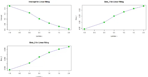
confidence interval. The comparison was made in regard to the other three models (naive model, quadratic model, and the linear model). The results of the various simulations are represented in table 1 below. The study did not show a significant change in the estimates in spite of the increased number of iteration. The SIMEX model using the fitting method as quadratic performed well with all its RMSE being the smallest among all models. In addition, the SIMEX model using quadratic fitting method had the highest coverage rate among the three models. Figure 1 shows the
performance of SIMEX using quadratic as the fitting method. The three graphs demonstrate a consistent trend and extrapolation of the graph to the value of H = −1 gives an approximate of the true coefficients as 4.7661, 40.4160, _(` + 40.0984 which are approximate to
5, 40.5 _(` + 40.1 . The naive model
performed poorest since it was the model that we initially introduce the measurement error.
Figure 1. Plots for the estimates of the SIMEX model using the quadratic fitting method.
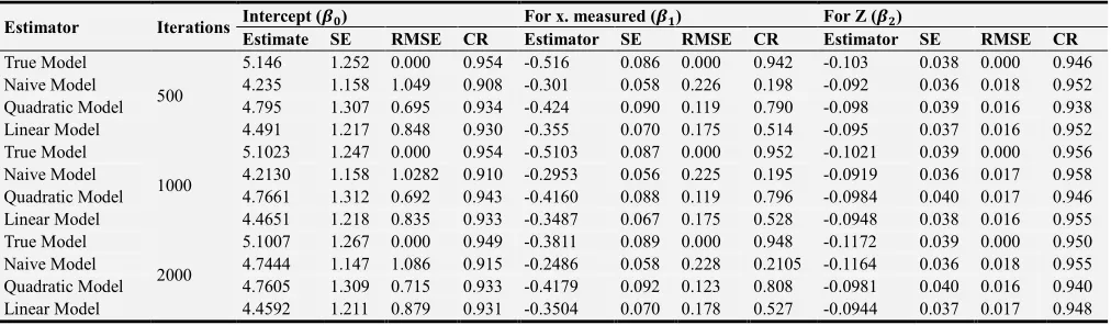
Table 1. The results for model estimates, Standard Error, Root Mean Square Error and Coverage Rate for the different models.
Estimator Iterations Intercept (fg) For x. measured (fh) For Z (fi)
Estimate SE RMSE CR Estimator SE RMSE CR Estimator SE RMSE CR
True Model
500
5.146 1.252 0.000 0.954 -0.516 0.086 0.000 0.942 -0.103 0.038 0.000 0.946
Naive Model 4.235 1.158 1.049 0.908 -0.301 0.058 0.226 0.198 -0.092 0.036 0.018 0.952
Quadratic Model 4.795 1.307 0.695 0.934 -0.424 0.090 0.119 0.790 -0.098 0.039 0.016 0.938
Linear Model 4.491 1.217 0.848 0.930 -0.355 0.070 0.175 0.514 -0.095 0.037 0.016 0.952
True Model
1000
5.1023 1.247 0.000 0.954 -0.5103 0.087 0.000 0.952 -0.1021 0.039 0.000 0.956
Naive Model 4.2130 1.158 1.0282 0.910 -0.2953 0.056 0.225 0.195 -0.0919 0.036 0.017 0.958
Quadratic Model 4.7661 1.312 0.692 0.943 -0.4160 0.088 0.119 0.796 -0.0984 0.040 0.017 0.946
Linear Model 4.4651 1.218 0.835 0.933 -0.3487 0.067 0.175 0.528 -0.0948 0.038 0.016 0.955
True Model
2000
5.1007 1.267 0.000 0.949 -0.3811 0.089 0.000 0.948 -0.1172 0.039 0.000 0.950
Naive Model 4.7444 1.147 1.086 0.915 -0.2486 0.058 0.228 0.2105 -0.1164 0.036 0.018 0.955
Quadratic Model 4.7605 1.309 0.715 0.933 -0.4179 0.092 0.123 0.808 -0.0981 0.040 0.016 0.940
Linear Model 4.4592 1.211 0.879 0.931 -0.3504 0.070 0.178 0.527 -0.0944 0.037 0.017 0.948
SE = Standard Error.
RMSE = Root Mean Square Error.
CR = Coverage Rate based on Standard Error (SE).
4. Conclusion and Recommendation
The study confirmed that the SIMEX method is ideal in correcting errors for the covariates measured with errors. For the two SIMEX fitting methods that were considered, the quadratic fitting method proved to be the best having the smallest RMSE among the models considered and having the highest coverage probability. The high coverage probability means that many of the predicted values will fall within the 95% confidence interval. Consequently, the study proved the power of simulation extrapolation as a method of error corrections. Hence for independent variables which are collected with measurement errors, the researcher should consider the SIMEX method with the fitting method as quadratic to correct the errors and have the correct estimates of the model’s coefficients that will give better approximations of the response variable.
The study recommends the use of the SIMEX method with the fitting method as the quadratic for correcting covariates with errors. Further studies can be done using other statistical models to reaffirm the claims from this study.
References
[1] Fuller, Wayne A. Measurement error models. Vol. 305. John Wiley & Sons, 2009.
[2] Cook, John R., and Leonard A. Stefanski. "Simulation-extrapolation estimation in parametric measurement error models." Journal of the American Statistical association 89, no. 428 (1994): 1314-1328.
[3] Freedman, Laurence S., Douglas Midthune, Raymond J. Carroll, and Victor Kipnis. "A comparison of regression calibration, moment reconstruction and imputation for adjusting for covariate measurement error in regression." Statistics in medicine 27, no. 25 (2008): 5195-5216.
[4] Stefanski, Leonard A., and James R. Cook. "Simulation-extrapolation: the measurement error jackknife." Journal of the American Statistical Association 90, no. 432 (1995): 1247-1256.
[5] Babanezhad, Manoochehr. "Measurement error and causal inference with instrumental variables." PhD diss., Ghent University, 2009.
[6] Rudemo, Mats, David Ruppert, and J. C. Streibig. "Random-effect models in nonlinear regression with applications to bioassay." Biometrics (1989): 349-362.
[7] Stefanski, Leonard A. "Measurement error models." Journal of the American Statistical Association 95, no. 452 (2000): 1353-1358.
[8] Carroll, Raymond J., and Helmut Küchenhoff. "Approximative Methods for Regression Models with Errors in the Covariates." In XploRe: An Interactive Statistical Computing Environment, pp. 275-285. Springer, New York, NY, 1995.
[9] Shang, Yi. "Measurement error adjustment using the SIMEX method: An application to student growth percentiles." Journal of Educational Measurement 49, no. 4 (2012): 446-465. [10] Weeding, Jennifer Lee. "Bayesian measurement error
modeling with application to the area under the curve summary measure." PhD diss., Montana State University-Bozeman, College of Letters & Science, 2016.
[11] Küchenhoff, Helmut, Samuel M. Mwalili, and Emmanuel Lesaffre. "A general method for dealing with misclassification in regression: The misclassification SIMEX." Biometrics 62, no. 1 (2006): 85-96.
[12] Mwalili, Samuel Musili. "Bayesian and frequentist approaches to correct for misclassification error with applications to caries research." PhD diss., PhD thesis, Catholic University of Leuven, Leuven, Belgium, 2006.
[13] Hasan, Mohammad Mahadi, Ashish Sharma, Fiona Johnson, Gregoire Mariethoz, and Alan Seed. "Correcting bias in radar Z–R relationships due to uncertainty in point rain gauge networks." Journal of hydrology 519 (2014): 1668-1676. [14] Tsamardinos, Ioannis, Amin Rakhshani, and Vincenzo Lagani.
"Performance-estimation properties of cross-validation-based protocols with simultaneous hyper-parameter optimization." International Journal on Artificial Intelligence Tools 24, no. 05 (2015): 1540023.