Simulating the Differential Positioning Mode Using One GPS Receiver

(1)

doi: 10.11648/j.jccee.20170202.15

Simulating the Differential Positioning Mode Using One

GPS Receiver

Ahmed Abobakr Elashiry, Abdel Hameid M. Abdel Hameid

Faculty of Engineering, Beni-Suef University, Beni-Suef, Egypt

Email address:

eng_ahmedashiry@yahoo.com (A. A. Elashiry), amonged@yahoo.com (A. H. M. A. Hameid)

To cite this article:

Ahmed Abobakr Elashiry, Abdel Hameid M. Abdel Hameid. Simulating the Differential Positioning Mode Using One GPS Receiver. Journal of Civil, Construction and Environmental Engineering. Vol. 2, No. 2, 2017, pp. 78-86. doi: 10.11648/j.jccee.20170202.15

Received: March 10, 2017; Accepted: March 21, 2017; Published: April 14, 2017

Abstract:

This research tends to raise the accuracy of absolute point positioning by simulating the differential positioning mode. This process was done by observing the unknown point using one unit GPS receiver after observing the fixed point with the same receiver and estimate the Doppler value; where it equals to the expected change at carrier phase measurement from two adjacent epochs, to determine the phase value in the following epoch and generate new observation file for the known point has phase observation at the same period of observing the unknown point. The generated data at the known point will be solved with the observed phase data at the unknown point for four satellites at least using triple difference technique to vanish the ambiguity value and all affecting errors on observations. Finally the least square technique will be applying on the resulted equations from the previous process. This method had been enhanced to improve the positioning accuracy from ten meters to 30 cm as a maximum error in 3D coordinates. In condition that there is one fixed point at least in the observation area, and the interval period between observing the fixed and unknown point is less than 15 min.

Keywords:

GPS, Absolute Point Positioning, Phase Measurements, Doppler Estimations

1. Introduction

With GPS one can automatically determine the location (latitude, longitude and Altitude) at any point on the earth surface and at any time. GPS has many useful applications in many fields such as Surveying (control point), Mapping,

Agriculture, Aviation, Marine Geodesy, Military, GIS, Scientific Studies related to the ionosphere and troposphere, glaciology... etc.

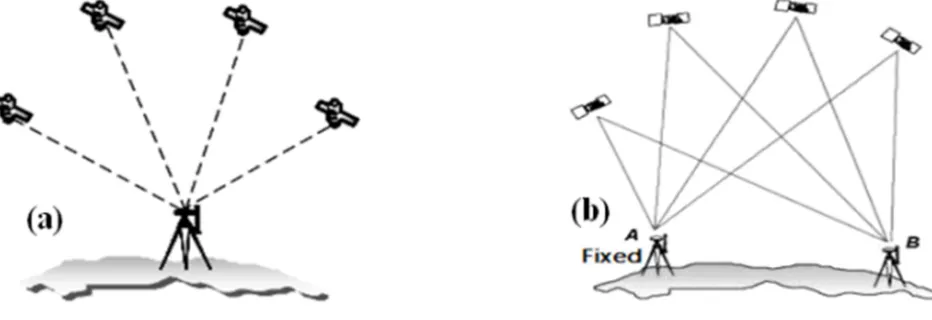
Positioning using GPS can be achieved either through Absolute Point Positioning technique (APP) or through Differential Global Positioning technique (DGPS) (Figure 1).

(2)

In the Differential GPS Positioning (DGPS), two or more receivers are used, where one is setup at a known point (Base), and the other are moved (Rovers) on the unknown points [1]. But the Absolute Point Positioning (APP) uses one unit receiver which occupies an unknown point to determine its position.

There are several sources of errors that degrade the GPS positioning from few meters to tens of meters. These sources of errors are orbital errors: ionospheric and tropospheric delays, satellite and receiver clock errors, multipath, biases, and cycle slip [2]. These errors have more effects on accuracy of the absolute point positioning technique. However, in the DGPS technique, the positioning coordinates of the unknown points are determined relative to the positioning coordinates of the base station (known point). Therefore, most of these errors can be reduced or eliminated through the differences processes. By this method, the accuracy can reach to sub-centimeters for the baseline less than 20 km [3].

The Absolute Point Positioning technique (APP) has two levels from positioning service according to the accuracy, which are Standard Point Positioning (SPP) and Precise Point Positioning (PPP) [4]. The first technique, SPP uses the broadcast ephemeris data in estimating the receiver position [5], where its accuracy is about ten meters [6 and 7]. The second technique, PPP uses the observations of International GPS Service (IGS), precise GPS orbit and clock products supplied by IGS also. The PPP has been widely demonstrated that it is capable of providing positioning accuracy reaches one meter level; if the range is free from ionospheric delay [8].

Basically, there are two kinds of measurements which can be used for determining the GPS positioning: pseudo-code and phase measurements. Both measurements are subjected to the above mentioned affecting errors on the observations

[9]. The results of the phase measurements are more accurate than that of the code measurement [10], because the code measurements suffer from great bias.

On almost precise surveying using GPS the applied technique is the DGPS; where it is the most accurate technique, but it is costly because it requires more than one GPS receiver and more than one employee. On the other hand the Absolute Point Positioning technique is more economic and easier than the DGPS technique because it requires one GPS receiver and one employee, but its accuracy is low. So the problem is the accuracy improvement of the Absolute Point Positioning technique. Thus the aim of this research is to raise the accuracy of APP through development of the new observation method was done by A. A. Elashiry at 2015 [11 and 12] using one GPS receiver to simulate the differential GPS positioning mode by generate phase observations at the known point using Doppler estimations.

2. Proposing Procedure

The proposing procedure consists of two main parts which are: 1- doing and collecting some field observations data 2- using this data in establishing and testing a new method for enhancing the absolute point positioning.

2.1. Field Observations

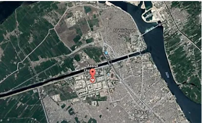
The field work was collected from a studied area in the Assiut University campus, Assiut, Egypt (Figure 2). There is one fixed point called M, has been fixed by the Egyptian Surveying Authority; where its coordinates are shown in (Table 1).

(3)

Table 1. The coordinates of fixed point (M).

Old Egypt 1906 datum (E, N and h)

642190.7 509720.120 115.612

Geodetic datum (WGS84) (Lat, Long and h)

27° 17' 25.06754" N 31° 16' 34.40477" E 115.612 ECEF datum (X, Y and Z)

4847990.25 2944869.44 2906897.9

All studied points observed by two GPS receivers (Z_Xtreme, Ashtech-Magellan, USA) of baseline accuracy

±(5mm + 1ppm) for horizontal and ±(10mm + 1ppm) for vertical through static observation technique; it includes also, antennas, tools and devices such as tripods, tribrachs, cables, batteries and tapes. Each receiver has 12 channels and full wavelength carried on L1 and L2 (Figure 3).

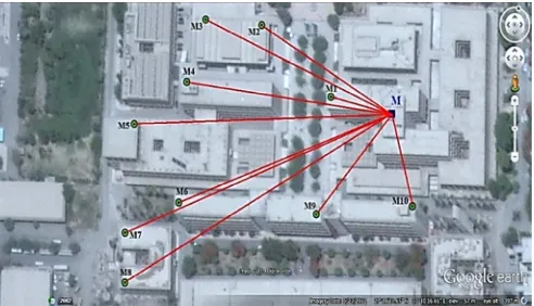
In the studied area some points had been observed to establish this study, named M1, M2, M3, M4, M5, M6, M7, M8, M9 and M10 as shown in (Figure 4).

Figure 3. The used GPS receiver and related Equipment.

(4)

The precise coordinates of all studied points had been determined by using the differential technique (Table 2); where these coordinates were used as reference. The observation parameters were: mask angle = 12, epoch interval= 1 sec and the occupation period = 20 min.

Table 2. The precise coordinates of all tested points in the studied area (using DGPS technique) in Old Egypt datum.

Studied area Point ID East (m) North (m) h (m)

Campus of the Assiut University (FIXED POINT M)

M1 631846.7 498204.9 70.484

M2 631785.9 498233.9 62.616

M3 631738.3 498222.4 62.548

M4 631739.8 498180.1 70.444

M5 631715.7 498146.7 70.328

Studied area Point ID East (m) North (m) h (m)

M6 631759.9 498100.4 71.248

M7 631718.7 498082 60.907

M8 631728.4 498049.2 60.973

M9 631864.1 498120.9 72.798

M10 631927.1 498148.9 71.257

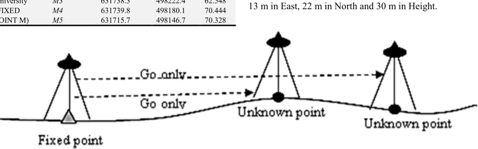
All the studied points were observed using one unit receiver after observing the fixed point with the same receiver at varies interval times 5, 10, 15, 20, 25 and 30 minutes (Figure 5). The average errors in coordinates at case of observing the studied points with one GPS receiver were 13 m in East, 22 m in North and 30 m in Height.

Figure 5. The usage positioning method, (Elashiry observation method).

The downloaded data files from the receiver unit for each observed point are called Receiver INdependent EXchange (RINEX) files version 2.0, and divided into three types 1- observation file, 2- navigation file and 3- meteorological file. The observation data at observation RINEX 2.0 file for any observed satellite at each observation epoch are: phase measurements (L1 phase and L2 phase), code pseudorange (C code, P1 code and P2 code) and Doppler shift (D1 and D2).

2.2. Generating the Virtual Phase Observation

The Doppler value (Di) equals to the expected change at carrier phase measurement from two adjacent epochs [13]. So, this solving technique is based on establishing virtual phase measurements in the RINEX observation file of the known point at all observation periods for unknown point by using Doppler estimation. There are six major steps are as follow:

Firstly use Elashiry detecting model for cycle slip error [14] (from Eq. 1 to Eq. 6) in the phase observations at each observation epoch in the known point and the unknown point RINEX observation files to delete the infected epochs with this error.

L v AX (1)

where, X = Matrix of the unknowns, A = Matrix of coefficients, and L = Matrix of the observations. After subtracting each observable equation at a certain epoch from the adjacent epoch, the final forms of all observables equations, according to the form of basic equation of the Least Square technique (Eq. 1), are as follows: ∆ v ∆ ∆I (2)

∆ v ∆ ∆I (3)

ΔP v Δ ∆I Δbias (4)

ΔP v Δ ∆I Δbias (5)

The related least squares normal equation is as follows [15]: X A A A L (6)

where, the matrices of these equation terms can be detailed as follows: X ! " " # ∆∆I Δbias Δbias $% % & L ! " " " #∆_∆ ΔP ΔP $% % % & ' ! " " " " # 1 1 0 0 1 0 0 1 1 1 0 1 _{0 1 $}%% % % & Secondly use the precise ephemeris data to estimate the precise GPS satellite coordinates and its velocity at any epoch as follow [16 and 17]: The time from reference epoch (+_,): +, -+. +/0 (7)

(5)

Ephemeris reference time, sec.

+,

1 23344, 9:< 6 66=3 56 766,9:34; 6 66 4= 6 66

34<56 766 0>?0@A0.0

Computed mean motion (B_/):

B/ C_EDF (8)

Where, µ is Earth gravitational constant = 3.986004418*1e14 m3/sec2.

Corrected mean motion (B :

B B/ ∆B (9)

Mean anomaly G_, :

G, G/ B+, (10)

Eccentric anomaly (Kepler’s equation) (E_I):

EI MI e SinEI (Solved by iteration) (11) True anomaly (N_,):

+OBN, √1 Q R_V/?US9TU₄4₀ (12)

Argument of latitude (in the orbital plane) _, :

, N, W (13)

Argument of latitude correction XY_, :

XY, C[\ Sin 2 , C[^ Cos 2 , (14) Radius correction X`_, :

X`, Ca\ Sin 2 , Ca^ Cos 2 , (15)

Inclination correction (Xb_, :

Xb, Cc\ Sin 2 , Cc^ Cos 2 , (16)

Corrected argument of latitude (Y_,):

Y, , XY, (17) Corrected radius (`_,):

`, O 1 Qdefg, X`, (18) Corrected inclination (b_,):

b, b/ Xb, +,bh/3 (19) Position x in the orbital plane (ij_,):

ij, `,defY, (20)

Position y in the orbital plane (kl_,):

kl, `,mbBY, (21)

Corrected longitude of ascending node (n_o):

no n/ +,R pnq– nq0s +/0R nQ (22)

nq0: WGS earth rotation parameter = 7.2921151467*1e-5 rad/sec.

Earth-Centered, Earth-Fixed Coordinates (ECEF)

t, ij,defΩ, kl,defi,mbBΩ, (23)

v, ij,mbBΩ, kl,defi,defΩ, (24)

w, kl,mbBi, (25) Satellite velocity:

tq, ij,q defΩ, kl,q defi,mbBΩ, kl,mbBi,mbBΩ,ıq,q y,Ω,q (26)

vq, ij,q mbBΩ, kl,q defi,defΩ, kl,defi,ıq,q defΩ, x,Ω,q (27)

wq, kl,q mbBi, kl,defi,ıq,q (28)

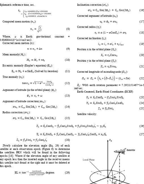
Thirdly calculate the elevation angle (Eq. 29) of each satellite at each observation epoch (Figure 6) to determine the satellites PRN which will be found in the following epochs [18]. Where if the elevation angle of any satellite at any epoch less than the inserted angle in the receiver means this satellite isn't found at the sight and it must be deleted at this epoch.

EL +OB {0.39|E>

}0E?3 <T/.3A , degrees (29)

(6)

where,

Be`+~ •ef €. • fbB ‚. • ƒi fbB €. • fbB ‚.

• ƒk •ef ‚. • ƒ„

QOf+ fbB €. • ƒi •ef €. • ƒk

NQ`+b•O… •ef €. • •ef ‚. • ƒi fbB €.

• •ef ‚. • ƒk fbB ‚. • ƒ„

where,

ƒi ?E3† /‡?†_. ; ƒk ?E3‰ /‡?‰_. ; ƒ„ ?E3Š /‡?Š_. ; satX,

satY and satZ are the satellite coordinates, m; obsX, obsY and obsZ are the receiver coordinates, m; r is the unit vector from observation station to satellite position, and €_.,‚_. are the receiver latitude and longitude.

Fourthly use the precise ephemeris data to estimate the Doppler value (Eq. 30) [27] starting from the following epoch (i+1) for the last good epoch (i) at the known observation point and then calculate the virtual phase at the new epoch (i+1) (Eq. 31).

‹9 @Œ @_| ••_•.._ŒŒ ._.•_•_• •9 (30)

where, Di is the Doppler value; wi is the satellite velocity; wu is the receiver velocity; c is the speed of light; ri is the satellite location; ru is the receiver location, and L1 is the frequency transmitted by the satellite.

Phase i+1 = phase i +Di (31)

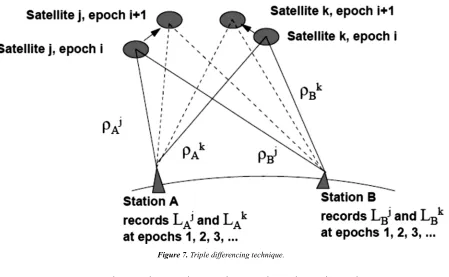
Fifthly after generating the new RINEX file, which has the virtual observation for a known point, this observation can be solved differentially with the observations of the unknown point using triple differencing technique (Eq. 32). Where in triple differencing (Figure 7), consider two successive epochs (i, i+1) of double differenced data from receivers A and B observing satellites j and k, which means that two receivers observe two satellites at two epochs [20]. The big advantage of this differencing is that the ambiguity term is cancelled; and therefore, it is immune to changes in ambiguity.

Figure 7. Triple differencing technique.

λ c _c’“”• c–“”• c’—”• c–—”• c’“” c–“” c’—” c–—”

ρ’“”• ρ–“”• ρ’—

”• ρ–—

”•

ρ’“” ρ–“” ρ’—

” ρ–—

”

(32)

where, ϕ is the measured phase obtained from observation RINEX file (cycle); Li is the phase type L1 or L2; and ρ is the true geometric distance between the receiver and the satellite (m)

Sixthly and finally use least square model (Eq. 6) for solving the resulting equations for four satellites at least to

determine the unknown points coordinates

(7)

(8)

3. Results

The results from using Doppler estimation in all studied points to generate virtual data (estimated data) of phase measurements, shown in (Figure 9), refer to that; the

maximum error in 3D positioning coordinates is less than 30 cm at interval time between observing the unknown point after the known point less than 15 minutes.

Figure 9. Errors in 3D Coordinates at all studied points resulting from using the virtual phase at different times between observing the fixed and unknown points.

4. Discussions

The results refer to also inverse relationship between the positioning error and time; that due to the used data in the Doppler equation has a difference from the precise data determined by receiver so the estimated Doppler different from the precise Doppler, where the estimated phase in the present epoch depends on the estimated Doppler in the previous epoch, thus the error will accumulate with time and caused in accumulating the error in positioning coordinates.

5. Conclusion

The usage method in this research had been enhanced to improve the positioning accuracy from 13 m in East, 22 m in North and 30 m in Height as average error to 30 cm as a maximum error in 3D coordinates. In condition that there is one fixed point at least in the observation area, and the interval period between observing the fixed and unknown

point is less than 15 min.

References

[1] EL-Rabbany, A., "Introduction to GPS (The Global Positioning System)", Artech House, 2002.

[2] Petrovskyy, V., et. al., "Precise GPS Position and Attitude", GPS Technology Projects, Aalborg University, 2007.

[3] El-Rabbany," Precise GPS Point Positioning: the Future Alternative to Differential GPS Surveying", Ryerson University, 2002.

[4] Sunehra, D., "Estimation of Prominent Global Positioning System Measurement Errors for GAGAN Applications", European Scientific Journal, Vol. 9, pp 68-81, 2003.

(9)

[6] Alkan, R. M., et. al., "GPS Standard Positioning Service Performance After Selective Availability Turned Off ", International Symposium In GIS, the International Federation of Surveyors (FIG), 2002.

[7] Chen, H. W., et al., “A New Coarse-Time GPS Positioning Algorithm Using Combined Doppler and Code-Phase Measurements”, GPS Solution, Vol. 8, DOI 10.1007/s10291-013-0350-8, 2013.

[8] Chen, K., "Real-Time Precise Point Positioning Using Single Frequency Data" Proceedings of the Institute Of Navigation ION GNSS, 2005.

[9] CHANG, X. W. et. al., “An Algorithm for Combined Code and Carrier Phase Based GPS Positioning”, BIT Numerical Mathematics Vol. 43, pp 915 - 927, 2003

[10] Zeng, F., et. al., ”Single-Point Positioning with the Pseudorange of Single-frequency GPS Considering the Stochastic Model”, Pacific Science Review, Vol. 10, No. 3, pp. 274-278, 2008.

[11] Elashiry, A. A., et. al., “Adjusting of Absolute Point Positioning Accuracy”, 7th International Conference On Emerging Technologies in Civil Engineering, Architecture and Environmental Engineering for Global Sustainability, New Delhi, Indian, Journal of Basic and Applied Engineering Research, Volume 2, Number 8; April-June, 2015.

[12] Elashiry, A. A., et. al., ”Enhancement Of The Single Point Positioning Accuracy (Using The Observations Of IGS Service)”, International Journal of Civil, Structural, Environmental and Infrastructure Engineering Research and Development journal, Vol. 5, Issue 3, Jun 2015.

[13] Silva, P., "Cycle Slip Detection and Correction for Precise Point Positioning", Proceedings of the Institute of Navigation ION GNSS, 2013.

[14] Elashiry, A. A., et. al., “Modification Of Phase-Phase And Phase-Code Methods For Precise Detection And Prediction Of GPS Cycle Slip Error”, International Journal of Unmanned Systems Engineering (IJUSEng),

http://dx.doi.org/10.14323/ijuseng.2015.16, Vol. 3, Issue 4, 2015

[15] Guochang X., "GPS Theory Algorithms and Applications". (2nd ed.). Springer-Verlag. Berlin. Heidelberg, 2007.

[16] Grewal, M. S., "Global Positioning System, Inertial Navigation, and Integration", 2nd Edition, A John Wiley & Sons, Inc, 2007.

[17] ICD, "Navstar GPS Space Segment/ Navigation User Interfaces", Arinc Research Corporation, ICD-GPS-200C, 1993.

[18] Gustavsson, P., "Development of a Matlab Based GPS Constellation Simulation for Navigation Algorithm Developments", Master's Thesis, Space Science Department, Lulea University of Technology, 2005.

[19] Ren, Z., et. al., "Instantaneous Cycle-Slip Detection and Repair of GPS Data Based on Doppler Measurement", International Journal of Information and Electronics Engineering, Vol. 2, No. 2, 2012.