Multirate signal processing concepts in digital communications

(1)

in Digital Communications

Thesis by

Bojan Vrcelj

In Partial Fulﬁllment of the Requirements for the Degree of

Doctor of Philosophy

1 8 9 1

C A L

I

F

O

RN

IA

IN

ST IT

U_{T E O} F T

E C

H

N

O

L

O G

Y

California Institute of Technology Pasadena, California

2003

(2)

c

2003

(3)

Acknowledgments

First of all, I would like to express my profound gratitude to my advisor, Professor P.P. Vaidyanathan, for his outstanding guidance and support during my stay at Caltech. P.P. is a fascinating teacher and a thoughtful mentor, always ready to share his expertise with the students. He is also a thorough, brilliant researcher and I beneﬁted greatly from working under his guidance. His encouragement and friendship have been invaluable throughout my studies at Caltech. His academic excellence continues to be a source of inspiration, but beyond that I am especially grateful for his limitless patience and fatherly support during trying times.

I would like to thank the members of my defense and candidacy examining committees for their interest: Prof.Robert McEliece, Prof.Babak Hassibi, Prof.Emmanuel Candes, Dr.Murat Me¸se, Dr.Dariush Divsalar and Prof.Pietro Perona. I would also like to thank the professors at the school of Electrical Engineering, University of Belgrade, for providing me with solid foundations which have proved helpful throughout my studies. I should single out my diploma thesis adviser, Prof.Miodrag Popović. My thanks also go to my high school physics teacher, Ms.Nataˇsa ˇCaluković, who sparked my interest in the field of electrical engineering.

I would like to thank my present and past lab-mates, Andre Tkacenko, Murat Me¸se, Sony Akkarakaran, Sriram Murali, and Byung-Jun Yoon, who helped create a very enjoyable and productive environment in the DSP lab. Sony and Murat were mid-way through their doctorate studies when I joined the group. I feel indebted to them for their friendship, support, patience and collegial help, which was so essential during my first year at Caltech. Andre has been my office-mate and a good friend for four years now. I deeply value our academic and personal discussions as well as our daily shots of caffeine. Byung-Jun and Sriram joined our lab two years ago and made the atmosphere even more friendly and enjoyable.

I am grateful to many other people, some aﬃliated with Caltech, and the others whom I have known long before I joined, for their friendship, company, and entertainment, that helped make my life outside the oﬃce very pleasant. I also feel that my Caltech experience was greatly enriched by the institute-wide groups, clubs and organized events. In this capacity I would like to thank the people of the Caltech Y, International Student Program and the water polo crowd.

(4)

Abstract

Multirate systems are building blocks commonly used in digital signal processing (DSP). Their function is to alter the rate of the discrete-time signals, which is achieved by adding or deleting a portion of the signal samples. Multirate systems play a central role in many areas of signal processing, such as ﬁlter bank theory and multiresolution theory. They are essential in various standard signal processing techniques such as signal analysis, denoising, compression and so forth. During the last decade, however, they have increasingly found applications in new and emerging areas of signal processing, as well as in several neighboring disciplines such as digital communications.

The main contribution of this thesis is aimed towards better understanding of multirate systems and their use in modern communication systems. To this end, we ﬁrst study a property of linear systems appearing in certain multirate structures. This property is calledbiorthogonal partnershipand represents a terminology introduced recently to address a need for a descriptive term for such class of ﬁlters. In the thesis we especially focus on the extensions of this simple idea to the case of vector signals (MIMO biorthogonal partners) and to accommodate for nonintegral decimation ratios (fractional biorthogonal partners).

Some of the main results developed here pertain to a better understanding of the biorthogonal partner relationship. These include the conditions for the existence of stable and of finite impulse response (FIR) biorthogonal partners. A major result that we establish states that under some generally mild conditions, MIMO and fractional biorthogonal partners exist. Moreover, when they exist, FIR solutions are not unique. We develop the parameterization of FIR solutions, which makes the search for the best partner in a given application analytically tractable. This proves very useful in the central application of biorthogonal partners, namely, channel equalization in digital communications with signal oversampling at the receiver. Sampling the received signal at a rate higher than that defined by the transmitter provides some flexibility in the design of the equalizer. A good channel equalizer in this context is one that helps neutralize the distortion on the signal introduced by the channel propagation but not at the expense of amplifying the channel noise. This presents the rationale behind the partner design problem which is formulated and solved. The performance of such equalizers is then compared to several other equalization methods by computer simulations. These findings point to the conclusion that the communication system performance can be improved at the expense of an increased implementational cost of the receiver.

(5)

avoid severe noise ampliﬁcation at the receiver, and so forth. In the second part of the thesis, we focus on this second group of multirate systems, derive some of their properties and introduce certain improvements of the communication systems in question.

We first consider the transmission systems that introduce the redundancy in the form of a cyclic prefix. The examples of such systems include the discrete multitone (DMT) and the orthogonal frequency division multiplexing (OFDM) systems. The cyclic prefix insertion helps to effectively divide the channel in a certain number of nonoverlaping frequency bands. We study the problem of signal precoding in such systems that serves to adjust the signal properties in order to fully take advantage of the channel and noise properties across different bands. Our ultimate goal is to improve the overall system performance by minimizing the noise power at the receiver. The special case of our general solution corresponds to the white channel noise and the best precoder under these circumstances simply performs the optimal power allocation.

(6)

List of Figures

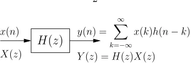
1.1 Filtering operation: linear time invariant system. . . 2

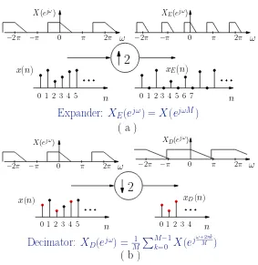
1.2 Multirate building blocks: (a) 2-fold expander and (b) decimator. . . 3

1.3 The deﬁnition and the notation of the vector signal expander. . . 3

1.4 Notations: blocking (a) and unblocking (b) operations. . . 4

1.5 Signal recovery after interpolation: (a) using ﬁlter inverses, and (b) using ‘generalized inverses.’ 5 1.6 Biorthogonal partners: (a) deﬁnition and (b) equivalent LTI system. . . 5

1.7 Nyquist(M) property demonstrated forM = 3. . . 6

1.8 Biorthogonal partners in biorthogonal ﬁlter banks. . . 7

1.9 Block diagram of a general communications system. . . 8

1.10 Polyphase representations of (a) ﬁlter bank precoder and (b) analysis ﬁlter bank. . . 9

1.11 Channel magnitude response divided in frequency bands. . . 10

2.1 Block diagram interpretation of a left biorthogonal partner. . . 16

2.2 Pertaining to the proof of Theorem 2.1. . . 17

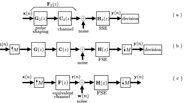
2.3 (a) Discrete-time equivalent of a digital communication system with SSE; the equivalent chan-nel is F₂(z) = C₂(z)G₂(z). (b) Digital communication system from (a), now equalized with FSE H(z). (c) Further simpliﬁcation of the system from (b); the equivalent channel isF(z) =C(z)G(z). . . 23

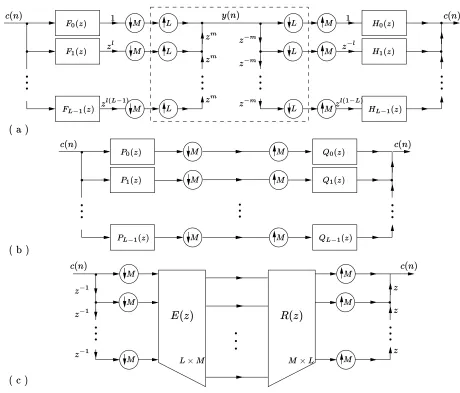
2.4 Block diagram interpretation of the construction of FSE forM = 2. (a) Discrete-time equiv-alent communication channel with FSE, (b) equivequiv-alent of (a) obtained using noble identities [61], and (c) equivalent model for noise. . . 25

2.5 (a)-(b) Equivalent structures for FIR LBPs. . . 26

2.6 (a)-(b) MIMO FSEs and MIMO LBPs. . . 27

2.7 (a)-(b) Finding the optimal FIR LBP. . . 27

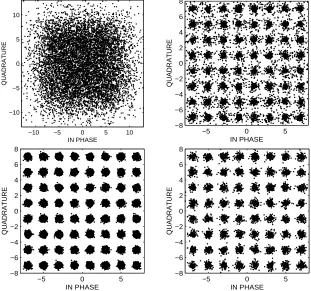
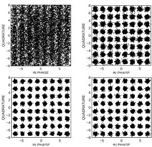
2.8 Equalization results. Clockwise, starting from upper left: SSE, plain FIR FSE, optimized FIR FSE as in Section 2.4.1, and optimized FIR FSE as in Section 2.4.2. . . 29

2.9 Probability of error as a function of the estimator order: (left) square 3×3 channel, and (right) rectangular 2×3 channel—see the text. . . 30

2.10 Least squares signal modeling: (a) signal model and (b) least squares solution (see text). . . . 31

(10)

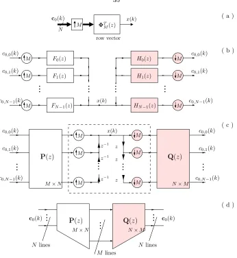
2.12 Prefiltering for multiwavelet transform. (a) Signal model. (b) Equivalent drawing of (a) together with the prefiltering part. (c) Equivalent drawing using polyphase matrices. (d) Final form of the traditional method for prefiltering by left-inverting the polyphase matrix.

See text. . . 35

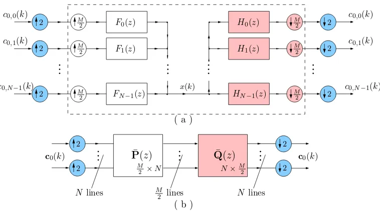
2.13 Biorthogonal partners in preﬁltering for multiwavelet transform. (a) Equivalent of Fig.2.12(b) for evenM. (b) Equivalent of Fig.2.12(d) for evenM. See text. . . 37

3.1 Example of a generating functionφ(t) (cubic spline) and its three times ‘stretched’ versionf(t). 44 3.2 (a) Signal model. (b) Scheme for reconstruction. . . 45

3.3 (a)-(b) Equivalent presentations of fractional biorthogonal partners. . . 46

3.4 (a)-(b) Some multirate identities. . . 47

3.5 (a)-(c) Further simpliﬁcations of fractional biorthogonal partners. . . 48

3.6 Continuous-time communication system. (a) Transmitter and channel. (b) Receiver. . . 49

3.7 FSEs with fractional oversampling. (a) Discrete-time model of the communication system. (b) Form of the proposed equalizer. . . 51

3.8 Communication system with FoFSEs. (a) FBP form. (b) Blocked equivalent form. . . 51

3.9 (a)-(b) Finding the optimal FIR RFBP. See text. . . 52

3.10 Equalization results. Clockwise, starting from upper left: SSE, plain FIR RFBP, optimized FIR RFBP and MMSE methods. . . 54

3.11 Probability of error as a function of SNR in the four equalization methods. . . 55

3.12 Probability of error as a function of noise variance discrepancyα2. . . 55

3.13 Interpolation of discrete signals using digital ﬁltering. In the case of spline interpolation, φ_K(t) is an oversampled B-spline. . . 56

3.14 (a) Signal model and proposed interpolation. (b) Scheme for all-FIR interpolation. . . 57

3.15 FIR interpolation example: a region of the image oversampled byL/M = 6/5 and its cubic spline interpolation by a factor ofM K/L= 5/3 obtained using FIR ﬁlters. . . 58

3.16 Least squares problem. (a) Signal model. (b)-(c) Equivalent drawing. . . 59

3.17 Least squares problem revisited in MIMO biorthogonal partner setting. (a) Signal model. (b) Least squares approximation. . . 60

3.18 (a)-(b) Solution to the least squares problem. . . 60

3.19 (a) Deﬁnition of vector FBPs. (b) Construction of vector FBPs. . . 62

4.1 (a) Input symbol stream, (b)-(c) explanation of how cyclic preﬁx is inserted. . . 66

4.2 Channel with the system for cyclic preﬁx. . . 66

4.3 Cyclic preﬁx system with all processing at the receiver. . . 67

4.4 Conventional cyclic preﬁx system with DFT matrices used for ISI cancellation. . . 67

(11)

4.6 Receiver and the noise model. . . 69 4.7 Convex polytope deﬁned by the doubly stochastic matrixΩ (left), and concave functionf(·)

deﬁned over this polytope (right). . . 71 4.8 Summary of the parameters used: channel impulse response, zero magnitudes, SNR,

proba-bilities of error. . . 72 4.9 Equalization results using a modiﬁed system without (left), and with the optimal precoder/equalizer

(right). . . 73 4.10 Probability of error vs. SNR: without precoder (dashed line) and with precoder (solid line). . 73 4.11 Cyclic preﬁx system with separated ISI cancellation and noise suppression. Second method. . 74 4.12 Channel input power constraint. . . 74 4.13 Summary of the parameters used: channel zero plot, M, improvement factor. . . 75 4.14 Equalization results using the channel inverse (left), and an optimal precoder/equalizer (right). 76 4.15 Probability of error vs. SNR using the two methods. . . 76

5.1 Discrete-time equivalent of a baseband AMOUR system. . . 80 5.2 (a)-(c) Equivalent drawings of a symbol spaced AMOUR system. . . 82 5.3 (a) Continuous-time model for an AMOUR system with integral oversampling. (b)

Discrete-time equivalent drawing. (c) Polyphase representation forq= 2. . . 85 5.4 Proposed form of the equalizer with rate reduction. . . 87 5.5 (a) A possible overall structure for the FSAMOUR system. (b) Simpliﬁed equivalent structure

for ISI suppression. . . 88 5.6 (a) Equivalent FSAMOUR system. (b) ZFE structure with noise input. . . 90 5.7 Probability of error as a function of SNR in AMOUR and FSAMOUR systems. . . 92 5.8 (a) Continuous-time model for an AMOUR system with fractional oversampling ratioq/r. (b)

Discrete-time equivalent drawing. . . 93 5.9 (a) Discrete-time model for the FSAMOUR system with the oversampling ratio q/r. (b)

Equivalent drawing. (c) Redrawing a block from (b). . . 94 5.10 Proposed structure of the FSAMOUR receiver in systems with fractional oversampling . . . . 100 5.11 Probability of error as a function of SNR in AMOUR and FSAMOUR systems with

(12)

(13)

Chapter 1 Introduction

The theory of multirate digital signal processing (DSP) has traditionally been applied to the contexts of filter banks [61], [13], [50] and wavelets [31], [72]. These play a very important role in signal decomposition, analysis, modeling and reconstruction. Many areas of signal processing would be hard to envision without the use of digital filter banks. This is especially true for audio, video and image compression, digital audio processing, signal denoising, adaptive and statistical signal processing. However, multirate DSP has recently found increasing application in digital communications as well. Multirate building blocks are the crucial ingredient in many modern communication systems, for example, the discrete multitone (DMT), digital subscriber line (DSL) and the orthogonal frequency division multiplexing (OFDM) systems as well as general filter bank precoders, just to name a few. The interested reader is referred to numerous references on these subjects, such as [7]–[9], [17]–[18], [27], [30], [49], [64], [89], etc.

This thesis presents a contribution to further understanding of multirate systems and their signiﬁcance in digital communications. To that end, we introduce some new signal processing concepts and investigate their properties. We also consider some important problems in communications especially those that can be formulated using the multirate methodology. In this introductory chapter, we give a brief overview of the multirate systems and introduce some identities, notations and terminology that will prove useful in the rest of the thesis. Every attempt is made to make the present text as self-contained as possible and the introduction is meant to primarily serve this purpose. While some parts of the thesis, especially those that cover the theory of biorthogonal partners and their extensions provide a rather extensive treatment of the concepts, the material regarding the applications of the multirate theory in communication systems should be viewed as a contribution to a better understanding and by no means the exhaustive treatment of such systems. For a more comprehensive coverage the reader is referred to a range of extensive texts on the subject, for example, [71], [18], [19], [39], [38], [53], etc.

1.1 Multirate systems

1.1.1 Basic building blocks

(14)

Y(z) =H(z)X(z) x(n)

X(z)

H

(

z

)

y(n) =

∞

k=−∞

x(k)h(n−k)

Figure 1.1: Filtering operation: linear time invariant system.

number. Signal processing analysis is often simpliﬁed by considering the frequency domain representation of signals and systems. Commonly used alternative representations of x(n) are its z-transform X(z) and the discrete-time Fourier transform X(ejω). The z-transform is deﬁned as X(z) = ∞_n₌_−∞x(n)z−n, and X(ejω) is nothing butX(z) evaluated on the unit circlez=ejω.

Multirate DSP systems are usually composed of three basic building blocks, operating on a discrete-time signal x(n). Those are the linear time invariant (LTI) ﬁlter, the decimator and the expander. An LTI ﬁlter, like the one shown in Fig.1.1, is characterized by its impulse response h(n), or equivalently by its z-transform (also called the transfer function)H(z). Examples of the M-fold decimator and expander for M = 2 are shown in Fig.1.2. The rate of the signal at the output of an expander isM times higher than the rate at its input, while the converse is true for decimators. That is why the systems containing expanders and decimators are called ‘multirate’ systems. Fig.1.2 demonstrates the behavior of the decimator and the expander in both the time and the frequency domains. In thez-domain this is described by

X_E(z) = [X(z)]_↑_M = X(zM) forM-fold expander, and (1.1)

X_D(z) = [X(z)]_↓_M = 1 M

M−1

k=0

X(zM1 _e−j2Mπk₎ _for_M_{-fold decimator.} _(1.2)

The systems shown in Figs.1.1 and 1.2 operate on scalar signals and thus are called single input— single output (SISO) systems. The extensions to the case of vector signals are rather straightforward: the decimation and the expansion are performed on each element separately. The corresponding vector sequence decimators/expanders are denoted within square boxes in block diagrams. In Fig.1.3 this is demonstrated for vector expanders. The LTI systems operating on vector signals are called multiple input—multiple output (MIMO) systems and they are characterized by a (possibly rectangular) matrix transfer functionH(z).

1.1.2 Some multirate deﬁnitions and identities

(15)

n xE(n)

0 1 2 3 4 6 7

0 π 2π _ω

−π XE(ejω₎

5

2

−2π

0 π 2π

−2π −π X(ejω₎

ω

x(n)

n

0 12 3 4 5

Expander:

X

E

(

e

jω

) =

X

(

e

jωM

)

( a )

2

x(n)

n

0 12 3 4 5 0 1 2 3 4

xD(n)

n

0 π 2π

−2π −π X(ejω₎

ω −2π −π 0 π 2π

XD(ejω)

ω

Decimator:

X

D

(

e

jω

) =

_M1

M_k=0−1

X

(

e

j

ω+2πk

M

)

( b )

Figure 1.2: Multirate building blocks: (a) 2-fold expander and (b) decimator.

M

M M

M

Figure 1.3: The deﬁnition and the notation of the vector signal expander.

of the unblocking and blocking operations is employed.

A very useful tool in multirate signal processing is the so-calledpolyphase representation of signals and systems. It facilitates considerable simplifications of theoretical results as well as efficient implementation of multirate systems. Since polyphase representation will play an important role in the rest of the thesis, here we take a moment to formally define it. Consider an LTI system with a transfer function H(z) =

_∞

n=−∞h(n)z−n and suppose we are given an integer M. We can decomposeH(z) as

H(z) = M−1

m=0

z−m ∞

n=−∞

h(nM +m)z−nM= M−1

m=0

z−mH_m(zM) (Type 1 decomposition). (1.3)

(16)

B

blocking

K K

U

unblocking

K

K K

s(n) s(n)

K

K K

z−1 z−1

z−1

s(n) _s₍_n₎

( b )

s(n)

z

z z

s(n)

( a )

s(n) s(n)

Figure 1.4: Notations: blocking (a) and unblocking (b) operations.

h_m(n), obtained from h(n) by M-fold decimation starting from sample m. In other words, h(n) can be obtained by combining sequencesh_m(n) through the unblocking structure shown in Fig.1.4(b). Subsequences h_m(n) and the correspondingz-transforms deﬁned in (1.3) are called the Type 1 polyphase components of H(z) with respect toM. A variation of (1.3) is obtained if we decimateh(n) starting from sample−m, for 0≤m≤M −1. This gives rise to Type 2 polyphase components ¯H_m(z):

H(z) = M−1

m=0

zmH¯_m(zM) (Type 2 decomposition). (1.4)

The polyphase notation will be used again very soon in Section 1.3.2 when we discuss the use of ﬁlter bank precoders in modern digital communications. However, it is also an important tool in the rest of the thesis. The reader will therefore often be referred to the results from this section. In the following we ﬁrst describe the notion that plays the central role in Chapters 2 and 3, namely, the concept ofbiorthogonal partners.

1.2 Biorthogonal partners

1.2.1 Generalized inverse

(17)

M

x

(

n

)

y

(

n

)

x

(

n

)

M

H

(

z

)

INVERSE

1 /H

(

z

)

( a )

M

x

(

n

)

y

(

n

)

x

(

n

)

M

H

(

z

)

F

(

z

)

( b )

PARTNER BIORTHOGONAL

Figure 1.5: Signal recovery after interpolation: (a) using ﬁlter inverses, and (b) using ‘generalized inverses.’

( a )

( b )

M

F

(

z

)

H

(

z

)

M

G

0

(

z

)

ˆ

x(n)

x(n) xˆ(n)

Figure 1.6: Biorthogonal partners: (a) deﬁnition and (b) equivalent LTI system.

reconstruction scheme. Filters F(z) with the described property are called biorthogonal partners of H(z) and were ﬁrst introduced in [65]. Notice that the inverse ﬁlter is a valid biorthogonal partner. Therefore biorthogonal partners can be thought of as generalized inverses.

Before we provide the formal definition of biorthogonal partners let us answer a potential question: why would we even bother to use the more general reconstruction structure from Fig.1.5(b) if the one in Fig.1.5(a) already works fine? In most practical applications where the interpolation structure arises (e.g.,[59], [74], [65]) filterH(z) has finite impulse response (FIR). Therefore the solution in Fig.1.5(a) involves IIR (infinite impulse response) filtering which is often times unstable or noncausal. In contrast to this, biorthogonal partners often display many desirable properties. Under some mild conditions onH(z) and M there exist stableand evenFIRbiorthogonal partners [65]. Moreover, whenever FIR solutions exist they are not unique. This property will be of special importance in the study of multiple input—multiple output (MIMO) and fractional biorthogonal partners in Chapters 2 and 3, respectively, where we use this non-uniqueness to find the optimal biorthogonal partner for the application at hand.

1.2.2 Deﬁnition and relation to ﬁlter banks

(18)

n

3 6

0

−3

−6

Figure 1.7: Nyquist(M) property demonstrated forM = 3.

in other words if the system in the ﬁgure is the identity. It is a simple exercise to show that the system in question is indeed an LTI system. If we denote the product F(z)·H(z) = G(z), then system from Fig.1.6(a) is equivalent to the one in Fig.1.6(b), where G₀(z) denotes the zeroth polyphase component of G(z) with respect toM. Therefore,F(z) andH(z) are said to form abiorthogonal pair(biorthogonal partner relationship is symmetric) with respect toM if

G₀(z) = [F(z)H(z)]_↓_M = 1. (1.5)

In the time domain (1.5) implies thatg(n), the impulse response ofG(z), satisﬁes the Nyquist(M) condition demonstrated in Fig.1.7. In other words, the sequenceg(n) has zero-crossings at all multiples ofM except whenn= 0. Notice that ifM is changed the two ﬁlters might not remain partners; however, the term ‘with respect toM’ is usually omitted whenever no confusion is anticipated.

As mentioned previously, the phrase ‘biorthogonal partners’ was first introduced in [65]. In the following we motivate this terminology. Consider the perfect reconstruction (PR) orbiorthogonalfilter bank [61] shown in Fig.1.8. Such system is by definition the identity, i.e.,for any input x(n), the output isx(n). Each pair of filters {H_k(z), F_k(z)} in such filter bank forms a biorthogonal pair according to the definition (1.5). To see this, append the analysis bank at the output of the PR filter bank as shown in Fig.1.8. The outputs are obviously given by the sameui(n) that appear in the subbands of the PR filter bank. This is true for any x(n) and thus for any choice ofui(n). Without loss of generality, let us concentrate on the first channel (see the figure). We observe that the marked system betweenu₁(n) andu₁(n) is identical to the one in Fig.1.6(a) and is nothing but the identity system. Therefore H₁(z) and F₁(z) are indeed biorthogonal partners with respect toM.

(19)

M

F₀(z)

FM−1(z)

F₁(z) x(n)

M H₀(z)

HM−1(z)

H₁(z)

u0(n)

u1(n)

M H₀(z)

HM−1(z)

H₁(z)

uM−1(n)

u0(n)

u1(n)

uM−1(n)

BIORTHOGONAL FILTER BANK

x(n)

M

M M

M

Figure 1.8: Biorthogonal partners in biorthogonal ﬁlter banks.

modern communication systems.

1.3 Multirate applications in digital communications

1.3.1 System for digital communication

The block diagram of the communication system that is the focus of this thesis is shown in Fig.1.9. Even though the figure title reads ‘general,’ numerous variations and extensions are possible [39]. The system focuses on a single user with the corresponding discrete messages(n). This message is to be transmitted to the single receiver, only after sustaining the perturbations introduced by the transmission medium. These perturbations are modeled by the continuous-time LTI channel c_c(t) and the appropriate additive noise at the input of the receiver. The design challenge amounts to ensuring that the received sequence s(n) resembles the original message under some criteria (usually in the₂sense). To this end, the receiver often introduces some redundancy combined with the appropriate pre-processing. The goal of this block is to facilitate the signal reconstruction at the transmitter (more about this in the following subsection). The obtained signalx(n) with rate 1/T is converted to analog and sent through the medium to the receiver, only after the pulse-shaping. The combined effect of the pulse-shaping and the physical channel is often referred to as theequivalent channeland denoted byfc(t). At the receiver, the corrupted signal is first sampled and digitized, according to the sampling rateq/T. In this thesis we mostly focus on the case whenq >1 which corresponds to acquiring ‘more information than absolutely necessary’ about the signal and the channel. This further facilitates the signal recovery. The corresponding digital equalizer works at the higher rate and that combined with its increased complexity is the price to pay for the improvement in performance achieved by oversampling. Finally, the signal rate needs to be reduced back to the rate of s(n). This is usually achieved after decimating byqand removing the redundancy.

(20)

0 T 0 T

channel

fc(t)

ﬁlter

g_c(t) c_c(t)

D / A

noise

A / D

y(n)

sample

q/T _EQUALIZER

r_c(t)

pulse-shaping

x(n)

q

s(n)

pre-proc.+

redundancy H(z)

ˆ

s(n)

1/T

redund. removal

Figure 1.9: Block diagram of a general communications system.

In this thesis we mainly focus on the blocks for redundancy insertion and pre-processing together with the corresponding equalization and redundancy removal (Chapter 4), as well as equalization for different values of the parameterqin the vector and the scalar case (Chapters 2, 3). Also, of special interest will be the system modifications for application in multiuser communications and the corresponding equalization algorithms (Chapter 5). Biorthogonal partners play a special role in the equalizer design wheneverq >1, and this is investigated in Chapters 2 and 3. As for the material in the remainder of the thesis, it involves the use of more general multirate structures sometimes called filter bank precoders. In the following subsection we provide the corresponding notation and the equivalent representation.

1.3.2 Multirate systems in digital communications: ﬁlter bank precoders

As noted in Section 1.1.2, the polyphase representation of digital filters is put to use quite often in multirate DSP. One example is in deriving the equivalence between a bank of filters and the correspondingpolyphase matrix. Consider the systems on the left-hand side of Fig.1.10. IfP =K=J, the concatenation of systems in Fig.1.10(b) and Fig.1.10(a) is better known as aP-channel maximally decimated filter bank [61]. However, in most applications in communications P is assumed to be greater than K andJ, therefore the structure is sometimes referred to as an overdecimated filter bank. Consider the structure in Fig.1.10(a). It is better known as the filter bank precoder. Note that the rate ofx(n) is greater than the combined rates of the signals in the vectors(n), therefore the structure is often used to introduce redundancy in the data stream at the transmitter side of a communication system. As mentioned in Section 1.3.1, this redundancy proves useful in solving several important practical problems. These include blind channel equalization, equalization of ill-behaved channels and user separation in multiuser systems [18], [19]. We deal with some of these problems in Chapters 4 and 5. At this point we first derive the aforementioned equivalence and then briefly motivate the introduction of redundancy as a remedy for numerous practical problems in digital communications.

(21)

( a )

( b )

J×P

B

blocking

P

R

(

z

)

P

K

U

unblocking

P×K

E

(

z

)

J

x(n)

s(n) x(n)

P

F1(z)

FK−1(z)

F0(z)

x(n) s(n)

H1(z)

P

H_J₋₁(z)

H0(z)

s(n)

x(n)

s(n)

Figure 1.10: Polyphase representations of (a) ﬁlter bank precoder and (b) analysis ﬁlter bank.

d(z) =1 z−1 · · · z−(P−1); then we have

[F0(z) F1(z) · · · FK−1(z)] =d(z)R(zM), and [H0(z) H1(z) · · · HJ−1(z)]T =E(zM)d(z). (1.6)

In addition to providing a compact notation, the structures on the right-hand side of Fig.1.10 are also eﬃcient from the computational point of view (they promote parallel computations). For example, the rate of the vector signal at the entrance ofR(z) isP times lower than that of the signal at the entrance of the ﬁlters{Fk(z)}. Finally, note that even though the expanders and decimators do not appear explicitly in the diagrams on the right-hand side of Fig.1.10, these are indeed multirate systems by the virtue of the fact that the combined rates at the input and at the output of the systems are not equal.

Significance of filter bank precoders. Precoders find use in solving some of the following problems.

1. Blind channel equalization. If the channel is unknown but is assumed to be of finite length, its inter-ference effect is modeled as an unknown FIR filter that should be undone at the receiver. Redundancy introduced by the precoder at the transmitter makes it easier for the receiver to ‘guess’ this linear transform [17], [42]–[43].

(22)

|

C

(

_e

jω

₎

_|

0 2_π

ω

HIGH ENERGY BANDS

LOW ENERGY BANDS

Figure 1.11: Channel magnitude response divided in frequency bands.

Consequently, these alternative equalizers usually perform better in the presence of noise [5], [7], [27], [30], [49].

3. Power and bit allocation in frequency bands. Some filter bank precoders together with the correspond-ing equalization structures at the receiver effectively divide the channel frequency response into a certain number of nonoverlaping channels, corresponding to different frequency bands (see Fig.1.11). The data is then divided according to certain criteria and sent over these independent channels. In order to achieve better performance of the overall system, it proves beneficial to allocate bits and powernonuniformlyacross different bands. The optimal allocation algorithm is a function of the cor-responding channel energies and the noise power spectral density (PSD) [5], [7]–[9], [27], [62]. Optimal precoding in this context is the subject of Chapter 4.

4. User separation in multiuser systems. Consider the ‘uplink scenario’ whenM different users simulta-neously send messages to the common receiver. How to extract the message from user m, i.e.,cancel the interference from the other users without compromising the quality of the desired signal? This problem is investigated in Chapter 5. It is further complicated when different users communicate through different, possibly unknown and time-varying channels. One approach involves using a filter bank precoder for introducing the controlled redundancy which serves as asignaturedistinguishing the desired user from the interfering ones [20]–[21], [41].

1.4 Outline of the thesis

1.4.1 MIMO biorthogonal partners: theory and applications (Chapter 2)

(23)

spaced equalizers. Returning to the general communication system from Fig.1.9, this scenario corresponds to communicating with vector signals and sampling the received signal at rateq/T, for some integerq >1. In this context we assume that no additional redundancy has been inserted in the data stream and that there is no precoding in the system.

Chapter 2 is initiated by deriving the comprehensive theory of MIMO biorthogonal partners and answer-ing some of the most important questions inherited from the scalar case. What are the conditions for the existence of MIMO biorthogonal partners and what is their most general form? Under what conditions do rational matrix transfer functions have polynomial (or FIR) biorthogonal partners? When are these FIR partners unique? How to construct the most general FIR partner (of a given order)? After deriving the theoretical framework of MIMO biorthogonal partners, we consider some of their applications. In MIMO channel equalization, we exploit the inherent non-uniqueness of biorthogonal partners and construct frac-tionally spaced equalizers (FSEs) that perfectly eliminate the inter-symbol interference (ISI) introduced by the channel, and at the same time minimize the noise power at the receiver. Comparing the performance of these flexible FSEs to the symbol-spaced solutions and FSEs without noise optimization, we conclude that significant improvements in performance are possible with minimal or no increase in the receiver complexity. Several other applications of MIMO biorthogonal partners are considered next. We review their role in the least squares approximation of vector signals. In this context the least squares problem is limited to that of finding the approximation for a vector signalx(n) within a class of signals described by a multirate model. The optimal solution involves a certain form of biorthogonal partners. Finally, we consider the relation between biorthogonal partners and multiwavelets, especially the multiwavelet prefiltering.

1.4.2 Fractional biorthogonal partners and applications (Chapter 3)

(24)

1.4.3 Precoding in cyclic preﬁx-based communication systems (Chapter 4)

The focus of Chapter 4 is on the equalization techniques based on cyclic prefix which are widely used in high speed data transmission over frequency selective channels, such as twisted pair channels in telephone cables [5], [49]. Their use in conjunction with DFT filter banks is especially attractive, given the low complexity of implementation. Some examples include the DFT-based DMT systems. In this chapter we consider a general cyclic prefix based system for communications and show that the equalizer performance can be improved by simple pre- and post-processing aimed at reducing the noise power at the receiver. This processing is done independently of the channel equalization performed by the frequency domain equalizer. Drawing the analogy to the system in Fig.1.9, the work in this chapter is focused on designing the optimal precoder (for noise reduction) if the redundancy comes in the form of a cyclic prefix and there is no oversampling at the receiver (q= 1). Perhaps not surprisingly, if the channel noise is uncorrelated, the optimal precoder is shown to perform the optimal power allocation across frequency bands (see Fig.1.11), however according to a somewhat less intuitive allocation procedure.

1.4.4 Equalization with oversampling in multiuser communications (Chapter 5)

Chapter 5 differs in theme from the earlier ones since it studies the communication systems with multiple users, i.e.,multiple transmitters and receivers. Such systems are invariably present in modern wireless com-munications. Some of the major challenges in the design of these systems are the suppression of multiuser interference (MUI) and inter-symbol interference (ISI) within a single user created by the multipath prop-agation. Both of these problems were addressed successfully in a recent design of a mutually-orthogonal usercode-receiver (AMOUR) for code division multiple access (CDMA) systems [18]–[21]. While AMOUR is successful in converting a multiuser CDMA system into parallel single-user systems with no ISIregardless of the communication medium, the noise amplification at the receiver can be significant in some multipath channels. In this chapter we provide an alternative approach to understanding AMOUR CDMA systems and propose a modified receiver that incorporates signal oversampling by integer or rational factors. Comparing the performance of such fractionally spaced AMOUR (FSAMOUR) systems to the conventional ones we conclude that their robustness in noisy environments can be significantly improved at the cost of slightly increased complexity of the receiver. The main scope of this chapter, therefore, is to provide a contribution to the ongoing task of designing efficient and robust multiuser communication systems.

1.5 Notation

(25)

in the thesis are rectangular. The identity matrix of sizeN×N is denoted byI_N. Letr(z) be the rank of a polynomial matrix inz. Thenormal rankis deﬁned as the maximum value of r(z) in the entirez plane. For LTI transfer matricesH(z), the ‘paraconjugate’H†(1/z∗) is denoted byH(z); thusH(ejω) =H†(ejω). Equations (1.1), (1.2) together with Fig.1.2 establish notation for decimators and expanders. In the block diagram vector and scalar expanders are denoted as in Fig.1.3. In the time domain the decimated and expanded sequences are denoted by [x(n)]_↓_M and [x(n)]_↑_M respectively. Notice that

X(zM)Y(z)_↓_M =X(z) [Y(z)]_↓_M, and X(zM)Y(z)_↓_M_↑_M =X(zM) [Y(z)]_↓_M_↑_M.

(26)

Chapter 2 MIMO biorthogonal partners: theory and

applications

The theory of biorthogonal partners has been developed in [65] and reviewed in Section 1.2 for the simple, single input-single output (SISO) case. Multiple input—multiple output (MIMO) biorthogonal partners can be defined using a similar approach. One distinction between scalar and vector biorthogonal partners should be clearly noted. While it is understood that scalar biorthogonal partners can interchange places without violating the Nyquist condition (1.5), in the MIMO case the biorthogonal partner relation is not symmetric. Therefore, we distinguish between aleft biorthogonal partner(LBP) and aright biorthogonal partner(RBP). In this chapter we first derive some theoretical properties of MIMO biorthogonal partners. Many of these properties are extensions to the vector case of some known results from the case of scalar signals [65]. However, some of the properties take a different form in the case of vector signals and, furthermore, lead to several new applications. One of the applications of MIMO biorthogonal partners that will be explored in the following is the equalization of vector digital communication channels. Specifically, we are interested in zero-forcing fractionally spaced MIMO equalizers. Fractionally spaced equalizers (FSE) demonstrate many advantages over symbol spaced equalizers (SSE), such as the existence of an FIR solution and reduced sensitivity to the shift in sampling instances [39]. Moreover, FSEs turn out to be nothing but biorthogonal partners of the equivalent channel transfer matrix and therefore we can resort to the theory of MIMO biorthogonal partners in the process of equalizer design. The content of the chapter is mainly drawn from [80] and its portions have been presented at [83], [85] and [81].

2.1 Chapter outline and relation to previous work

In Section 2.2 we introduce the precise deﬁnition of MIMO biorthogonal partners. We derive a general closed form expression for a MIMO transfer functionH(z) to be a biorthogonal partner of F(z). We also derive a set of necessary and suﬃcient conditions onF(z) which allow for the existence of its MIMO biorthogonal partner.

(27)

In Section 2.5 we deal with other possible applications of MIMO biorthogonal partners. In particular, we review their role in the least squares approximation of vector signals. For the purpose of this chapter, the least squares problem is limited to that of finding the approximation for a vector signalx(n) within a certain class of signals. In the scalar case the idea originated in the context of spline interpolation [6], where it was suggested that the signal corrupted by noise could be approximated with an oversampled spline. We show that in the vector case the solution to this problem involves a particular form of MIMO biorthogonal partners. This is also closely related to the concept of oblique projections studied intensively in [3] and [4]. Finally, we consider the relation between biorthogonal partners and multiwavelets. In one of the pioneering works on the subject [90], the use of prefiltering for multiwavelet transform was introduced. Here we consider the prefiltering problem in the light of biorthogonal partners and draw the connection between the two. The majority of the results in Section 2.5 are not new to the signal processing community. However, the significant contribution of this section is in placing some of the well-known results in the biorthogonal partner setting.

2.2 MIMO biorthogonal partners: deﬁnition and properties

We start the discussion in this section by deﬁning the notion of a MIMO biorthogonal partner.

Deﬁnition 2.1. MIMO biorthogonal partners. A MIMO transfer functionH(z) is said to be a left biorthogonal partner (LBP) ofF(z) with respect to an integerM if

[H(z)F(z)]_↓_M =I. (2.1)

Similarly, a MIMO transfer function H(z) is said to be a right biorthogonal partner (RBP) of F(z) with respect to an integerM if [F(z)H(z)]_↓_M =I.

The interpretation of the ﬁrst part of the above deﬁnition is shown in Fig.2.1. Recall that the multirate system in Fig.2.1 is just an LTI system with transfer function [H(z)F(z)]_↓_M, which under the condition (2.1) becomes the identity. It can be seen that if H(z) is an LBP of F(z) this implies that F(z) is an RBP of

H(z), but it does not imply thatH(z) is also an RBP ofF(z). The latter would happen if, for example, the two matrices commuted. The other important point to make here is that if M is changed, the two ﬁlters might not remain partners. However, we will often omit the term ‘with respect to M,’ since it will usually be understood from the context.

(28)

x(n)

x 0

x(n)

M x

L;1 x

1

H(z) g(n)

F(z)

M M

M

Figure 2.1: Block diagram interpretation of a left biorthogonal partner.

2.2.1 General expression

We ﬁrst derive a general expression forH(z) in terms ofF(z) in Fig.2.1. The theorem has two parts, one for left biorthogonal partners and the other for right biorthogonal partners. It is very intuitive that whatever holds for LBPs should also hold for RBPs (in a slightly modiﬁed form), and this comes into play in the proof of Theorem 2.1.

Theorem 2.1. General form of biorthogonal partners.

1. A MIMO transfer functionH(z) is an LBP ofF(z) if and only if it can be written in the form

H(z) = ([G(z)F(z)]_↓_M_↑_M)−1G(z) (2.2)

for some MIMO transfer functionG(z).

2. A MIMO transfer functionH(z) is an RBP of F(z) if and only if it can be written in the form

H(z) =G(z) ([F(z)G(z)]_↓_M_↑_M)−1 (2.3)

for some MIMO transfer functionG(z).

Proof. First we will prove the backward part of the statement one. GivenH(z) as in (2.2), we have

[H(z)F(z)]↓M = [([G(z)F(z)]↓M↑M)−1G(z)F(z)]↓M = ([G(z)F(z)]↓M)−1[G(z)F(z)]↓M =I

The backward proof of the second statement follows in the same manner. Next we give the forward proof of thesecondstatement. For this, ﬁrst consider Fig.2.2(a). Herex_i(n) is an arbitrary vector sequence and

g_i(n) is the corresponding output ofH(z). By assumptionH(z) is an RBP of F(z) and from the deﬁnition we have that the output of the system has to bex_i(n) again. However, this also means that the signalg_i(n) at the input of the system in Fig.2.2(b) producesg_i(n) at its output. Thus we have

(29)

M

g i

(n) H(z) M

F(z) g

i

(n) x

i (n)

(b)

F(z) M x

i (n)

(a) M H(z)

expander

vector sequence

decimator

x

i

(n) g

i (n)

vector sequence

Figure 2.2: Pertaining to the proof of Theorem 2.1.

This equality holds for any G_i(z) obtained as in Fig.2.2(a). We repeat the procedure suﬃcient number of times, each time taking X_n(z) to be linearly independent from the previous vectors X₁(z), X₂(z), ...

X_n₋₁(z). Collecting those vectors as columns in a matrix X(z), and the corresponding vectors G_i(z) in a matrixG(z), we have the following

H(z)[F(z)G(z)]_↓_M_↑_M =G(z),

which after solving forH(z) gives

H(z) =G(z) ([F(z)G(z)]_↓_M_↑_M)−1 (2.5)

and this concludes the proof of (2.3). Notice that [F(z)G(z)]_↓_M_↑_M = [X(z)]_↑_M so that by choosing the sequencesx_i(n) carefully we can ensure that the matrix inversion in (2.5) is valid. Now we move on to prove the forward direction of the ﬁrst statement. For this we notice that ifH(z) is an LBP ofF(z), thenHT(z) is an RBP ofFT(z). Thus from (2.3) we have

HT(z) =GT(z)[FT(z)GT(z)]_↓_M_↑_M−1,

for some matrixGT(z). Finally, taking the transpose of both sides we arrive at (2.2) and this concludes the

proof.

In the proof of Theorem 2.1 we transposed the result for RBP in order to arrive at a similar result for LBP. The same trick could also be used for other results on MIMO partners and this is why we only consider left biorthogonal partners in the following; very similar results hold for right biorthogonal partners.

(30)

Example 2.1: In the square case, if detF(ejω) > 0 for allω then H(z) = F−1(z) is a theoretically stable biorthogonal partner (both LBP and RBP) of F(z). It can be obtained from (2.2) or (2.3) with the choiceG(z) =F−1(z). This is conceptually the simplest biorthogonal partner.

Example 2.2: If the construction of biorthogonal partners from Example 2.1 does not work for a particular

F(z), we can try the following. Suppose that det[F(ejω)]_↓_M is nonzero for all ω. Then, substituting

G(z) =Iin (2.2) or (2.3) we get a biorthogonal partnerH(z) = ([F(z)]_↓_M_↑_M)−1. Example 2.3: To get yet another solution for an LBP, consider the matrix ﬁlter

H(z) =

[F(z)F(z)_↓_M_↑_M

−1

F(z),

This solution is obtained from (2.2) with G(z) = F(z), and is valid as long as detF†(ejω)F(ejω)]_↓_M is nonzero on the unit circle. It plays a signiﬁcant role in the rest of this chapter, since it occurs in several diﬀerent contexts.

2.2.2 Existence

In the following, we look into the problem of the existence of biorthogonal partners more closely. Consider a MIMO transfer functionF(z) with the Type 2 polyphase representation

F(z) = M−1

k=0

zkF_k(zM). (2.6)

We present a necessary and suﬃcient condition for the existence of its MIMO biorthogonal partnerH(z).

Theorem 2.2. Existence of LBP.A MIMO transfer functionF(z) given by (2.6) has an LBP if and only if the following implication holds for eachω in 0≤ω <2π

CT(ejω)[FT₀(ejω) FT₁(ejω) · · · FT_M₋₁(ejω)] =0 ⇒ C(ejω) =0.

Therefore, for any ﬁxed ω there cannot exist a nonzero common annihilating vector C(ejω) for all M polyphase components ofF(ejω). Note that in order forF(z) to have aninversewe need to have det[F(ejω)]= 0, for allω, and that condition is stricter than the one in Theorem 2.2.

Proof. We start by proving the forward part of the theorem, i.e., supposingH(z) is a stable LBP ofF(z), we need to show that there cannot exist a nonzero common annihilating vectorC(ejω). By the supposition, we have that [H(z)F(z)]_↓_M = I, which implies that there cannot exist a nonzero vector C(z) such that

F(z)C(zM) =0. Indeed, if we assume there exists such nonzero vector C(z), we end up with the following contradiction

0= [H(z)F(z)C(zM)]_↓_M =C(z).

(31)

C(z) such that

M−1

k=0

zkF_k(zM)C(zM) =0

or equivalently, such that

F_k(z)C(z) =0 ∀k, 0≤k≤M−1.

Therefore, if there is a stable LBP ofF(z), there cannot exist a common nonzero annihilating vectorC(ejω) for allM polyphase componentsF_k(ejω).

Next we proceed to prove the converse. To that end, we suppose that for noω does there exist a common nonzero vector C(ejω) that annihilates all M polyphase components F_k(ejω). That is to say, given any ω ∈[0,2π) such thatC(ejω)=0, there existsk, satisfying 0≤k≤M −1, such that Fk(ejω)C(ejω)=0. This implies that the following matrixS(ω) is positive deﬁnite for allω

S(ω) = M−1

k=0

F†_k(ejω)Fk(ejω). (2.7)

To justify this, observe that for any vectorC(ejω) and S(ω) as in (2.7), the entity C†(ejω)S(ω)C(ejω) is a summation of nonnegative terms. Moreover, as asserted previously, for any nonzero choice ofC(ejω) at least one of those terms is strictly positive, so that the overall result is positive. Now we observe that the matrix

S(ω) deﬁned by (2.7) can be rewritten as S(ω) = [F†(ejω)F(ejω)]_↓_M and from the previous discussion we have that

det[F†(ejω)F(ejω)]_↓_M>0. (2.8)

The ﬁnal conclusion is that if there does not exist a common nonzero annihilating vectorC(ejω) for allM polyphase componentsF_k(ejω) then F(z) has a stable LBP. In particular, one such LBP is obtained as in Example 2.3 and is given by

H(z) =

[F(z)F(z)_↓_M

−1

↑MF(z). (2.9)

This concludes the proof.

In the following we will see that the LBP given by (2.9) has some other interesting properties. The next corollary asserts that ifF(z) has any stable LBP, the choice (2.9) will be a valid one.

Corollary 2.1. A MIMO transfer functionF(z) has a left biorthogonal partner if and only ifS(ω) = [F†(ejω)F(ejω)]_↓_M is a positive deﬁnite matrix for allω in the range [0,2π).

Proof. If [F†(ejω)F(ejω)]_↓_M is a positive definite matrix for all ω then (2.8) holds and thus (2.9) is a valid choice for LBP. Conversely, suppose that there exists a stable LBP of F(z). ConsiderS(ω), which is obviously a positive semi-definite matrix for allω. WritingS(ω) as in (2.7) and recalling from Theorem 2.1 that the polyphase componentsFk(ejω) cannot have a common annihilating vector we finally conclude that

(32)

2.3 Existence of FIR LBP

In Theorem 2.2 and Corollary 2.1, we saw the necessary and sufficient conditions for a matrix transfer functionF(z) to have a biorthogonal partner. In practice the situation of most significance is whenF(z) is a rational function of z. A question of considerable interest is the following: Under what conditions does a rational function F(z) have an FIR biorthogonal partner H(z)? In fact it suffices to pose the previous question for any FIR filter F(z), which is evident by the following reasoning. Let F_r(z) be an arbitrary rational transfer matrix and let D(z) be the least common multiple of the polynomials appearing in the denominators of the rational entries of F_r(z). Then we can write F_r(z) = F(z)/D(z), where F(z) is an FIR matrix. If there exists an FIR biorthogonal partner H(z) of F(z), then Hr(z) = H(z)D(z) is the corresponding FIR biorthogonal partner ofFr(z).

In view of all this, we begin the discussion in this section by finding the conditions for the existence of an FIR biorthogonal partner of an FIR transfer matrix. To this end we need to revisit the notion ofgreatest right common divisors(GRCD) of polynomial matrices [61], [26]. In the linear systems literature, GRCDs are most commonly defined for square matrices. In this setting, we will extend this definition to the case of rectangular matrices. In principle, we can define the GRCD of ap₁×rpolynomial matrixA(z) and ap₂×r polynomial matrixB(z) to be anym×rpolynomial matrixR(z) such that

1.R(z) is a common right divisor ofA(z) andB(z), i.e., there exist polynomial matricesA₁(z) andB₁(z) such thatA(z) =A₁(z)R(z) andB(z) =B₁(z)R(z);

2. If R₁(z) is another m₁×r common right divisor of A(z) and B(z), then R₁(z) is a right divisor of

R(z), i.e., there exists anm×m₁polynomial matrixT(z) such thatR(z) =T(z)R₁(z).

However, for the purpose of our discussion it is enough to consider only square GRCDsR(z), so from now on by GRCD we shall meansquareGRCD. Now we can state the following result.

Theorem 2.3. Existence of FIR LBP. Suppose F(z) is a causal and FIR p×r matrix, given by (2.6). Then there exists a causal FIR r×p matrix H(z) such that [H(z)F(z)]_↓_M = I if and only if GRCD[F₀(z),F₁(z), . . .F_M₋₁(z)] is a unimodular matrixR(z).

Before proceeding to the proof of Theorem 2.3, several comments are due. Given an arbitrary MIMO transfer function, the GRCD-condition is almost always satisﬁed. For example, let

F(z) =



 3 + 2z−1+z−2 2 + 3z−1+z−2

1 + 3z−2 2 +z−1+ 3z−2  .

(33)

with one solution being (for a review on the construction of GRCDs, see [26])

R(z) =−2

  4 2

0 1

 .

Therefore, an FIR LBP forM = 2 indeed exists and one possibility is (see the proof of Theorem 2.3)

H(z) = 1 16



 8 + 4z−1+ 3z−2 −8−z−2

−4−8z−1−6z−2 12 + 2z−2  .

In the statement of Theorem 2.3 we have not assumed anything about the integerspandr- the dimensions ofF(z). It will soon become clear that the necessary relation between them is given by

r≤M p. (2.10)

Also, the constraint on F(z) and its LBP to be causal is unnecessary; it can be avoided if we allow the determinant ofR(z) to be of the formczk, withk∈Z, rather than just a constant.

Proof of Theorem 2.3. First we consider the caseM = 2. IfF₀(z) andF₁(z) are right coprime [which is equivalent to saying thatR(z) = GRCD[F₀(z),F₁(z)] is unimodular] then there exist polynomial matrices

H₀(z) andH₁(z) such that

H₀(z)F₀(z) +H₁(z)F₁(z) =I. (2.11)

This follows from thesimple Bezout identity[26], extended to the rectangular case. (Although the extension is straightforward, we summarize these results in the Appendix for convenience.) In fact, from the construction of GRCDs [26] it follows that there exists a unimodular matrixW(z) such that

r

2p−r

p p



 W11(z) W12(z) W₂₁(z) W₂₂(z)

 

W(z)

r   F0(z)

F₁(z)

 p

p =

r   R(z)

0  r

2p−r

(2.12)

with indicated sizes of the building blocks. From (2.12) it is easy to see that we can choose

H₀(z) =R−1(z)W₁₁(z), H₁(z) =R−1(z)W₁₂(z) (2.13)

and that these are indeed polynomial (actually causal, FIR) matrices sinceR(z) is unimodular.

So far we have considered theM = 2 case, but the extension to arbitraryM follows readily by applying the rule

Multirate signal processing concepts in digital communications

in Digital Communications

Bojan Vrcelj

Acknowledgments

Abstract

Contents

List of Figures

Chapter 1

Introduction

1.1

Multirate systems

1.1.1

Basic building blocks

H

(

z

)

1.1.2

Some multirate deﬁnitions and identities

2

Expander:

X

(

e

) =

X

(

e

)

( a )

2

Decimator:

X

(

e

) =

X

(

e

)

( b )

B

blocking

U

unblocking

( b )

( a )

1.2

Biorthogonal partners

1.2.1

Generalized inverse

M

x

(

n

)

y

(

n

)

x

(

n

)

M

H

(

z

)

1

/H

(

z

)

( a )

M

x

(

n

)

_e

₎

_|