3746
Adoptive Trend Following Strategy In Financial
Time Series With Multi-Objective Function
Ajit Kumar Rout, Satish MuppidiAbstract: Given the complex nature of the stock market, determining the stock market timing - when to buy or sell is a challenge for investors. There are two basic methodologies used for prediction in financial time series; fundamental and technical analysis. The fundamental ana lysis depends on external factors such as economic environment, industry and company performance. Technical analysis utilizes financial time series data such as stock price and trading volume. Trend following (TF) is an investment strategy based on the technical analysis of market prices. Trend follow ers do not aim to forecast nor do they predict specific price levels. They simply jump on the uptrend and ride on it until the end of this uptrend. Most of the trend followers determine the establishment and termination of uptrend based on their own rules. In this paper, we propose a TF algorithm that employs multiple pairs of thresholds to determine the stock market timing. The experimental result on 7 stock market indexes shows that the proposed mu lti-threshold TF algorithm with multi-objective function is superior when it is compared to static, dynamic, and float enc oding genetic algorithm based TF.
Index Terms: financial time series, technical analysis, trend following Algorithm.
—————————— ——————————
1.
INTRODUCTION
It is believed that the future behavior can be predicted by studying the past behaviors. This theory is the foundation for many application domains. For instance, meteorologists forecast weather based on the analysis of past climate data. This theory can also be applied in financial trading. Financial markets are complex dynamic systems with a high number of active agents (investors, traders and hedgers), influenced by each other and by external information (news, economic data, events). This produces a behavior with high randomness and noise which is very difficult to predict [13]. Thus, various tools and methods have been developed to help investors study these behaviors in financial markets. These studies are very useful for predicting future movements. In financial trading, there are two basic types of analysis fundamental and technical. Fundamental analysis is a methodology of evaluating a security by attempting to measure its intrinsic value by examining related economic, financial and other qualitative and quantitative factors [2]. Fundamental analysis attempts to study all of related factors that can affect the security’s value. Therefore, it is an arduous task to find as many related factors as possible and to evaluate each factor’s influence on the price movement. In contrast, technical analysis evaluates a security only based on financial time series data such as daily price and trading volume. Technical analysts locate interesting patterns in the time series and use these patterns to predict the future movements. Technical analysis is based on the theory that, at any given point in time, time series data already reflects all known factors affecting supply and demand for that particular market [3]. Trend Following (TF) is a popular investment strategy based on technical analysis. In a stock market, a trend can be defined as the general direction of the market movement. Uptrend is the upward movement and downtrend is the downward movement of the stock price or the market as measured by an average or index over a period of time [2]. Trend followers usually do not predict specific price levels. Rather, they simply
identify the establishment of an uptrend and determine whether the uptrend could persist for a certain period of time based on their own strategies. The uptrend which could persist for a certain period of time is identified as a strong uptrend. Trend followers enter in market after a strong uptrend is established and exit at the end of this strong uptrend. Therefore, how to identify the establishment and termination of strong uptrend is the key issue in TF. In recent years, several TF algorithms have been developed. Static TF algorithm [5] employs a pair of thresholds P and Q to generate buy and sell signals. P and Q are constants and their values can be determined from the historical data. Adaptive TF algorithm [6] also employs a pair of thresholds Pt and Qt to determine the market timing. In an adaptive TF algorithm, the values of Pt and Qt are adjusted dynamically to adapt to the market trend. Adaptive TF algorithm can be considered as a statistical method since thresholds Pt and Qt are not related to historical data. For instance, in [13], Machado et al. develop an adaptive TF algorithm with multi-time frame trading rules using Genetic Algorithms.
In this paper, we propose a multi-threshold TF algorithm to determine the right moment to buy and sell shares. Each threshold is designed to respond specific cases of price movement in its own working region. To reduce human bias, the search spaces of threshold s and parameter s are determined from the price data rather than input by the users. This paper makes following contributions to the trend following literature. A novel approach is proposed to identify unprofitable weak up trends in trend following. By using working regions, we propose an approach for responding to stock soar and slump in trend following. By using RSI based thresholds, we show how to determine the strength of uptrend’s and downtrends in trend following. We propose a new threshold trend following algorithm with multi-objective function. The algorithm was tested on seven stock indices. Experimental results show that the proposed algorithm achieves best result in maximizing SR and AROI when it is compared with static TF, dynamic TF, and TF with Float Encoding Genetic algorithms. The remainder of the paper is organized into four sections. A review the existing TF algorithms are given in Section 2. The proposed multi-threshold TF algorithm is detailed in Section 3. The experimental results are given in 4. We conclude the paper in Section 5.
————————————————
Ajit Kumar Rout is currently working as Professor and HOD in Department of IT, GMRIT, Rajam, Andhra Pradesh, India, E-mail: [email protected]
3747
2
RELATED
WORK
TF can be seen as a simple trading idea since it generates buy and sell signals only based on the observation of trend changes. TF has many manifestations so far. Many breakout systems, moving average systems and volatility systems can be considered to be TF in nature. The essential operation phases of TF can be summarized into open, hold and, close positions. A position is a commitment to buy or sell a given amount of shares. ―Open a position‖ is the action of buying in a security. Likewise, ―close a position‖ is the action of selling out the held security. In technical analysis, technical indicators are very useful tools in identifying the direction of market trend and analyzing the market circumstances. However, exclusively using technical indicators to implement TF often fails to produce a good result. In recent years, several TF algorithms have been developed such as static, dynamic and fuzzy TF algorithms.
2.1 Static TF Algorithm
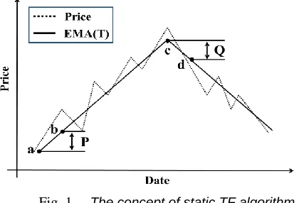
Static TF algorithm was proposed by Fong et al. [5]. The main idea of static TF algorithm is to smooth the price data by using Exponential Moving Average (EMA) and determine the trading timing based on a pair of thresholds P and Q. Threshold P (Q) is the vertical length of an upward (downward) EMA. Threshold P is used for opening a position and threshold Q is used for closing the opened position. Threshold P and Q are static constants and their optimal values can be manually set by the traders or obtained from the study of historical price data. The concept of thresholds P and Q is depicted in Figur-1 and the pseudo-code of static TF algorithm is given in Algorithm-1. For the example in Figure-1, a position will be opened at time point b and closed at time point d.
2.2 Adaptive TF Algorithm
In adaptive TF algorithm, the thresholds P t and Qt are variables instead of static constants. The values of thresholds P t and Qt are dynamically changed according to the market trend. Adaptive TF algorithm utilizes EMA and RSI technical indicators. Furthermore, the concept of thresholds in an adaptive TF algorithm is also different from the static one. In adaptive TF algorithm, threshold Pt is a set of criteria to open a long position and close out a short position. Likewise, threshold Qt is a set of criteria to open a short position and close out a long position. The pseudo-code of adaptive TF algorithm is given in Algorithm 2.
Fig. 1. The concept of static TF algorithm
Algorithm-1: Static TF algorithm
Variable: upward turning point utp, downward turning point dtp
repeat
Compute EMA(t);
If EMA(t)>EMA(t−1)&&EMA(t−2)>EMA(t−1) then upt=EMA(t−1);
Current trend is an uptrend
elseif EMA(t)<EMA(t−1)&&EMA(t−2)<EMA(t−1) then dtp=EMA(t−1);
Current trend is a downtrend end
if no position is opened && current trend is uptrend then if EMA(t) – utp ≥ P then
Open aposition end
else if the position is opened && current trend is downtrend then
if dtp−EMA(t)≥Q then Close the position end
end
if at the end of market then Close the opened position end
until at the end of market; Algorithm-2: Adaptive TF algorithm
repeat
Compute RSI(t) and RSI(EMA(t)); If RSI(t) >50then
current trend is a uptrend else if RSI(t) <50 then current trend is a down trend
end if RSI(t) >RSI(EM A(t)) &&40 <RSI(EM A(t)) >60 && current trend is a
uptrend&& no position is opened then Open a position, Pt
else if RSI(t) < RSI (EM A(t)) &&40 <RSI(EM A(t)) >60 && current
trend is a down trend && the position is opened then Close the opened position, Qt
end if at the end of market then Close the opened position end
until at the end of market;
All tables and figures will be processed as images. You need to embed the images in the paper itself. Please don’t send the images as separate files.
3 MULTI-THRESHOLD
TREND
FOLLOWING
ALGORITHM
One of the main objectives of this research is to devise a TF algorithm which can signal the right moment to purchase and sell shares. In addition, the algorithm should also avoid unprofitable transactions whenever possible. To achieve these objectives, five multi-threshold trend following algorithms are proposed in this section. These algorithms are constructed incrementally to address various shortcomings of the basic TF algorithm. These algorithms include:
i. TF with MACD Centerline Crossover. ii. TF with threshold P1 and Q1.
iii. TF with threshold P1, P2 and Q1, Q2., iv. Muti-threshold TF.
3.1 TF with MACD Centreline Crossover
3748
idea of static TF algorithm is to smooth the price data by using Exponential Moving Average (EMA) and determine the trading timing based on a pair of thresholds P and Q. Threshold P (Q) is the vertical length of an upward (downward) EMA. Threshold P is used for opening a position and threshold Q is used for closing the opened position. Threshold P and Q are static constants and their optimal values can be manually set by the traders or obtained from the study of historical price data. The concept of thresholds P and Q is depicted in Figur-1 and the pseudo-code of static TF algorithm is given in Algorithm-1. For the example in Figure-1, a position will be opened at time point b and closed at time point d.
3.2 Technical indicators
3.2.1 Moving Averages
Technical indicators translate price information into simple, easy-to-read signals. So far, several technical indicators have been developed by analysts. Moving averages are the most basic and useful technical indicators. Moving averages smooth the price data to identify the current market direction with a lag. Moving averages have a certain lag because they are based on historical price data. Two well-known moving averages are Simple Moving Average (SMA) and Exponential Moving Average (EMA). SMA is formed by computing the average price of a security at any given time. The calculation of SMA is given in Equation 1, where t and n are transaction day and time interval.
Fig. 2. The idea of TF
(1) EMA reduces the lag by applying more weight to recent prices. The weight applied to the most recent price depends on the number of periods in the moving average. As a result, EMA is more sensitive to latest changes of prices than SMA. To calculate EMA, a SMA is used as the previous period’s EMA in the first calculation. The calculation of EMA is given in Equation 2, where t and n are transaction day and time interval.
(2) Moving Average Convergence Divergence:
Developed by Gerald Appel [1] in the late seventies, the Moving Average Convergence Divergence (MACD) is one of the simplest and most effective momentum indicators. In a stock market, momentum is the measurement of speed or
velocity of prices changes. MACD can not only determine the strength the current trend but also indicate when the trend is in danger of losing momentum. According to Alexander Elder [4], the MACD indicator has the following architecture:
i. Long-term average: EMA of 26 days for share price ii. Short-term average: EMA of 12 days for share price iii. Signal line: EMA of 9 days of the MACD itself
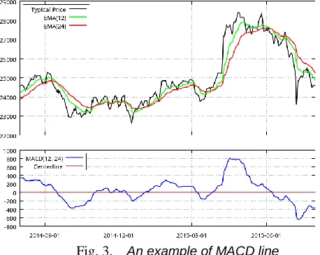
The values of 12, 26 and 9 are the typical settings used with the MACD. However other values can be substituted depending on the trading style and goals. The MACD line turns two moving averages into a momentum oscillator by subtracting the long-term moving average from the short-term moving average. In Figure 3, the MACD line fluctuates above and below the zero line, which is also known as a centerline. MACD however, could not identify overbought and oversold since the value of MACD is unbound.
The calculation of MACD line is given in Equation 3, where t, EMAs and EMAl are transaction day, short-term EMA and long-term EMA.
(3) It is worth stressing that, MACD line reflects the speed of price changes, rather than the change of price. Four different periods in Figure 4 are classified as follows: From time point A to time point B, the MACD is negative and the downside momentum is increasing. It means that current trend is downtrend and this downtrend will continue for a certain period of time. From time point B to time point C, the MACD is negative and the downside momentum is decreasing. It means that current trend is downtrend and this downtrend is likely to reverse soon. From time point C to time point D, the MACD is positive and the upside momentum is increasing. It means that current trend is uptrend and this uptrend will continue for a certain period of time.
Fig. 3. An example of MACD line
3749
price is rising when the value of MACD line is positive. Bullish centerline crossover can be considered as the signal of the establishment of an uptrend. A bearish centerline crossover occurs when the MACD line moves below the centerline to turn negative. This case happens when the 12 days EMA moves below the 26 days EMA. The share price is falling when the value of MACD line is negative. Bearish centerline crossover can be identified as the signal of the termination of the prior uptrend. From what we discussed above, the buy and sell signal can be generated based on MACD CC. The rules for buy and sell signal generations are listed as follows and the pseudo-code of TF with MACD CC is given in Algorithm 3. Buy in when a bullish centerline crossover occurred, Sell out when a bearish centerline crossover occurred.
Fig. 4. Four different periods in MACD
Algorithm 3: TF with MACD CC Compute MACD(t);
repeat
if MACD(t) >0 && MACD(t − 1) <0 && no position opened then open a position
end
if MACD(t) <0 && MACD(t − 1) >0 && a position is opened then close the position
end
if At the end of simulation && a position is opened then Close the position
end
until at the end of simulation;
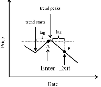
From our extensive testing on TF with MACD CC, we find that the algorithm tends to follow weak uptrend which results in unprofitable transactions. Figure 5 depicts the scenario of following a weak uptrend by TF with MACD CC. In Figure 5, a buy signal is generated at time point A because a bullish center line crossover is detected. Likewise, its subsequent sell signal is generated at time point B because a bearish centerline crossover is detected. However, we can notice that this transaction is unprofitable since the uptrend is ended soon after time point A. Therefore, success rate (SR) of transactions can be improved if the TF algorithm ignores weak uptrend and only follows strong uptrend. To alleviate this problem, a TF with threshold P1 and Q1 is proposed in the next section.
3.3 TF with thresholds P1and Q1
As shown in Figure 6, trends can be classified into four categories. It is easy to identify uptrend and downtrend by the use of MACD; positive MACD represents uptrend and negative MACD represents downtrend. MACD can be used to determine how strong the trend is. High positive MACD represents strong uptrend and low negative MACD represents
strong downtrend. In order to identify strong and weak uptrend, a pair of MACD thresholds P1 and Q1 is proposed for trend following. P1 is a level of positive MACD and Q1 is a level of negative MACD. If the MACD line crosses above (below) the threshold P1 (Q1), the trend can be considered as a strong uptrend (downtrend), otherwise the trend is considered as a weak uptrend (downtrend).
Fig. 5. Following weak uptrend in TF with MACD CC
The rules used to identify strong and weak trend is based on a theory that a strong uptrend (downtrend) has a strong upside (downside) momentum. Thresholds P1 (Q1) actually is the levels to identify strong and weak upside (downside) momentums. Figure 6 depicts the concept of thresholds P1 and Q1 and the MACD line does not cross above threshold P1 until time point A. The uptrend which takes place before time point A is identified as a weak uptrend. Since time point A can be considered as the timestamp of a strong uptrend establishment, a buy signal will be generated at time point A. The MACD line does not cross below threshold Q1 until time point B. The downtrend which takes place before time point B is identified as a weak downtrend. However, the weak downtrend does not necessarily indicate that the prior strong uptrend has been already ended. Therefore, a sell signal will not be generated until time point B. At time point B, the downtrend is considered as a strong downtrend and it also indicates that the prior strong up trend is already ended.
Fig. 6. The concept of threshold P1 and Q1
3.4 Algorithm design for TF with thresholds P1 and Q1
3750
downtrend indicates that the prior strong uptrend is already ended.
Algorithm 4: TF with P1 and Q1
Repeat
Compute MACD(t);
if MACD(t − 1) < P1 && M ACD(t) > P1 && no position opened then
Open a position end
if MACD(t − 1) > Q1 && M ACD(t) < Q1 && a position is opened then
Close the position end
if At the end of simulation && a position is opened then close the position
end
Until at the end of simulation;
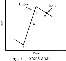
Although TF with threshold P1 and Q1 is effective to improve SR, we find that it cannot handle stock slump and soar. In a stock slump, the price takes a nose dive and in a stock soar, the price rises sharply. Figure 8 illustrates stock slump and soar.
Fig. 7. Stock soar
In figure 7, the price rose rapidly from time point A. A bullish centerline crossover occurred at time point B and the MACD line crossed above threshold P1 at time point C. Therefore, the buy signal was not generated until time point C. The subsequent sell signal was generated at time point D. However, this transaction can be profitable if the buy signal was generated before time point B.
Fig. 8. Stock slump
In figure 8, a buy signal was generated at time point A and then the price dropped rapidly from time point B. A bearish centerline crossover happened at time point C and the MACD line crossed below threshold Q1 at time point D. Therefore, the sell signal was not generated until time point D. However, this transaction can be profitable if the sell signal was generated before time point C.. However, in the case of stock soar (see
Figure 10b), downside momentum decreases rapidly and may not fell back. Similarly, Figure 11 one depicts the decreasing upside momentum in normal case and other one depicts the decreasing upside momentum during stock slump where it decreases rapidly.
4 RESULT
AND
DISCUSSION
In order to evaluate the performance of TF algorithms, seven well-known stock indexes listed in Table-1 are chosen as experiment data. The historical inter-day typical price is used for the experiments. Dataset is divided into training and testing data. The training data is from 01/08/2011 to 31/07/2014 (3 years) and the testing data is from 01/08/2014 to 31/07/2015 (1 year). Typical price (TP) refers to the arithmetic average of the high, low, and closing price for a given period in financial trading [17], it can be calculated as shown in Equation 6. The function of typical price is to smooth daily price fluctuation.
(6)
Table-I: Name of the Table that justifies the values
Stock symbol Stock index
IXIC NASDAQ Composite
SP500TR S&P 500(TR) HIS Hang Seng index
TWII TSEC weighted index
FTSE FTSE100
DJI Dow Jones
N225 Industrial Average Nikkei 225
In our experiments, Success Rate (SR) is used to evaluate the quality of transaction. SR is the proportion of profitable transactions. The calculation of SR is given in Equation 7. Accumulated Return on Investment (AROI) is used to evaluate the quality of transactions and it can be calculated as shown in Equation 8, where buy (i, t) and sell (i, tt) are the buying and selling price of the ith transaction. A transaction comprises of a buy action and a subsequent sell action. t and tt are the transaction day of these two actions respectively. N is the total number of transactions recorded in the entire trading session.
(7)
(8)
4.1 Experiment on TF with MACD CC
3751
transactions in TF with MACD CC follow the weak uptrend and could be unprofitable. Due to the limited space, we will only show the transactions from HSI dataset in the following experiments. Transactions from remaining 6 stock indexes can be analyzed in a similar way.
Table-II: Experiment result of TF with MACD CC
Testing Session
Stock index TT PT SR AROI
IXIC 5 3 60.00% 6.69%
SP500 9 2 22.22% -8.47%
HIS 4 2 50.00% 7.37%
TWII 4 1 25.00% -1.69%
FTSE 6 1 16.67% -5.54%
DJI 8 2 25.00% -7.75%
N225 4 3 75.00% 16.62%
Average 5.71 2.00 35.00% 1.03%
Fig. 9. TF with MACD CC in HIS
Table-III: The details of transactions from Figure-9
Sl. No. Date to buy Buying price
Date to sell Selling price
Profit ROI 1 2014-11-04 23892.64 2014-11-21 23415.53 -477.11 -2.00% 2 2014-11-24 23884.34 2014-12-11 23288.34 -595.91 -2.49% 3 2015-01-05 23791.90 2015-03-09 24079.69 287.79 1.21% 4 2015-03-27 24485.51 2015-06-09 27094.41 2608.90 10.65%
Total 1823.67 7.37% 4.2 Experiment on TF with thresholds P1and Q1
The optimal values of thresholds P1 and Q1 are found by PSO in the training session. The buy and sell signals are generated in the testing session based on these thresholds. Next, we calculate the SR and AROI of these transactions generated in the testing session. Table 4 lists the optimal values of thresholds P1 and Q1 and Table 5 shows the experiment results of TF with threshold P1 and Q1. In Table 5, TT denotes the total number of transactions and PT is the total number of profitable transactions. From Table 2 and Table 5, we can observe that the SR is improved in TF with threshold P1 and Q1 (from 35.00% to 53.85%). AROI is also increased (from 1.03% to 3.85%) since the proportion of unprofitable
transaction is reduced.
Table-IV: The optimal values of thresholds P1 and Q1
Stock index Range of P1 Range of Q1 P1 Q1 IXIC [0, 33.07] [-31.81, 0] 17.92 -31.81 SP500 [0, 14.34] [-11.47, 0] 8.19 -11.47 HSI [0, 227.69] [-303.81, 0] 104.68 -274.20 TWII [0, 85.03] [-94.72, 0] 68.03 -27.99 FTSE [0, 52.04] [-53.84, 0] 0.31 -33.06 DJI [0, 121.8] [-122.97, 0] 16.89 -111.07 N225 [0, 156.89] [-145.77, 0] 55.81 -116.95
Table-V: Results of TF with thresholds P1 and Q1
Training session
Testing session Stock index PT SR TT PT SR AROI
IXIC 4 100.00% 2 1 50.00% 6.22% SP500 4 100.00% 2 1 50.00% 0.64% HSI 4 80.00% 1 1 100.00% 8.32% TWII 4 80.00% 1 1 100.00% 2.28% FTSE 4 44.44% 3 1 33.33% -6.09% DJI 5 100.00% 2 1 50.00% -1.70% N225 4 80.00% 2 1 50.00% 17.30%
Average 1.8
6
1.00 53.85% 3.85%
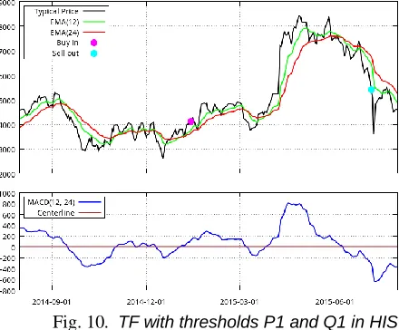
Figure 10 depicts the transactions on HSI during the testing session (from 01/08/2014 to 31/07/2015) when TF with threshold P1 and Q1 is employed. Table 6 lists the details of the transactions from Figure 10. From Table 6, we can observe that only one transaction is recorded in the testing session. It also reveals that the algorithm attempts to follow strong uptrend in this case. The experiment results confirm that TF with thresholds P1 and Q1 achieve our intended objective; to ignore weak uptrend and to follow strong uptrend.
Fig. 10. TF with thresholds P1 and Q1 in HIS
4.3 Experiment on TF with thresholds P1, P2and Q1, Q2
3752
Figure-16, depicts the transactions on HSI during the testing session (from 01/08/2014 to 31/07/2015) when TF with threshold P1, P2 and Q1, Q2 is employed. From Table 3 and Table 6, we can observe that TF with thresholds P1, P2 and Q1, Q2 is shown to be sensitive to the stock slump which happened from May to July 2015 in HSI. The exact date of responding to the stock slump in HSI by each TF algorithm is given in Table-XI.
Table-VI: The search spaces of thresholds P1, P2, Q1 and Q2
Stock index Range of P1 Range of Q1 Range of P2 Range of Q2 IXIC [0, 33.07] [-31.81, 0] [0, 89.66] [0, 63.33] SP500 [0, 14.34] [-11.47, 0] [0, 40.71] [0, 25.10] HSI [0, 227.69] [-303.81, 0] [0, 802.03] [0, 524.00] TWII [0, 85.03] [-94.72, 0] [0, 300.55] [0, 217.19] FTSE [0, 52.04] [–53.84, 0] [0, 193.53] [0, 100.60] DJI [0, 121.8] [-122.97, 0] [0, 345.03] [0, 223.52] N225 [0, 156.89] [-145.77, 0] [0, 361.33] [0, 607.99]
Table VII: The optimal values of thresholds P1, P2 and Q1, Q2
Stock index P1 Q1 P2 Q2
IXIC 28.14 -22.82 61.61 8.43 SP500 0.75 -11.44 33.11 22.82 HIS 135.46 -297.10 529.44 313.13 TWII 69.33 -69.11 213.17 62.95 FTSE 0.98 -47.22 5.1 0 41.76 DJI 40.65 -121.43 54.39 218.94 N225 106.66 -100.33 159.41 581.92
Table-VIII: Results of TF with threshold P1, P2 and Q1, Q2
Training Session Testing Session Stock
index
TT PT SR TT PT SR AR
OI
IXIC 8 8 100.00
%
4 3 75.00% 5.8 9%
SP500 4 4 100.00
%
2 1 50.00% 2.4 7%
HSI 4 4 100.00
%
1 1 100.00 %
13. 25 %
TWII 4 4 100.00
%
1 1 100.00 %
1.9 5%
FTSE 9 9 100.00
%
5 2 40.00% -0.6 5%
DJI 5 5 100.00
%
2 1 50.00% 3.9 1%
N225 6 5 83.33% 3 2 66.67% 16.
80 %
Average 2.5
7 1.5 7
61.11% 6.2 3%
Table-IX: The exact dates of responding to the stock slump in HSI of each TF algorithm
TF algorithm Selling date Selling price TF with MACD CC 2015-06-09 27094.41
TF with P1 and Q1 2015-07-03 26133.36 TF with P1, P2 and Q1,
Q2
2015-05-07 27367.25
Fig. 11. TF with threshold P1, P2 and Q1, Q2 in HSI
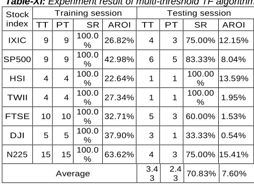
Table- 10 lists the values of threshold P1, P2 and Q1, Q2, found for optimizing both SR and AROI. In testing session, the buy and sell signals are generated based on the optimal values of the thresholds. The experiment result of multi-threshold TF algorithm is given in Table 16. TT denotes the total number of transactions and PT is the total number of profitable transactions. From Table 14 and Table 16, we can observe that the SR is increased by 3.89% (from 68.18% to 70.83%) and AROI is increased by 14.11% (from 6.66% to 7.60%).
Table-X: The threshold P1, P2 and Q1, Q2 for SR and AROI
Stock index P1 Q1 P2 Q2 IXIC 32.7
8 -20.17 14.50 6.50 SP500 14.1
7 -11.21 2.33 6.43
HSI 85.2
7
-303.81 395.73 519.55 TWII 71.7
6 -69.03 153.14 65.46 FTSE 4.30 -49.12 4.86 41.91
DJI 111.
33
-116.66 34.15 165.36 N225 27.3
5
-145.17 15.84 1.24
Table-XI: Experiment result of multi-threshold TF algorithm
Stock index
Training session Testing session TT PT SR AROI TT PT SR AROI IXIC 9 9 100.0
% 26.82% 4 3 75.00% 12.15% SP500 9 9 100.0% 42.98% 6 5 83.33% 8.04%
HSI 4 4 100.0
% 22.64% 1 1
100.00
% 13.59% TWII 4 4 100.0
% 27.34% 1 1
100.00
% 1.95% FTSE 10 10 100.0
% 32.71% 5 3 60.00% 1.53% DJI 5 5 100.0
% 37.90% 3 1 33.33% 0.54% N225 15 15 100.0
% 63.62% 4 3 75.00% 15.41%
Average 3.4
3 2.4
3753 4.4 Comparison with other TF algorithms
In this section, we compare the multi-threshold TF algorithm with static TF, adaptive TF, and FGA based TF.
4.4.1 Comparison with static TF algorithm
The values of thresholds P and Q in static TF algorithm can be manually set by the users. In this experiment, we use ten pairs of thresholds P and Q ([(P=10, Q=10), (P=20,Q=20), (P=30,Q=30), (P=40,Q=40), (P=50,Q=50), (P=60,Q=60), (P=70,Q=70), (P=80, Q=80), (P=90, Q=90), (P=100, Q=100)]) to evaluate the static TF algorithm. The experiment results of static TF algorithm are listed below tables.
Table-XII: Experiment result of static TF algorithm
Stock index
Testing session
P=30 and Q=30 P=40 and Q=40 TT
S PT SR AROI TTS PT SR AROI IXIC 7 3 42.86
% 0.30% 5 2 40.00
% 2.99% SP500 4 1 25.00
% -3.99% 2 1 50.00
% 1.73% HSI 11 4 36.36% 5.72% 11 4 36.36% 2.60% TWII 5 2 40.00
% -1.39% 5 2 40.00
% -3.44% FTSE 7 2 28.57
% -6.99% 7 2 28.57
% -11.60% DJI 10 3 30.00% -0.54% 9 4 44.44% -2.99% N225 10 5 50.00
%
19.96
% 8 5
62.50
% 18.60% Average 7.71 2.86 37.04% 1.87% 6.71 2.86 42.55% 1.13%
Table-XIII: Experiment result of static TF algorithm
Stock index
Testing session
P=50 and Q=50 P=60 and Q=60 TTS PT SR AROI TTS PT SR AROI IXIC 4 2 50.00
% 4.53% 4 2 50.00% 3.31% SP500 2 1 50.00% -1.10% 1 1 100.00% 4.36%
HSI 11 3 27.27
% -2.54% 11 3 27.27% -4.46% TWII 5 2 40.00
% -3.76% 4 2 50.00% -0.60% FTSE 7 1 14.29
% -13.04% 5 1 20.00% -6.20% DJI 8 3 37.50
% -3.68% 8 2 25.00% -4.56% N225 8 4 50.00
% 16.60% 7 4 57.14% 19.59%
Averag
e 6.43 2.29 35.56
% -0.43% 5.71 2.14 37.50% 1.63%
Table-XIV: Experiment result of static TF algorithm Table-XV: Experiment result of static TF algorithm
Stock index
Testing session
P=70 and Q=70 P=80 and Q=80 TTS PT SR AROI TTS PT SR AROI IXIC 3 1 33.33% 8.47% 3 1 33.33% 3.90% SP500 1 1 100.00% 4.26% 1 1 100.00% 3.97%
HSI 10 3 30.00% -5.78% 9 2 22.22% -3.45% TWII 3 1 33.33% 1.28% 3 1 33.33%
-1.16% FTSE 5 2 40.00% -7.28% 5 1 20.00% 7.27%
-DJI 8 1 12.50% -7.53% 8 2 25.00% -7.80% N225 7 5 71.43% 19.43% 6 5 83.33% 21.02
% Average 5.29 2.00 37.84% 1.82% 5.00 1.86 37.14% 1.32%
a) Comparison with adaptive TF algorithm
Table-17 lists the experiment result of adaptive TF algorithm.
Comparison with FGA based TF. TF with FGA uses a pair of thresholds P and Q to generate buy and sell signals. The objective of FGA is to search the optimal values of thresholds P and Q. In TF with FGA, average return from Equation 14 is used as the fitness function, where buy (i, t) and sell (i, tt) are the buying and selling price of ith transaction. A transaction comprises a buying and a succeeding selling action. t and tt are the timestamps of these two actions respectively.
Table-XVI: Experiment result of static TF algorithm
Stock index
Testing session
P=90 and Q=90 P=100 and Q=100 TTS PT SR AROI TTS PT SR AROI IXIC 3 1 33.33% 4.88% 3 1 33.33% 3.97% SP50
0
1 1 100.00 %
3.49% 1 1 100.00% 3.33% HSI 7 2 28.57% 1.46% 7 2 28.57% 2.11% TWII 3 1 33.33% 0.73% - 3 1 33.33% -1.12% FTSE 5 1 20.00%
-10.75%
4 0 0.00% -8.53%
DJI 6 1 16.67% -4.74%
6 1 16.67% -5.29%
N225 6 4 66.67% 20.99% 6 4 66.67% 19.43% Average 4.43 1.57 35.48% 2.09% 4.29 1.43 33.33% 1.99%
Table-XVII: Experiment result of adaptive TF algorithm
Stock index Testing session
TTS PT SR AROI
IXIC 7 4 57.14% 3.91%
SP500 10 4 40.00% -2.84%
HSI 7 2 28.57% 6.14%
TWII 6 2 33.33% -8.40%
FTSE 8 2 25.00% -3.80%
DJI 8 1 12.50% -3.58%
N225 4 3 75.00% 17.55%
Average 7.14 2.57 36.00% 1.28% Stock
index
Testing session
P=10 and Q=10 P=20 and Q=20 TTS PT SR AROI TTS PT SR AROI IXIC 10 4 40.00% 1.11% 8 3 37.50% -1.28% SP500 9 1 11.11% -8.77% 5 1 20.00% -4.96% HSI 14 5 35.71% 7.96% 12 5 41.67% 8.34% TWII 10 4 40.00% -1.23% 6 2 33.33% 2.45% FTSE 10 3 30.00% -1.13% 8 2 25.00% -7.84% DJI 15 3 20.00% 2.24% 11 4 36.36% 2.59% N225 13 7 53.85% 24.81
% 10 5 50.00% 22.94% Averag
e 11.5
7 3.8
6 33.33% 3.57% 8.57 3.1
3754
N is the total number of transactions recorded in the entire trading session. For comparison, the SR and AROI of transactions occurred during the testing session are computed.
In TF with FGA, the time interval of EMA and the ranges of threshold P and Q can e input by the users based on the desired level of risk. We set the time interval of EMA to be 12 days. The range of threshold P (Q) is set to the max vertical distance of the uptrend (downtrend) in the training sesson. In this experiment, PSO is used for searching optimal values of threshold instead of FGA because PSO can achieve similar result. Table 18 lists the best values of threshold P and Q found by the algorithm and Table 20 lists the experiment result Overall comparison: The overall experiment results of five TF algorithms ((1) TF with MACD Centerline Crossover, (2) TF with threshold P1 and Q1, (3) TF with threshold P1, P2 and Q1, Q2, (Muti-threshold TF) are given in Table 20. Figure14 shows the SR and AROI
Table-XVIII: The thresholds P and Q in TF with FGA
Stock index Range of
P Range of Q P Q
IXIC [0, 376.72] [0, 217.06] 12.7 217.06 SP500 [0, 135.77] [0, 64.84] 3.26 64.84
HSI [0, 2932.61] [0, 2471.12] 310.65 2471.12 TWII [0, 984.22] [0, 442.32] 148.72 442.32 FTSE [0, 396.35] [0, 450.74] 3 450.74 DJI [0, 1019.75] [0, 773.49] 0 773.49 N225 [0, 2619.47] [0, 1705.17] 1437.59 247.14
Table-XIX: Experiment result of TF with FGA
3 TTS PT Avg. return SR AROI IXIC 2 1 5.58% 50.00% 11.17%
SP500 2 1 1.96% 50.00% 3.92%
HSI 1 0 -1.95% 0.00% -1.95%
TWII 1 0 -9.71% 0.00% -9.71%
FTSE 1 0 -0.34% 0.00% -0.34%
DJI 1 1 6.52% 100.00% 6.52%
N225 2 0 -1.71% 0.00% -3.42%
Average 1.43 0.43 0.05% 28.57% 0.88%
For each stock index and Figure 13 shows the AROI for each stock index by different TF algorithm. Figure 14 depicts the results of SR and AROI when the multi-threshold TF is compared to static, dynamic, and float encoding genetic algorithm based TF. From Figure 14, we can observe that the proposed multi-threshold achieves the best overall results among all TF algorithms.
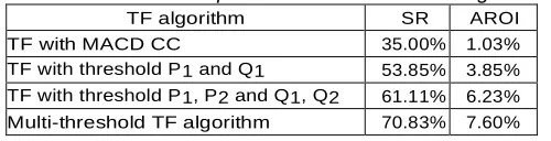
Table-XX: The overall experiment results of our TF algorithms
TF algorithm SR AROI
TF with MACD CC 35.00% 1.03%
TF with threshold P1 and Q1 53.85% 3.85% TF with threshold P1, P2 and Q1, Q2 61.11% 6.23% Multi-threshold TF algorithm 70.83% 7.60%
5 CONCLUSION
A novel multi-threshold TF algorithm is proposed in this paper. In this algorithm, three pairs of thresholds are designed to address various issues on different working regions. The effective region of each threshold is separated by MACD and
the function of each threshold can be summarized as follows: Threshold P1 identifies the strong and weak uptrends after MACD bullish centerline crossover. Threshold Q1 identifies the strong and weak downtrends after MACD bearish centerline crossover. Threshold P2 detects stock soar before MACD bullish centerline crossover. Threshold Q2 detect stock slump before MACD bearish centerline crossover. Threshold P3 identifies strong and weak uptrends at MACD bullish centerline crossover. Threshold Q3 identifies strong and weak downtrends at MACD bearish centerline crossover.
The search spaces of thresholds and parameters are resolute from the price data as an alternate of being input by the users to reduce human bias. The performance of the algorithm was tested on 7 well-known indexes from various stock markets. Experimental results show that the proposed algorithm achieves the best result in maximizing SR and AROI when it is compared with static TF, dynamic TF, and TF with Float Encoding Genetic algorithms.
Fig. 12. SR for each stock index
Fig. 13. AROI for each stock index
(a) SR comparison (b) AROI comparison
Figure 14: Overall comparison
3755
proposed multi-threshold TF algorithm is able to identify unprofitable weak uptrends and capable of responding to stock soar and slump in trend following. The experiment results also reveal that the proposed approach can determine the strength of uptrends and downtrends in trend following. As regards the future dimension of the study, we are planning to extend the current algorithm with an Artificial Neural Network (ANN) for recognizing additional market situations.
7.3 REFERENCES
[1] Appel, G.(1985).The Moving Average Convergence-Divergence Trading Method.(advanced ed.). Traders Pr. [2] A.S, S. (2013). A study on fundamental and technical
analysis. International Journal of Mar- keting, Financial Services & Management Research, 2, 44–59.
[3] Covel, M. W. (2009) Trend Following: Learn to Make Millions in Up or Down Markets. (Up- dated ed.). Upper
Saddle River, New Jersey 07458: Pearson
EducationLimited.
[4] Elder, A. (1993) trading for a living: psychology, trading tactics, money management. John Wiley & Sons, Inc. [5] Fong, S., Si,Y.-W., & Tai, J.(2012).Trend following
algorithms in automated derivatives market trading. Expert Systems with Applications , 39 ,11378–11390.
[6] Fong, S., Tai, J., & Si, Y. W. (2011). Trend following algorithms for technical trading in stock market. Journal of emerging technologies in web intelligence, 3, 136–145.
[7] Investopedia (2016). Overbought.
http://www.investopedia.com/terms/o/overbought.asp. Accessed: 2016-05-18.
[8] Investopedia (2016). Oversold.
http://www.investopedia.com/terms/o/oversold.asp. Accessed: 2016-05-18.
[9] Kameyama, K. (2009). Particle swarm optimization - a survey. IEICE Transactions on Information and Systems, E92-D ,1354–1361.
[10] Kennedy, J., & Eberhart, R. (1995). Particle swarm optimization. In IEEE International Conference on Neural Networks (pp. 1942–1948). IEEE volume4.
[11] Luo, J., Si, Y.-W., &Fong, S. (2012). Trend following with float-encoding genetic algorithm. In Digital Information Management (ICDIM) (pp. 173–176). IEEE.
[12] Machado, J., Neves, R., & Horta, N. (2015). Developing multi-time frame trading rules with a trend following strategy, using GA. In GECCOCompanion’15 Proceedings of the Companion Publication of the 2015 Annual Conference on Genetic and Evolutionary Computation (pp.765– 766). ACM.
[13] Murphy, J. J. (1999). Technical analysis of the financial markets: a comprehensive guide to trading methods and applications. (2nd ed.). New York: New York Inst. of Finance.
[14] Nguyen, D., Yin, G., & Zhang, Q. (2013). Trend-following trading using recursive stochastic optimization algorithms. In 52nd IEEE Conference on Decision and Control (pp.7827–7832). IEEE.
[15] Wikipedia (2016). Bernard baruch
https://en.wikipedia.org/wiki/Bernard_Baruch. Accessed: 2016-06-11.
[16] Wikipedia (2016). Typical price.
https://en.wikipedia.org/wiki/Typical_price. Accessed: 2016-05-21.
[17] Wilder, J. W. (1978). New Concepts in Technical Trading Systems. Trend Research.