DETERMINATION OF SPINODAL POINTS IN
EQUATION OF STATE USING NON LINEAR
OPTIMIZATION SQP METHOD IN MULTIPHASE
FLOW
Deepak Awasthi
1, Ashutosh Tiwari
2, Rajive Gupta
3 1Department of Mechanical Engineering,
2Department of Applied Physics,
Pranveer Singh Institute of Technology, Kanpur (India)
3
Department of Mechanical Engineering, Harcourt Butler Technological Institute, Kanpur (India)
ABSTRACT
To solve multiphase flow among various models D2Q9 Lattice Boltzmann model is found to be very much
effective. In order to apply this model the equation of state of fluid under consideration is to be known. In this
EOS the proper detection of metastable region is a very important issue. This metastable region lies between
two spinodal points having densities ρ1 and ρ2 . Values of ρ1 and ρ2 can be obtained by solving the conditions of
Mechanical and Chemical equilibrium. In the present study for the proper evaluation of these points Sequential
Quadratic Programing (SQP)method is used, which gives better prediction of the values of ρ1 and ρ2 as
compared to the same values calculated by other previous workers.
Keywords: Chemical Equilibrium, Equation of State, Mechanical Equilibrium, Multiphase Flow,
Sequential Quadratic Programming
In oil and gas industry, it is important to meter the individual components of oil, water and gas stream. This will
therefore focus on hydrocarbon multiphase flow measurement. Although multiphase flows also exist in other
industries, the term multiphase flow is used to refer to any fluid flow consisting of more than one phase or
component.
I. INTRODUCTION
In every processing technology multiphase flow exist starting from cavitating pumps and turbines to
electrophotographic processes to papermaking to the pellet form of almost all raw plastics. The amount of
granular material, coal, grain, ore, etc. that is transported every year is enormous and, at many stages, that
material is required to flow. Clearly the ability to predict the fluid flow behavior of these processes is the
effectiveness of those processes. Multiphase flows are also a ubiquitous feature of our environment whether one
considers rain, snow, fog, avalanches, mud slides, sediment transport, debris flows, and countless other natural
phenomena. Biological and medical flows like blood flow and semen are also multiphase. Two general
flows. Disperse flows mean those consisting of finite particles, drops or bubbles (the disperse phase) distributed
in a connected volume of the continuous phase. On the other hand separated flows consist of two or more
continuous streams of different fluids separated by interfaces. A multiphase system can contain the same
component with different phases such as liquid water and water vapor system. [1, 2]
II. D2Q9 LATTICE BOLTZMANN MODEL
The Lattice Boltzmann method was originated from Ludwig Boltzmann's kinetic theory of gases. The
fundamental idea is that gases/Fluids can be imagined as consisting of a large number of small particles moving
with random motions. The exchange of momentum and energy is achieved through particle streaming and
billiard-like particle collision. This process can be modelled by the Boltzmann transport equation [3]. The LBM
simplifies Boltzmann's original idea of gas dynamics by reducing the number of particles and connecting them
to the nodes of a lattice. For a two dimensional model, a particle is restricted to stream in a possible of 9
directions, including the one staying at rest. These velocities are referred to as the microscopic velocities and
denoted by where i = 0…………...8.
This model is commonly known as the D2Q9 model as it is two dimensional and involves 9 velocity vectors.
Figure1 shows a typical lattice node of D2Q9 model with 9 velocities and is defined by
= (1)
For each particle on the lattice, we associate a discrete probability distribution function = which
describes the probability of streaming in one particular direction.
The (D2Q9) Lattice Boltzmann model, i.e. two dimensional nine velocity LB model with a multiple relaxation
time (MRT) collision operator is considered. The extensive details of D2Q9 model is given in next section. The
MRT Lattice Boltzmann equation is given by [4]
(2)
Where ᴧ = is the diagonal matrix,
ᴧ = (3)
M is the orthogonal transformation matrix, Fἀ showsthe forcing term in the space velocity. Taking the help of
the transformation matrix, the R.H.S of Eq. (2) can be rewritten as
Where I is the unit tensor, S is the forcing term in the moment space with (I – 0.5 ᴧ) S=MF, and the equilibrium
meq is given by,
meq = (5)
The streaming process of the MRT LB equation is given by
fἀ(x+eἀ , t+ ) = fἀ* (x, t) (6)
Where f* = M-1 m*. The macroscopic velocity and the density can be computed by
= , v= + F (7)
Here F = (Fx Fy) is the force of interaction
F= - Gψ(x) (8)
Where ψ is the pseudopotential, G is the interaction strength, and w are the weights, which can be
written as w (1) = 1/3 and w (2) = 1/12 for the nearest - Neighbor interactions on the D2Q9 lattice.
In the original psedopotential model of Shan-Chen, the pseudopotential is expressed as = o exp (- o /
), which is normally constrained to multiple flow of low density ratio. For obtaining high density ratios, the
pseudopotential can be chosen as
= (9)
where cs = (c/ ), the lattice sound speed and p ( ) defines an expected equation of state such as the
Carnahan-Starling equation of state. With such choice psedopotential model of LBM have to undergo the lack of thermal
potential because of the non-reliable densities put up by the model after the solution that was given by the
Maxwell construction. Again it was discovered that the thermal reliability can be maintained by slightly
changing the mechanical stability conditions and that can be installed through the improved forcing scheme.
For the pseudopotential model of MRT, an updated forcing scheme is given as by
where = (Fx2 + Fy2) and σ can be used to update the mechanical stability conditions.
III. EQUATION OF STATE
Piecewise linear equations of state for the non-ideal fluids was proposed by Colosqui et al. [5]
p( ) = (11)
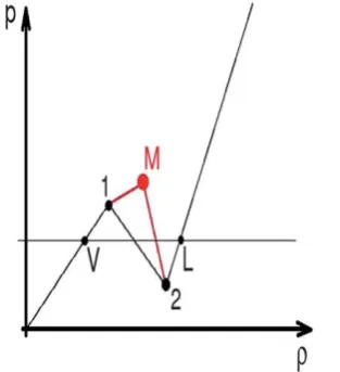
The concerned equation of state graph is shown in figure 01 in which there exists a clear relationship between
the pressure and the density of the droplet. It also explains the middle region or metastable region between the
state 1 and state 2 by point M.
Figure 01: Graph Showing Relationship Between Pressure (P) and Density (
)
in Equation of
State
Where V = (∂P/∂ )V , L = (∂P/∂ )L, and M = (∂P/∂ )M are the slopes of p( ) in the region of vapor phase,
liquid phase and the mechanically unstable area ( V>0 and L>0, whereas M < 0). Again, and are the
respective speed of sound of the corresponding vapor and liquid phases. The two unknown variables and
that express the spinodal points, are obtained by the solution of the following two simultaneous equations.
One is for the mechanical equilibrium
(12)
The second one for the chemical equilibrium
(13)
Where and are the density of the vapor and liquid respectively. It can be noted that for deriving the
Maxwell construction the following condition is used.
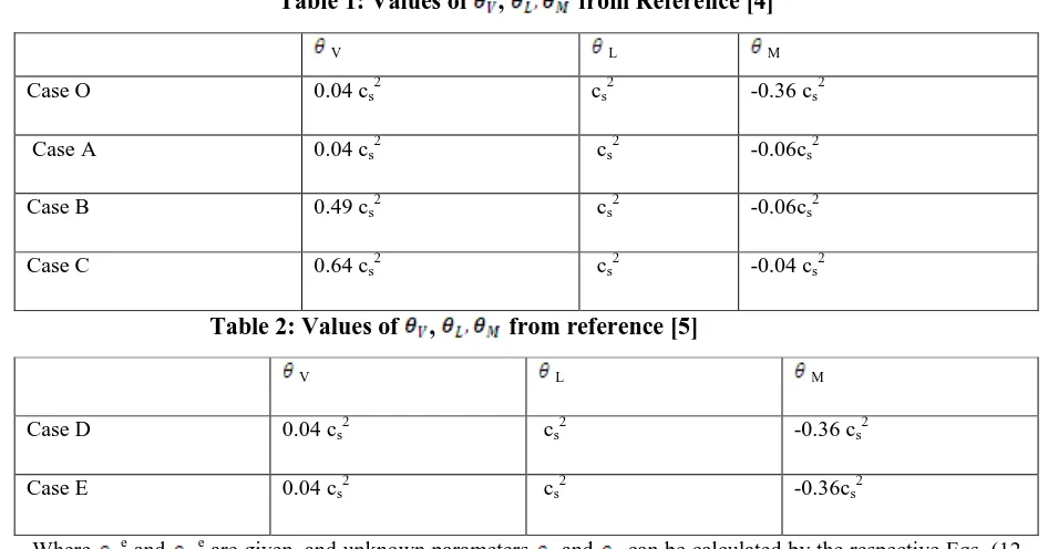
From reference [4], the parameters , can be taken as
Table 1: Values of
,
from Reference [4]
Table 2: Values of
,
from reference [5]
Where e and e are given, and unknown parameters and can be calculated by the respective Eqs. (12,
13).
The speed of the sound in the liquid phase is fixed and can empirically be given as ( L)1/2 = cs.
IV. SQP METHODOLOGY
The second equation of chemical equilibrium i.e. Eq. (13) is highly non linear that contains logarithmic
functions.
They can be written as,
= (15)
and
= (16)
In the above equations, , , and , are known quantities equations. Now a non linear programming
method is required to obtain the roots of above two equations.
According to Sequential Quadratic Programming (SQP) technique the roots of these equations (15) and (16) (i.e.
values of and ) will be obtained if the function of equation (15) i.e. and the function of equation (16)
i.e. satisfy the following conditions:
Min{ = 0 (17)
In order to solve the above mentioned equations by using SQP technique a computer code has been developed
using MATLAB [6].
V L M
Case O 0.04 cs2 cs2 -0.36 cs2
Case A 0.04 cs2 cs2 -0.06cs2
Case B 0.49 cs2 cs2 -0.06cs2
Case C 0.64 cs2 cs2 -0.04 cs2
V L M
Case D 0.04 cs2 cs2 -0.36 cs2
This condition is implemented via the function ‘fmincon’ provided in the optimization toolbox in MATLAB.
V. RESULTS
A comparative study between the minimum value of the function coming from the conditions using ‘fmincon’
and the minimum value of the same function by placing the conditions given in reference [4] and [5] are
compared in table 3.
Table3: Table Showing Values of
ρ
, ρ
min (F
12
+F
2 2)
for different values of ρ
l,
in all these cases ρ
v=
1.These values are compared with the values reported in reference [8].
ρl ρv ρ1,
(ref 5) ρ1, This work ρ2, (ref 5) ρ2, This work
min (F1
2
+F2
2 ),
(ref 5)
min (F1
2
+F2
2 ), This
work
10 1 5.32 5.3181 8.88 8.8878 1.2689e-004 6.0627e-008
100 1 34.29 34.2841 83.59 83.5838 4.0981e-005 1.3279e-007
1000 1 240.82 238.8636 806.09 805.5182 3.1360e-005 5.9003e-006
VI. CONCLUSION
The SQP optimization technique proves to be a better solver for such non linear problems as the values
suggested with the help of this method for the minimum of + predicts much lesser values as compare to
the values of the same function calculated by previous workers for the values of and suggested by them.
REFERENCES
[1]. A Textbook of Fundamentals of Multiphase Flows. California Institute of Technology Pasadena, Californi.
CambridgeUniversity press. 2005. Pg 01-410
[2]. Li. Chen, Q. Kang, Y. Mu, W. Q. Tao 2014. A critical review of the pseudopotential multiphase Lattice
Boltzmann Model, International journal of Heat and mass transfer. 76. Pg. 210-236
[3]. Chen, S. and Doolen, G. D. (1998) Lattice Boltzmann method for fluid flows. Annu. Rev. Fluid Mech., 30,
329–364.
[4]. Q. Li , K.H. Luo. 2014 Thermodynamic consistency of the pseudopotential lattice Boltzmann model for
simulating liquid vapor flows. Applied Thermal Engineering. 56-61
[5]. C. E. Colosqui, G. Falcucci, S. Ubertinib and S. Succi 2012.Mesoscopic simulation of non-ideal fluids
with self-tuning of the equation of state Soft Matter, 2012, vol 8, pg 3798.