Experimental, Numerical and Analytical Studies of the MHD-Driven Plasma Jet, Instabilities and Waves

(1)

MHD-driven plasma jet, instabilities and waves

Thesis by Xiang Zhai

In Partial Fulfillment of the Requirements for the Degree of

Doctor of Philosophy

California Institute of Technology Pasadena, California

2015

(2)

c

2015

(3)

Acknowledgements

I would like to express my most sincere gratitude to my adviser Prof Paul Bellan. Paul is an intelligent physicist with expertise in and a deep understanding of essentially all aspects of plasma physics and related fields, from theoretical analysis to experiment diagnostics, from circuit design to CAD drawing. He is an outstanding writer and speaker who knows how to use simple examples (like Los Angeles’ congested highways or South Park) to explain complex physics models. Paul is such a kind and patient mentor and friend, having a great sense of humor. Moreover, I could not appreciate more the interesting life experiences and adventures and stories Paul shared with the group. I am very fortunate to have Paul as my PhD advisor.

It is also a great pleasure to know Dr. Hui Li and Dr. Shengtai Li in Las Alamos National Lab and have Hui as a co-mentor in my PhD career. Hui is a brilliant astrophysicist and has a humble personality. He gave me a lot of valuable suggestions and guidance in both research topics and general academia career. Shengtai helped me learn how to run the numerical simulation code he and Hui developed. Since I worked primarily at Caltech and have multiple projects simultaneously, I always felt a little bit guilty because of my slow progresses in the Bellan group-Li group joint project. Now I also feel pity that I have to graduate, but there are so many more interesting and important topics we can study by involving both the lab experiment in Caltech and the numerical simulation in LANL. Fortunately we have Pakorn Tung Wongwaitayakornkul, a smart, hard-working, and productive young student who will take over the joint project. I can’t wait to see more exciting results.

(4)

(5)

great to see that the lab will remain in good shape.

Our group are so lucky to have Dave Felt, our professional electric engineering technician, and Connie Rodriguez, our responsible and warm-hearted secretary. Dave helped build plenty of facilities for the lab. I also gained a lot of valuable and helpful advices and suggestions from Dave when I was building the whistler probe and the HV probe. I can’t be more grateful to Connie for her patience in organizing the group’s office work, especially in handling the purchase orders from the group. Assuming that every group member averagely makes one purchase every week and we have about seven group members, that is one purchase everyday or∼400 purchases every year Connie has to take care of. She helps run the whole group smoothly.

(6)

Abstract

This thesis describes a series of experimental, numerical, and analytical studies involving the Caltech magnetohydrodynamically (MHD)-driven plasma jet experiment. The plasma jet is created via a capacitor discharge that powers a magnetized coaxial planar electrodes system. The jet is collimated and accelerated by the MHD forces.

We present three-dimensional ideal MHD finite-volume simulations of the plasma jet ex-periment using an astrophysical magnetic tower as the baseline model. A compact magnetic energy/helicity injection is exploited in the simulation analogous to both the experiment and to astrophysical situations. Detailed analysis provides a comprehensive description of the interplay of magnetic force, pressure, and flow effects. We delineate both the jet structure and the transition process that converts the injected magnetic energy to other forms.

When the experimental jet is sufficiently long, it undergoes a global kink instability and then a secondary local Rayleigh-Taylor instability caused by lateral acceleration of the kink instability. We present an MHD theory of the Rayleigh-Taylor instability on the cylindrical surface of a plasma flux rope in the presence of a lateral external gravity. The Rayleigh-Taylor instability is found to couple to the classic current-driven instability, result-ing in a new type of hybrid instability. The coupled instability, produced by combination of helical magnetic field, curvature of the cylindrical geometry, and lateral gravity, is fun-damentally different from the classic magnetic Rayleigh-Taylor instability occurring at a two-dimensional planar interface.

(7)

(8)

List of Figures

1.1 Apparatus of the plasma jet experiment . . . 12

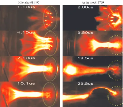
1.2 Images of hydrogen jet and argon jet. . . 13

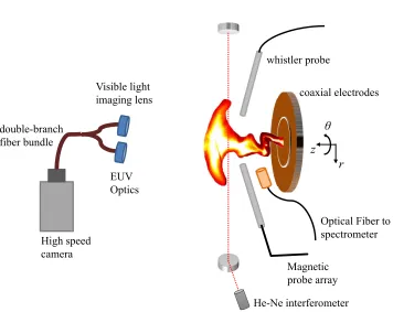
1.3 Overview of diagnostics . . . 16

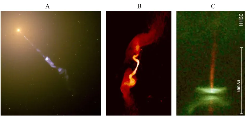
2.1 Examples of astrophysical jets observations . . . 22

2.2 Accretion disk - plasma gun analogy . . . 24

2.3 Evolution of energy in the simulation . . . 37

2.4 Current-Voltage profile in the experiment and simulation . . . 37

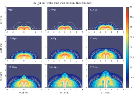
2.5 Time sequence of cross-sectional view of the plasma density and poloidal mag-netic field in a typical argon jet simulation . . . 41

2.6 Comparison of images of simulation jet and experimental jet . . . 42

2.7 Axial profiles of the simulation jet . . . 43

2.8 Cross-sectional view of the energy fluxes . . . 46

2.9 Radial profiles of the simulation jet . . . 47

2.10 Cross-sectional view of a set of plasma properties at t= 29.1µs . . . 49

2.11 Magnetic field structure of the experimental jet and the simulation jet . . . . 51

2.12 3D magnetic field structure of the simulation jet . . . 53

2.13 Alfv´en velocityvA and velocity to Alfv´en velocity ratio v/vA . . . 55

2.14 Jet velocity dependences in the simulation. . . 56

2.15 Bernoulli property of the jet . . . 58

2.16 Cross-sectional view of density distribution and poloidal flux contours of nine simulations with different conditions . . . 60

2.17 Simulation of a kinked hydrogen jet . . . 65

2.18 Simulation of two kinked hydrogen jets with larger poloidal currents . . . 66

(14)

3.2 Images of Rayleigh-Taylor instability in the kinked plasma jet. . . 73

3.3 Sketch of the plasma jet configuration in a lateral gravity . . . 75

3.4 largest eigenvalue of truncated matrixQpas a function of largest allowed mode number p . . . 88

3.5 Instability growth rate as a function of axial perturbation wave number/wave-length for the argon and hydrogen plasma jet . . . 93

3.6 Spectra of the fastest growing eigen-perturbation . . . 95

3.7 Pattern of fastest growing eigen-perturbation of argon and hydrogen jet . . . 97

3.8 yz cross-sectional view of the velocity and magnetic field of the fastest growing eigen-perturbation of argon jet solution . . . 98

3.9 xy cross-sectional view of the fastest growing eigen-perturbation of argon jet 99 3.10 Comprehensive solutions of the RT-CD coupled instability in the (α,Φ2) pa-rameter space . . . 101

3.11 Sketches of curved flux rope and lateral Rayleigh-Taylor instabilities . . . 104

3.12 SDO/AIA 171 EUV images of a CME in active region NOAA 11163, 02/24/2011106 4.1 Sketch of 2D X-point type Sweet-Parker reconnection . . . 121

4.2 3D magnetic field measurements of shot 17012 . . . 127

4.3 Composite images of EUV emission and visible light of the kinked argon jet undergoing Rayleigh-Taylor instability . . . 129

4.4 IV characteristics of shot 17012 . . . 129

4.5 3D magnetic field measurements of shot 16940 . . . 131

4.6 IV characteristics of shot 16940 . . . 132

4.7 Phases of the high-frequency magnetic fluctuations of shot 16940 . . . 133

4.8 Phases of the high-frequency magnetic fluctuations of shot 17012 . . . 134

4.9 Spectrograms of the 3D magnetic fluctuations of shot 17012 and 16940 . . . 135

4.10 10 MHz magnetic fluctuations from 29 to 30µs in shot 17012 exhibits circular polarization in hodogram . . . 137

4.11 Hodograms of 9 MHz and 12 MHz fluctuations in shot 17012 . . . 138

4.12 Polarization recognition of shot 16940, 17012, and 17014. . . 141

4.13 Direction of wavevectors of shot 17012 in time-frequency domain . . . 142

(15)

5.1 A simple equivalent circuit diagram of B-dot probe. . . 147

5.2 B-dot probe sensitivity as a function of frequency . . . 149

5.3 Unwanted capacitive coupling and RF ground loop in high-speed diagnostics 150 5.4 Sketches of shielded loop probe and dummy probe . . . 153

5.5 RF Ground loop diverting technique . . . 154

5.6 Effective schematics of the RF Ground loop for signal current and RF ground current . . . 155

5.7 Dummy probe test results with RF ground current diverting technique. . . . 156

5.8 Sketch of a pair of magnetic probes facing opposite direction . . . 159

5.9 Sketch of three pairs of dual differential probes enclosed in a quartz tube . . 160

5.10 Drawing of the vacuum assembly of the 3D magnetic probe . . . 161

5.11 Pictures of the shielded loop probe and the 3D magnetic probe . . . 161

5.12 Picture of the ferrite cores and shunt cables . . . 162

5.13 Output of the dual probes in Helmholtz coil. . . 164

5.14 Calibration of the high-speed 3D magnetic probe . . . 165

5.15 Magnetic fluctuations measured in shot 17012. . . 167

5.16 Output of each components of the dual probes in shot 17012 . . . 168

6.1 Circuit diagram of the transmitter and receiver of the high voltage probe . . 173

6.2 Three dimensional cross-section drawing of the transmitter without HV ca-pacitor C2. . . 174

6.3 Sketches of the lab-made cylindrical HV capacitor . . . 174

6.4 HV probe calibration result with C2= 60 pF . . . 179

6.5 Measurement results of shot 9950 using both the optically coupled HV probe and a Tektronix probe . . . 181

6.6 Optically coupled floating HV probes in use in the cross-flux-tube experiment, arched-loop experiment, and RF pre-ionized plasma jet experiment . . . 181

A.1 Peak transmission rate and FWHM of the tunable filter as a function of central wavelength. . . 188

(16)

A.4 Two-color imaging of the dual-species plasma jet using the VariSpec tunable filter . . . 190

(17)

List of Tables

(18)

Chapter 1

Background and Introduction

A plasma is an ionized gas containing freely moving ions and electrons and possibly neutral atoms. The charged particles in the plasma collide with other charged particles via Coulomb interaction. Motion of electrons and ions creates an electric current that further generates a magnetic field. On the other hand, an external magnetic field or self-generated magnetic field exerts a Lorentz force on the plasma when applied on the electric current. The coupling of electromagnetic forces and fluid effects leads to complex behaviors of the plasma.

The majority of the observable matter in the universe is in the plasma state, including stars, planetary nebulae, interstellar media, solar corona, solar wind, magnetosphere, etc. Man-made terrestrial plasmas are found in controllable fusion experiments and other plasma research experiments, plasma display, semi-conductor processing/manufacturing, and so on. Studying plasma is crucially important, not only for improving its existing usages in civilian applications, but also for solving human beings’ long-term sustainable energy problem, and for understanding the behaviors of the most abundant state of baryonic matter of our universe.

1.1 Magnetohydrodynamic theory

(19)

conductive fluid. The Eulerian form of the MHD equations in SI units are

continuity equation ∂ρ_∂t +∇ ·(ρv) = 0 (1.1) equation of motion ρ ∂_∂tv+v· ∇v=J×B− ∇P (1.2)

Ohm’s law E+v×B=ηJ (1.3)

Faraday’s law ∇ ×E=−∂_∂tB (1.4)

Ampere’s law ∇ ×B=µ0J (1.5)

energy equation _dtd

P ργ

= 0, (1.6)

where ρ is the plasma density, v is the bulk plasma velocity (velocity of center of mass of electrons and ions),P is the plasma pressure,E,B, andJare respectively the electric field, magnetic field, and current density vectors, η is the plasma resistivity, andγ = 5/3 is the adiabatic index for sufficiently collisional plasma.

The continuity equations, equation of motion, and energy equation are similar to those in hydrodynamics except that the equation of motion contains the Lorentz force. Ampere’s law is same as in the Maxwell’s equations in the non-relativistic limit.

Plasma that can be described by MHD equations must satisfy the following conditions:

• The plasma is charge-neutral. A charged particle in the plasma attracts oppositely

charged particles surround it like a charge shield. It can be shown that the charge-neutrality is true when the characteristic lengths of the plasma dynamics are much longer than Debye length λD =

q

0κBT

nq2 , where nis the particle number density and

q is the particle charge [e.g., see § 1.6 in Ref.5].

• The plasma is sufficiently collisional so that the particle distribution is Maxwellian

and the plasma can be treated as a single fluid. This is true for plasma dynamics that are much slower than the particle collision rate.

• The plasma phenomenon is nonrelativistic, so no relativistic effect shows up in the

MHD theory. For example, the pre-Maxwell version of Ampere’s law is used in MHD, which does not include the displacement current µ00∂_∂tE 1. We assume lchar and

1_{In fact, relativistic MHD equations are often used for many astrophysical situations, such as active}

(20)

tchar as respectively the characteristic length scale and time scale for a given plasma

phenomenon. Faraday’s law (Eq. 1.4) then givesE/lchar ∼B/tchar. The ratio of the

displacement current to the left-hand side of Eq. 1.5is then

|µ00∂_∂tE|

|∇ ×B| ∼

E/tchar

c2_B/l

char

∼ (lchar/tchar)

2

c2 ,

where we have used c = (µ00)−1/2. Therefore, the displacement current term is ignorable for non-relativistic phenomena havinglchar/tchar c.

• The characteristic time scale for a given plasma dynamics is much longer than the electron and ion cyclotron period 1/ωcσ =mσ/(eB) where σ =eor i. Equation1.2

shows that when the Lorentz force dominates the plasma dynamics there is J ∼ ωρU/B. Here ω is the characteristic frequency of the dynamics. Hence J/(ne) ∼ ωmiU/(eB) =ωU/ωciU ifω ωci. Therefore the differential velocity of electrons

and ions are much slower than the plasma bulk velocity. Equivalently speaking, the electron and ion motions are well coupled. This condition also leads to the fact that the Hall term in the electron equation of motion can be ignored to give the MHD Ohm’s law (see§ 4.1.2for details).

• The pressure and density gradients are parallel, so there is no thermoelectric effect

(also see §4.1.2).

(21)

1.1.1 Lorentz force and force-free configuration

Substitute Ampere’s law into the Lorentz force to obtain

J×B = 1

µ0

(∇ ×B)×B

= 1

µ0

B· ∇B− ∇

B2

2µ0

, (1.7)

where we have used the vector calculus identity ∇(C·D) = (C· ∇)D+ (D· ∇)C+C×

(∇ ×D) +D×(∇ ×C). WriteB=BBˆ and ∇B=∇(BBˆ) = (∇B) ˆB+B(∇Bˆ). Therefore

J×B = 1

µ0

B· ∇B− ∇

B2

2µ0

= B

2

µ0 ˆ

B· ∇Bˆ+ ˆB·

∇B

2

2µ0

ˆ

B− ∇

B2

2µ0

= B

2

µ0 ˆ

B· ∇Bˆ− ∇⊥

B2

2µ0

, (1.8)

where ∇⊥ is the gradient perpendicular to the magnetic field direction. It can be shown

that ˆB· ∇Bˆ = −R/Rˆ , where 1/Ris the local curvature of the field line and ˆR goes from the center of curvature to the field line, and hence the first term describes a force that tries to straighten out the curved magnetic field line. This tension-like component B_µ2

0 ˆ

B· ∇Bˆ is called the pinch force. The other pressure-like component of the Lorentz force∇⊥

B2 2µ0

is called the hoop force. Both components are perpendicular to the magnetic field line.

Force-free configuration is an arrangement of plasma that satisfies

∇ ×B=αB, (1.9)

where α is a scalar that might be spatially dependent. According to Ampere’s law, the force-free configuration has J= _µ1

0∇ ×B =

α

µ0BkB soJ×B = 0. Therefore no Lorentz force acts on the plasma in the force-free configuration.

Equation1.9indicates that a force-free configuration must be three-dimensional because the curl of a two-dimensionalB has component perpendicular to B.

Take the divergence of Eq. 1.9so the left hand side becomes zero. There is

(22)

ThereforeB⊥ ∇α, soα remains constant along magnetic field lines.

1.1.2 Ideal MHD magnetic flux frozen-in condition

Ohm’s law can be interpreted in two different aspects. One is to consider the traditional Ohm’s law in the plasma frame

E0 =ηJ0 (1.11)

and then switch to the lab frame using Lorentz transform in the low-speed limit

E0 = E+v×B (1.12)

J0 = J. (1.13)

Another aspect is to consider the electron equation of motion in two-fluid theory. After dropping the electron inertia term, the Hall term, and the pressure term, the electron equation of motion is reduced to Eq.1.3. A detailed discussion will be given in§ 4.1.2.

In thermal equilibrium, Fokker-Planck theory shows that the resistivity of a fully ionized plasma is [e.g., see §13.3 in Ref.5]

η= πZe

2_m1/2

e ln Λ

(4π)2₍_κ

BT)3/2

= 1.03×10−4Zln Λ

Te3/2

Ohm·m, (1.14)

whereZ is the ionization of ions, me is the electron mass,0 is the vacuum electric permit-tivity, ln Λ is the Coulomb logarithm and is usually taken to be 102, κB is the Boltzmann

constant, T is the plasm temperature in Kelvin, and Te is the plasma temperature in eV.

Equation 1.14 is called Spitzer resistivity [105]. It is seen that η ∝ T−3/2, meaning that higher temperature plasma has lower resistivity. This is because free electrons and ions with larger kinetic energy are less vulnerable to Coulomb interaction (collision) with other charged particles. Most astrophysical plasmas and many experimental plasmas have very high temperature and so very low resistivity.

2_{The parameter Λ is defined as Λ =}_λ

D/bπ/2, whereλD is the Debye length previously defined in§1.1, and bπ/2 =Ze2/(4π0mev02) is the impact parameter of 90◦-angle collisions of a Ze charged ion seen by

electrons with velocityv0. It can be shown that Λ = 6πnλ3D, wherenis the plasma particle number density. Therefore, Λ is a measure of number of particles in a sphere having a radius equal to the Debye length. Dependent on density and temperature, Λ can take value ranged from 102 _{to 10}11 _{in different plasmas.}

(23)

Ideal MHD theory takes the zero resistivity limitη = 0 so an ideal MHD plasma behaves like a superconductor. One of the most important properties of ideal MHD is that the magnetic flux is “frozen-in” to the plasma frame. To see this, we substitute Ampere’s law and the resistive Ohm’s law into Faraday’s law and obtain the MHD induction equation

∂B

∂t =∇ ×(v×B) + η µ0

∇2_B_. _(1.15)

Therefore, changes in magnetic field are caused by plasma motion and resistive diffusion. In ideal MHD there is no magnetic diffusion, so

∂B

∂t =∇ ×(v×B). (1.16)

Consider a surface S(t) in the plasma that moves together with the plasma. The total magnetic flux through the surface is

Ψ(t) =

Z

S(t)

B(x, t)·ds, (1.17)

wheredsis the elementary surface area vector perpendicular to the surface. Therefore, the changing rate of Ψ is

dΨ(t)

d = δtlim→0

R

S(t+δt)B(x, t+δt)·ds−

R

S(t)B(x, t)·ds

δt

= lim

δt→0

R

S(t+δt)

B(x, t) +δt∂B_∂t(x,t)

·ds−R

S(t)B(x, t)·ds

δt

= lim

δt→0

R

S(t+δt)B(x, t)·ds−

R

S(t)B(x, t)·ds

δt +

Z

S(t)

∂B(x, t)

∂t ·ds. (1.18)

(24)

written asds=vδt×dl. The first term in Eq.1.18 becomes

lim

δt→0

R

S(t+δt)B(x, t)·ds−

R

S(t)B(x, t)·ds

δt

= lim

δt→0

H

CB(x, t)·(vδt×dl)

δt

=

I

C

B·(v×dl)

= −

I

C

(v×B)·dl

= −

Z

S

∇ ×(v×B)·ds, (1.19)

whereCis the boundary ofS, and we have used the Stoke’s theorem to convert the boundary integration to a surface integration. Substitute this equation back to Eq.1.18 and get

dΨ(t)

d =

Z

S

∂B

∂t +∇ ×(v×B)

·ds= 0. (1.20)

Therefore, the magnetic flux enclosed by a closed material line is constant. It is usually stated (though not very rigorously) that the magnetic field line is “frozen-in” the plasma.

1.1.3 Dimensionless nature of ideal MHD

Ideal MHD has a very important property that it does not have any intrinsic scale. Equa-tions1.1-1.6are all written with dimensional variables. We define three nominal quantities: lengthL, magnetic field B0 and plasma density ρ0. Then we define several nominal quan-tities dependent on L, B0, and ρ0, which are velocity vA = B0/

√

µ0ρ0, time t0 = L/vA

and pressure P0 = B20/µ0 = ρ0v2A. After normalizing to these nominal quantities, the

dimensionless version of the MHD equations are

∂ρ˜

∂˜t + ˜∇ ·( ˜ρv˜) = 0 (1.21)

˜

ρ

∂v˜

∂˜t + ˜v·

˜

∇v˜

= ( ˜∇ ×B˜)×B˜ −∇˜P˜ (1.22)

∂B˜

∂˜t =

˜

∇ ×(˜v×B˜) + 1

S

˜

∇2_B_˜_, _(1.23)

where the tilde (˜) denotes the normalized physical quantities or operations. For example, ˜

(25)

Alfv´en wave propagating along the magnetic field lines. The Lundquist number is introduced as

S = µ0vAL

η . (1.24)

In the reduced MHD equations, the Lundquist numberSis the only scale-dependent param-eter. However,S is usually very large for most astrophysical and space plasma (S >1010) and laboratory plasma (S = 102−108), especially in fusion research experiments, because these plasma usually have very fast Alfv´en velocity and low resistivity, due to the strong magnetic field and high temperature. S 1 is equivalent to saying that the magnetic diffusion is ignorable compared to the magnetic convection in the dynamics. In this case the last term in the reduced MHD equations can be dropped. Therefore we obtain a set of dimensionless ideal MHD equations that are independent on the scale of the plasma.

One evidence of the scalability of ideal MHD is that astrophysical jets of vastly differ-ent scales and lifetimes are found to have very similar morphology, kinetic behavior, and magnetic field structure [30,45]. Arched flux rope structures that are found in solar corona can also be created in the lab experiment [107]. These facts indicate that the underlying physics of these plasma phenomena are described by ideal MHD.

The dimensionless nature of ideal MHD suggests that plasma dynamics of very large scales, such as astrophysical plasma, can be studied at a much smaller scale, such as in a terrestrial experiment, as long as the ideal MHD conditions are satisfied. A terrestrial experiment has several advantages over passive astrophysical observation, including the possibility of adjusting plasma parameters (i.e., active experiment) and in-situ diagnostics. Compared to numerical simulation, lab experiment includes real plasma effects. In the past decade there have been a rapidly increasing number of studies of using laboratory experi-ments to study astrophysics. In 2012, a new division, Division of Laboratory Astrophysics Division (LAD), was established in American Astronomical Society (AAS). “Laboratory astrophysics” has become an important branch in the modern astrophysical research.

(26)

1.1.4 Magnetic helicity and Taylor state

Magnetic helicity is an important concept of MHD plasma, and is defined as

K =

Z

V

A·Bd3r, (1.25)

whereA is the vector potential of the magnetic field and the integration is performed over the entire volume V of the plasma. A is undefined with respect to a gauge, i.e., A+∇f

gives the same magnetic field B as A with f being an arbitrary analytic scalar function. However,K turns out to be gauge invariant as long as no magnetic field line penetrates the surfaceS enclosing the volumeV [5].

Magnetic helicity is a topological measure of number of linkages of magnetic flux tubes with each other and number of twists of magnetic field. Topologically the linkage and twist are the same concept.

Denote φ as the electrostatic potential. Using Faraday’s law andE =−∇φ−∂tA, we

have

∂

∂t(A·B) = ∂A

∂t ·B+A· ∂B

∂t

= −(E+∇φ)·B−A·(∇ ×E)

= −E·B− ∇ ·(φB)− ∇ ·(E×A)−E·(∇ ×A)

= −2E·B− ∇ ·(φB+E×A). (1.26)

MHD Ohm’s law Eq.1.3 gives

E·B= (ηJ−U×B)·B=ηJ·B. (1.27)

Substitute this equation to Eq. 1.26and obtain

∂

∂t(A·B) +∇ ·(φB+E×A) + 2ηJ·B= 0. (1.28)

Integrate this equation over the entire volumeV and apply Gauss’s theorem to have

dK dt +

Z

S

ds·(φB+E×A) =−2

Z

V

(27)

For ideal MHD plasma the right-hand side of this equation is zero. Furthermore, if the ideal plasma is bounded by a conducting wall so that near the wall the magnetic field only has a tangential component and the electric field only has a normal component, the surface integral in the above equation then vanishes. Therefore, the magnetic helicity K is a conserved quantity in ideal MHD.

If the plasma is driven by a magnetized electrode system that has both electrostatic potential and magnetic field with normal component, the second integration is finite. More-over, the definition of absolute helicity in Eq.1.26is gauge-dependent. However, the relative helicity

Krel=

Z

V

(A·B−Avac·Bvac)d3r (1.30)

remains gauge invariant. It can be shown that the conservation law for the relative helicity is

dKrel

dt +

Z

∂V

(2VB)·ds=−2

Z

V

ηJ·Bd3r, (1.31)

where ∂V is surface of the electrodes [3, 61]. Therefore, helicity can be injected into a plasma by maintaining an electrostatic potential across two electrodes and having external magnetic field threading into the plasma.

Without external helicity injection, the magnetic helicity of an ideal MHD plasma is conserved. Woltjer-Taylor relaxation is a process where a plasma relaxes to a final state with minimum magnetic energy WB =

R

V B2 2µ0d

3_r _{while conserving the magnetic helicity.}

Variational method shows that for a zero-pressure plasma the minimum-energy state satisfies

∇ ×B=λB, (1.32)

where λ is a spatially uniform constant [121]. Magnetic reconnection dissipates magnetic energy but conserves helicity and therefore provides a mechanism for this relaxation [114]. The final state is called the Taylor state. Comparing with Eq.1.9it is seen that the Taylor state is a special force-free state.

(28)

greatly simpler facility. Meanwhile, the Spheromak is not susceptible to many instabilities that exist in Tokamak because of the different confinement concept.

1.2 Overview of Caltech plasma jet experiment

1.2.1 Experiment setup and jet dynamics

The Caltech experimental plasma jet is generated using a planar magnetized coaxial plasma gun mounted at one end of a 1.48 m diameter, 1.58 m long cylindrical vacuum chamber (sketch in Fig. 1.1). The coaxial gun is similar to those used for creating the Spheromak [34]. We define the central axis perpendicular to the electrodes as the z axis of a cylindrical coordinate system. The electrode plane is defined as z= 0. The radial and axial directions are called the “poloidal” direction and the azimuthal direction θ is called the “toroidal” direction. The vacuum pressure is ∼ 10−7 torr, corresponding to a background particle density of 3×1015 m−3 at room temperature. The plasma gun has a 19.1 cm diameter disk-shaped cathode and a co-planar annulus-shaped anode with inner diameter d= 20.3 cm and outer diameter D = 51 cm. At time t =−10 ms, a circular solenoid coil behind the cathode electrode generates a dipole-like poloidal background magnetic field for ∼ 20 ms, referred to as the bias field. The total poloidal field flux is about 1.5 mWb. Att=−1 ms to −5 ms, neutral gas is puffed into the vacuum chamber through eight evenly spaced holes at r = 5 cm on the cathode and eight holes at r = 18 cm on the anode at the same azimuthal angles. At t = 0, a 120 µF 5 kV high voltage capacitor is switched across the electrodes. This breaks down the neutral gas into eight arched plasma loops spanning from the anode to the cathode following the bias poloidal field lines, a geometry analogous to “spider legs”. At 0.6 µs after breakdown, a 4 kV pulse forming network (PFN) supplies additional energy to the plasma and maintains a total poloidal current at 60−80 kA for

≈40 µs. A typical current and voltage measurement is given in Fig. 2.4.

(29)

vacuum chamber

vacuum magnetic field

gas puff

bias coil

cathode

-5 kV C

Figure 1.1: Left: 3D cross-sectional view of the vacuum chamber and the coplanar coaxial plasma gun. Right: sketch of the plasma gun and the cylindrical coordinate. The central thick plane is the cathode. The sketch is not to scale.

mutually attract each other by the Lorentz force and merge into a single collimated plasma tube along the z axis. A ten-fold density amplification in the jet due to collimation is observed by Stark broadening and interferometer measurements; these show the typical density of the collimated jet is 1022−1023 m−3 [63,126,127]. The poloidal magnetic field strength in the plasma is also amplified from<0.05 T to∼0.2 T, indicating that the field is frozen into the plasma and is collimated together with the plasma. This amplification of the magnetic field strength has also been observed spectroscopically [102]. The thermal pressure and axial magnetic field pressure B_z2/(2µ0) increase until they balance the radial Lorentz force and lead to a nearly constant jet radius of 2−5 cm (Fig. 1.2) and a toroidal magnetic fieldBθ∼0.1−0.5 T (see experimental measurements in Fig. 2.11). This radial

equilibrium is gradually established from small to large z, resulting in an MHD pumping mechanism that accelerates the plasma towards the +z direction to form a jet. The typical jet velocity is 10−20 km s−1 for argon, 30−40 km s−1 for nitrogen, and∼50 km s−1 for hydrogen [63].

(30)

H jet shot#11497 Ar jet shot#13769

Figure 1.2: False color images showing the formation of a hydrogen plasma jet (left, shot 11497) and an argon plasma jet (right, shot 13769). The hydrogen shot only used the 120

(31)

the inductance of the plasma. In the plasma jet case, Ψ is the total toroidal flux. During the kink instability Ψ remains quasi-constant. Hence the plasma changes its shape from a straight column to a spiral solenoid to have a larger inductance and so relaxes to a lower energy state. A detailed theory of kink instability will be given in§ 3.5.1, as a special case of a Rayleigh-Taylor-Current-Driven coupled instability. Kink instability is a fundamental current-driven MHD instability that occurs in many other current-driven systems, such as Tokamak, Z-pinch plasma, solar flux ropes, and astrophysical jets.

When the kink grows exponentially fast and accelerates the plasma laterally away from the central axis, an effective gravitational force due to the acceleration is experienced by the plasma jet. At the inner boundary of the kinked jet, where this effective gravity points from the displaced jet (dense plasma) to thezaxis (zero-density vacuum), a Rayleigh-Taylor instability occurs [80]. The Rayleigh-Taylor instability eventually leads to a fast magnetic reconnection and destroys the jet structure. In Chapter 3 we will present an MHD theory of the Rayleigh-Taylor instability.

The jet life-time is∼10µs for hydrogen, 20−30µs for nitrogen, and 30−40µs for argon. Because heating is not important during this short, transient lifetime, the plasma remains at a relatively low temperature,Te∼2 eV, inferred from spectroscopic measurements [126].

Under typical experiment plasma conditions, the temperature relaxation time between elec-trons and ions is about 100 ns, less than 1% of the jet life time. Therefore, Ti ≈ Te ∼ 2

eV. At this temperature, the plasma is essentially 100% singly ionized according to the Saha-Boltzmann theory, which is also confirmed by spectroscopic measurements [49,126]. Figure 1.2 shows how the plasma is initially generated as eight arched loops, which then merge into one collimated jet. The jet then undergoes a kink instability when its length exceeds ∼30−40 cm and the Kruskal-Shafranov kink threshold is satisfied [49, 50]. For the current experiment configuration, the radius-length ratio of the jet in the final stage is about 1 : 10.

For a typical experimental plasma with ne= 1022m−3,Te =Ti = 2 eV,B = 0.2 T and

ion massµ≡mi/mH, the Debye length λD ≈10−7 m, the ion gyroradius ri ≈0.7

√

µmm,

and the ion skin depthdi≈2

√

(32)

and magnetic Reynolds numbersS ∼Rm&102×(L/0.3 m)/

√

µare both much greater than one withL∼0.3 m being the length of the jet. Therefore, ideal MHD theory can describe jet global dynamics, such as collimation, acceleration, and kinking [49,50,61,63,126,127], and magnetic field diffusion is negligible during the jet dynamics. The kinked jet image in Fig.1.2shows that the magnetic field is frozen into the plasma, consistent with ideal MHD theory. Therefore, the collimation of the bright plasma shown in Fig.1.2also demonstrates the collimation of the magnetic field. The secondary Rayleigh-Taylor instability, on the other hand, involves small-scale dynamics that are smaller than can be described by MHD theory [80].

1.2.2 Diagnostics and other apparatus

The transient experimental plasma jet varies from shot to shot, especially after the jet undergoes the kink instability. Therefore, measurements obtained by averaging over a large number of repeated single shots, which are commonly seen in other laboratory experiments, are not applicable in our experiment. Instead, high-speed diagnostics capable of resolving microsecond-scale plasma dynamics are required.

Diagnostic instrumentation used in the plasma jet experiment includes a high-speed visible-light IMACON 200 camera, a 30−60 eV band extreme ultra-violet (EUV) optical system [17], a 12-channel spectroscopic system [126], a He-Ne interferometer perpendicular to the jet [62], a 20-channel 3D magnetic field probe array (MPA) along the r direction with adjustable zand ∼1 µs response time [95], a whistler probe with excellent capacitive rejection and noise shielding (see Chapter 5), a Rogowski coil, and a Tektronix P6015A high-voltage probe. Figure.1.3 gives a sketch of the system.

The data acquisition (DAQ) system contains 12 eight-channel Struck Innovative Systeme SIS3300 data acquisition boards. Each channel has a ±0.5 V dynamic measurement range with 12-bit resolution and a sampling frequency of 100 MHz. Therefore, the digitization resolution of the DAQ system is 1/212= 0.244 mV.

The lab also owns a collection of optical bandpass filters and a VIS-7-35 VariSpec liquid crystal tunable filter. These filters when mounted in front of the IMACON200 camera can turn the camera into a 2D fast framing spectroscopic system.

(33)

r z

θ whistler probe

coaxial electrodes

Optical Fiber to spectrometer EUV

Optics Visible light imaging lens

High speed camera double-branch fiber bundle

Magnetic probe array He-Ne interferometer

Figure 1.3: An overview of some diagnostics in the plasma jet experiment. Not to scale.

Romero Talam´as [113]. In this section we will provide brief reviews of the fast framing IMACON 200 camera, the EUV optics built by Kil-Byoung Chai, and the VariSpec tunable filter. In AppendixAwe give a detailed description and some interesting applications using the tunable filter.

1.2.2.1 High-speed IMACON 200 camera

The IMACON 200 camera is an ultra-high-speed camera manufactured by DRS Technolo-gies. The IMACON camera contains an eight-way beam splitter system and seven functional monochrome 1360×1024-pixel 10-bit CCDs. Each of the CCDs records two images to give a movie of 14 frames in one experiment. The minimal inter-frame time between different CCDs is 5 ns and the waiting time between two frames of a single CCD is 200 ns. The IMACON 200 camera is sensitive to visible band and near-infrared band.

1.2.2.2 EUV optical system

(34)

nm Al film. The EUV optics converts EUV photons ranging from 30 eV to 60 eV (20−40 nm) to visible-light photons at an average converting efficiency of 5×10−4. Detailed infor-mation about the EUV optics is described in Ref. [17]. The EUV optical system is mounted inside the vacuum chamber with the phosphor screen facing a window. The IMACON 200 camera is focused on the phosphor screen through the window and records the visible im-ages converted from the EUV imim-ages. Another configuration is to use a double-branch fiber bundle to convey both the visible and EUV images simultaneously to the IMACON 200 camera, as shown in Fig.1.3.

1.2.2.3 VariSpec liquid crystal tunable filter

The VariSpec liquid crystal tunable filter is an optical filter with transmitting wavelength electrically controllable from 400 nm to 720 nm. It is claimed that the tunable filter has an integral hot mirror that can reflect infrared photons because the thermal energy carried by the infrared photons can affect performance of the filter or even cause damages. However, we found that the filter can still transmit a significant amount of near-infrared photons that can be recorded by the IMACON 200 camera. Therefore, an external hot mirror is mounted in front of the tunable filter. In Appendix A we provide a detailed description of the tunable filter and show a two-color imaging of the plasma jet experiment using the tunable filter.

1.3 Overview of this thesis

In Chapter 1 we have presented some brief introduction to plasma physics, MHD theory, and the Caltech plasma jet experiment. A more detailed introduction regarding specific topics will be given individually in each chapter.

(35)

comparison between the experiment and simulation give a comprehensive description of the jet collimation and acceleration processes. We study numerically the magnetic to kinetic energy conversion and obtain quantitative agreement between the simulation results and the experiment.

As shown in § 1.2.1, the plasma jet undergoes a global kink instability and then a secondary local Rayleigh-Taylor instability due to lateral acceleration of the kink instability. This Rayleigh-Taylor instability is very interesting because it occurs on a cylindrical surface of an MHD-collimated plasma tube and the direction of gravity is not always perpendicular to the interface. We found that the conventional hydrodynamic and magnetic Rayleigh-Taylor theories, which only consider 2D planar interface, give incorrect results when applied to our case. In Chapter 3 we use linear stability analysis to develop an MHD theory of the Rayleigh-Taylor instability on the cylindrical surface of a plasma flux rope in the presence of a lateral external gravity. The Rayleigh-Taylor instability is found to couple to the classic current-driven instability, resulting in a new type of hybrid instability. The coupled instability, produced by combination of helical magnetic field, curvature of the cylindrical geometry, and lateral gravity, is fundamentally different from the classic magnetic Rayleigh-Taylor instability occurring at a two-dimensional planar interface. The theory gives instability wavelengths and growth rates that match with experiments having several different configurations. We also show that this hybrid instability theory can be applied to many situations in solar physics.

Chapter 3solves the Rayleigh-Taylor instability in the early phase when the linear sta-bility analysis is still valid. In the experiment, however, this instasta-bility quickly evolves to a nonlinear phase and eventually leads to the failure of MHD. The Rayleigh-Taylor instability compresses and pinches the plasma jet to a scale smaller than the ion skin depth and then triggers a fast magnetic reconnection. In Chapter4we present measurements of high-speed magnetic fluctuations at the time of the reconnection and show that these fluctuations contain broadband right-hand circularly polarized whistler waves associated with the fast reconnection. With the specially designed high-speed 3D magnetic probe (Chapter 5), we are able to resolve the circular polarization of the whistler waves spontaneously generated in the fast magnetic reconnection.

(36)

The whistler probe consists of six shielded loop B-dot probes made of semi-rigid coaxial cables. We implement an RF ground current diverting technique that was first used by Perkins & Bellan (2011) [89]. The whistler probe has a 70 dB rejection to electrostatic interference, making it ideal for high-speed time-dependent magnetic field detection in an extremely noisy environment such as the Caltech plasma jet experiment.

(37)

Chapter 2

Three-Dimensional MHD

Numerical Simulation of Caltech

Plasma Jet Experiment

(38)

Primary part of this chapter was published by Xiang Zhai, Hui Li, Paul M. Bellan, and Shengtai Li, in Astrophysical Journal, Volume 791:40, 2014 [130]. This work is under the collaboration between Bellan group in Caltech and Li group in LANL.

2.1 Introduction

Magnetohydrodynamic (MHD) plasma jets exist in a wide variety of systems, from ter-restrial experiments to astrophysical objects, and have attracted substantial attention for decades. For example, energetic and usually relativistic jets are commonly observed, origi-nating from active galactic nuclei (AGNs), which are believed to be powered by supermassive black holes. AGN jets usually remain highly collimated for tens to hundreds of kiloparsecs from the host galaxy core [30]. It is generally accepted that AGN jets are powered by the central black hole accretion disk region. On a much smaller scale, stellar jets are believed to be an integral part of star formation, with an active accretion disk surrounding a young star [45]. See Fig. 2.1.

(39)

A B C

Figure 2.1: Panel A: Composite image of M87 AGN jet by Hubble Space Telescope. The yellow light are emissions from the host elliptical galaxy and the blue light are from syn-chrotron radiation by cyclotron motions of relativistic electrons. The length of the jet shown in the image is about 5000 light years or 5×1019 m. The jet is believed to be driven by a 3×109solar masses supermassive black hole and the surrounding accretion disk [56]. Credit: J. A. Biretta et al., Hubble Heritage Team (STScI /AURA), and NASA. Panel B: False color image of radio galaxy 3C31 (NGC 383) and its jet in 1.4 GHz radial band by VLA. The wiggled jet stretches to a distance of 300 kpc or 1022 m. Credit: Laing et al., NRAO. Panel C: HH30 protostellar jet and the accretion disk by Hubble (Burrows, STSci/ESA, WFPC2, NASA). The length of the jet is about 1000 AU or 1014 _m.

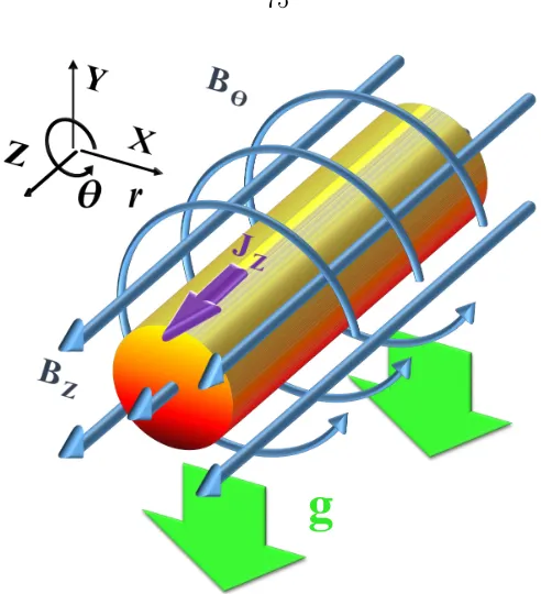
type of collimation mechanism, in which the axial currentJz and the associated azimuthal

magnetic field Bθ generate a radial Lorentz force and squeeze the jet plasma against the

pressure gradient at the central region of the jet.

The surprising similarities of astrophysical jets in morphology, kinetic behavior, and magnetic field configuration over vastly different scales have inspired many efforts to model these jets using ideal MHD theory. One important feature is that ideal MHD theory has no intrinsic scale (§ 1.1.3). Therefore, an ideal MHD model is highly scalable and capable of describing a range of systems having many orders of magnitude difference in size. Ideal MHD theory assumes that the Lundquist number, a dimensionless measurement of plasma conductivity, to be infinite. This leads to the well-known “frozen-in” condition, wherein magnetic flux is frozen into the plasma and moves together with the plasma [5] (see also

§1.1.2). Hence the evolution of plasma material and magnetic field configuration is unified

(40)

a magnetocentrifugal mechanism accelerates plasma along poloidal field lines threading the accretion disk; the plasma is then collimated by a toroidal dominant magnetic field at larger distance. Lynden-Bell (1996,2003) [74, 75] constructed an analytical magnetostatic MHD model where the upward flux of a dipole magnetic field is twisted relative to the downward flux. The height of the magnetically dominant cylindrical plasma grows in this configuration. The toroidal component of the twisted field is responsible for both collimation and propagation. The Lynden-Bell (1996,2003) [74,75] model and various following models, (typically numerical simulations with topologically similar magnetic field configurations; e.g., [68,69,73, 84, 122]), are called “magnetic tower” models. In these models, the large scale magnetic fields are often assumed to possess “closed” field lines with both footprints residing in the disk. Because plasma at different radii on the accretion disk and in the corona have different angular velocity, the poloidal magnetic field lines threading the disk will become twisted up [14, 69,73, 74,75, 100], giving rise to the twist/helicity or the toroidal component of the magnetic fields in the jet. Faraday rotation measurements to 3C 273 show a helical magnetic field structure and an increasing pitch angle between toroidal and poloidal component along the jet [128]. These results favor a magnetic structure suggested by magnetic tower models. Furthermore, it is (often implicitly) assumed that the mass loading onto these magnetic fields is small, so the communication by Alfv´en waves is often fast compared to plasma flows.

(41)

Black hole/protostar Magnetic field

Accretion disk

Differential rotation

Magnetic field -5kV

Accretion disk of astrophysical jet

Magnetized coaxial coplanar plasma gun

Poloidal field solenoid

Figure 2.2: Analogy of accretion disk system of astrophysical jet and magnetized coaxial coplanar plasma gun.

disk, it is seen that Er = vθBz, i.e., an equivalent radial electric field is created by θ

motion (rotation), and spatial integration of this electric field gives the voltage difference at different radii. Such a voltage difference is relatively easy to create in lab experiments by applying a voltage across a coaxial electrode pair (See § 2.2.3for the discussion on the helicity). Figure2.2shows the analogy of the magnetized coaxial coplanar plasma gun and the accretion disk system. Experimental jets are reproducible, parameterizable, and in-situ measurable. They automatically “calculate” the MHD equations and also “incorporate” non-ideal MHD plasma effects. Most importantly, the very fact that jets can be produced in the experiments strongly suggests there should be relatively simple unifying MHD concept characterizing AGN jets, stellar jets, and experimental jets [8].

(42)

collimated and straight and undergo a global kink instability when the jet length satisfies the classic Kruskal-Shafranov threshold [49, 50]. The Alfv´enic and supersonic jets cre-ated by the Caltech group have relatively low thermal to magnetic pressure ratio β ∼0.1 and large Lundquist number S ∼ 10−100. Other features including flux rope merging, magnetic reconnection, Rayleigh-Taylor instability, and jet-ambient gas interaction are also produced [49, 50, 80, 81, 126, 127]. See § 1.2 for a detailed introduction to the Caltech plasma jet experiments.

Observation, analytical modeling, numerical simulation and terrestrial experiments (lab-oratory astrophysics) are all crucial approaches for a better understanding of astrophysical jets. Compared to observation or analytical models, numerical simulation and terrestrial experiments share certain common features, such as the ability to deal with more complex structures and sophisticated behaviors, larger freedom in the parameter space compared to observation, and more resolution. However, cross-validation between numerical simulations and experiments has been very limited. Lab experiments can provide detailed validation for numerical models, while the numerical models can test the similarity between the terrestrial experimental jets and astrophysical jets.

(43)

is constant along the axial extent of the jet, is validated by analytical modeling, laboratory experiment, and the numerical simulation.

The chapter is organized as follows: In§2.2we describe the approach and configuration of our simulation, and show that the compact toroidal magnetic field injection method used in the simulation is equivalent to the energy and helicity injection through the electrodes used in the experiment. In § 2.3.1, we present the simulation results of a typical run, and compare these results with experimental measurements. In § 2.3.2, we perform multiple simulations with different toroidal injection rates and examine the jet velocity dependence on poloidal current. These results together with experimental measurements confirm the MHD Bernoulli equation and the magnetic to kinetic energy conversion in the MHD driven plasma jet. In§2.4we discuss the sensitivity of the simulation results to initial and injection conditions. In § 2.5 we present some preliminary results of the numerical investigation to kink instability. Summary and discussions are given in § 2.6.

2.2 Numerical MHD simulations

Discussion in this chapter is restricted to the global axisymmetric behaviors of the jet, such as collimation and acceleration. In this section, we prescribe appropriate initial and boundary conditions used to solve the ideal MHD equations numerically for the Caltech plasma jet experiment.

2.2.1 Normalization and equations

Number density, length and velocity are scaled to nominal reference values. In particular, density is normalized to n0 = 1019 m−3, lengths are normalized to R0 = 0.18 m (radial position of the outer gas feeding holes of the plasma gun in the experiment), and velocities are normalized to the ion sound speed Cs0 =

p

2kT /mi = 1.96 ×104

p

mH/mi m s−1

(with temperature 2 eV). All other quantities are normalized to reference values derived from these three nominal values and ion mass mi. Table 2.1 lists the derivation and the

(44)

Table 2.1: Normalization units for Experimental H/Ar Jet Simulation and AGN Jet Simu-lation

Quantity unit Quantity symbols H (µ= 1) Ar (µ= 40) AGN jet (µ= 1)

Length R0 0.18 m 0.18 m 15 kpc

Number density n0 1019_m−3 ₁₀19_m−3 ₃_×₁₀−3_cm−3

Speed Cs0 1.96×104m s−1 3.1×103m s−1 1.16×108cm s−1

Ion weight µ=mi/mH 1 40 1

Time t0=R0/Cs0 9.2µs 58.2µs 1.3×107yr

Mass density ρ0=n0mi/2 8.4×10−9kg m−3 3.3×10−7kg m−3 2.5×10−30 g cm−3

Pressure p0=ρ0Cs20 3.2 pa 3.2 pa 3.4×10−

11

erg cm−3

Temperature kBT=miCs20/2 2eV 2eV 7 keV

Energy E0=p0R3

0 0.0187 J 0.0187 J 3.4×1057 erg

Power P0=E0/t0 2.0×103_Watt _{321 Watt} ₂_.₆_×₁₀50_erg/yr

Magnetic field B0=√µ0p0 0.002 T 0.002 T 2×10−5_Gauss

Magnetic flux Ψ0=B0R20 0.0648 mWB 0.0648 mWB 4.4×10

40

G cm2

Current density J0=B0/(µ0R0) 8.871×103_{A m}−2 ₈_.₈₇₁_×₁₀3_{A m}−2 ₃_.₅_×₁₀−28_{A cm}−2

Current I0=J0R2

0 2.874×102A 2.874×102A 7.6×1017A

Voltage V0=P0/I0 7.07 V 1.118 V 1.1×1018V

The dimensionless ideal MHD equations, normalized to the quantities given in Table2.1, can be written as

∂ρ

∂t +∇ ·(ρv) = 0 (2.1)

∂(ρv)

∂t +∇ ·(ρvv+Pg ←→

I +PB

←→

I −BB) = 0 (2.2)

∂e

∂t +∇ ·[(e+Pg+PB)v−B(v·B)] = e˙inj (2.3) ∂B

∂t − ∇ ×(v×B) =

˙

Binj. (2.4)

The momentum equation and the energy equation have been written in the form of con-servation laws. We assume the same ion/electron temperature T =Ti =Te. The particle

number density n = 2ne = 2ni is used assuming singly-ionized plasma. The ionization

status is assumed to be time-independent. The equation of state for an ideal gas with adiabatic index γ = 5/3 is used. The gas pressurePg =nikBTi+nekBTe =nkBT is then

(45)

or magnetic energy density eB, is PB = eB = B2/(2µ0) and the total energy density is

e≡ρv2/2 +Pg/(γ −1) +PB. Compared to the MHD equations given in the introduction

Chapter, here we use the energy transportation equation2.3instead of the adiabatic energy equation1.6. They are equivalent mathematically but the energy transportation equation is easier to implement in the finite-volume numerical computation algorithm since it is written in the form of a conservation law.

An injection term ˙Binjis added to the induction equation. The associated dimensionless energy density injection is

˙

einj = ˙Binj·B, (2.5)

whereB is the magnetic field.

Simulations are performed in a 3D Cartesian coordinate system {x, y, z} using the 3D MHD code as part of the Los Alamos COMPutational Astrophysics Simulation Suite [LA-COMPASS, 70]. The solving domain is a cube [−4R0,4R0]3 = [−0.72 m,0.72 m]3, similar to the vacuum chamber size in the experiment. Each Cartesian axis is discretized into 800 uniformly spaced grids, giving a total of 5.12×108 grid points. The spatial resolution ∆x= 8R0/800 = 1.8 mm in the simulation is significantly greater than the Debye length, and is similar to the ion gyroradius and the ion skin depth of the plasma jet in the experiment. A typical run takes 5 to 24 hr on the Los Alamos National Lab Turquoise Network using 512 processors.

In contrast to the experiment where the jet exists only for positivez, the simulation has a mirrored plasma jet in the negativezdirection so as to have a bipolar system centered atz= 0 plane. The solving domain contains plasma only and has no plasma-electrode interaction region. Non-reflecting outflow boundary conditions are imposed at the boundaries (largex,

y orz). The MHD equations are solved in Cartesian coordinates so that no computational singularity exists at the origin.

2.2.2 Initial condition

2.2.2.1 Initial global poloidal magnetic field

(46)

two components separately. In Lynden-Bell (1996, 2003) [74,75], a poloidal field is assumed to be pre-existing, and the toroidal field is generated by twisting the upward flux relative to downward flux. During this process, the poloidal flux remains constant while toroidal field is enhanced with the increase of number of turns (helicity). These processes are realized equivalently in the lab experiment, where an initial dipole poloidal field is first generated by an external coil, and then helicity is increased by injecting poloidal current. In the simulation, an initial dipole poloidal magnetic field is similarly imposed, given by

Ψpol(r, z)≡2παp

r2

(l2₊_a2 0)3/2

e−l2, (2.6)

wherea0 ≡0.623R0 = 11.2 cm (R0= 0.18 m, see Table2.1) andl≡

√

r2₊_z2_{is the distance} from the origin. This configuration is topologically similar to the initial poloidal flux Ψpol=

r2e−l2 adopted by Li et al. (2006) [68]. By default, simulation equations/variables will be written in dimensionless form with reference units given in Table2.1. For example, Eq.2.6is the dimensionless version of Ψpol(r, z) = 2παpB0R20(r/R0)2/[(l/R0)2+ (a0/R0)2]3/2e−l

2_/R2 0, where B0 and R0 are given in Table 2.1. Compared to the ideal infinitesimal magnetic dipole flux Ψ∝r2/l3, Ψpol contains a constant factora0 to make the dipole source finite; it also has an exponential decay at large distance so that the initial field vanishes at the solving domain boundaries. At small r and z, Ψpol ∝r2 hence Bz is nearly constant. a0 is selected so that Ψpol(r = r1, z = 0) = Ψpol(r = r2, z = 0), where r1 = 0.278 ⇒ 5 cm and r2 = 1⇒ 18 cm corresponding to the radii of the inner and outer gas lines in the experiment. The dimensionless parameterαpquantifies the strength of the flux. The vector

potential can be selected to be A= (Ψpol/(2πr))ˆθ. The initial poloidal field is

Bpol =∇ ×A= 1

2π∇Ψpol× ∇θ (2.7)

⇒     

   

Br=

αpzre−l

2 (l2₊_a2

0)5/2

(3 + 2a2₀+ 2l2)

Bz=

αpe−l

2 (l2₊_a2

0)5/2

2(1−r2)(l2+a2₀)−3r2

, (2.8)

where ˆθ is the azimuthal unit vector and∇θ= ˆθ/r. The total poloidal flux is

(47)

where ro = 0.5667⇒ 10.20 cm is the position of the null of the initial poloidal field, i.e.,

Bz(ro,0) = 0. The first frame of Fig.2.5shows the flux contours of the initial poloidal field

in therz plane.

The toroidal current associated with the poloidal field is

Jθ=∂zBr−∂rBz =−αp

re−l2

(l2₊_a2 0)7/2

·g(l), (2.10)

where

g(l) = 4l6+ (8a₀2+ 2)l4+ 4a2₀(a2₀−2)l2−5a2₀(a2₀+ 3). (2.11)

Simple calculation shows thatl0= 0.9993≈1 is the only zero point ofg(l) andg(l)<0 for 0≤l < l0 and g(l)>0 for l > l0.

2.2.2.2 Initial mass distribution

In the experiment, plasma is initially created following the path of initial poloidal field lines (see Fig. 1.2 H jet at 1.1 µs and Ar jet at 2.0 µs), i.e., the plasma is distributed around the Ψpol(r, z) = Ψ0 surface. Here Ψpol(r, z) is the initial poloidal flux function (Eq. 2.6) and Ψ0 ≡Ψpol(r1,0) = Ψpol(r2,0) is the flux contour connecting the inner (r1 = 5 cm) and outer (r2 = 18 cm) gas feeding holes. A possible choice for the initial mass distribution function in the simulation isninit ∼exp[−δ(Ψpol(r, z)−Ψ0)2].

Note that this initial distribution has low plasma density on the axis. In the experiment, fast magnetic reconnection occurs as the eight arched loops merge into one. This allows the plasma and magnetic field to fill in the central region. The ideal MHD simulation, however, lacks the capability to simulate the fast magnetic reconnection, and hence cannot accurately describe the merging process. As a compromise, we start the simulation immediately after the merging process but before the collimation and propagation processes. We therefore choose a simple form topologically similar to the contour Ψpol(r, z) = Ψ0 but without the central hollow region, namely

ninit(r, z) = 1 +ninit,0·e−l 2

·e−δ[(r−1/2)2+z2−1/4]

2

. (2.12)

(48)

dense than the plasma jet. ninit,0 is the assumed initial plasma number density. The

e−δ[(r−1/2)2+z2−1/4]

2

term states that the plasma is initially distributed over a torus surface (r−1/2)2+z2 = 1/4, connectingr= 0 andr = 1 = 18 cm at mid plane. The torus surface is roughly parallel to the initial poloidal flux surface Ψpol(r, z) = Ψ0, but without the central hole. Thee−l2 term assures that the initial plasma is localized around the origin. Using this distribution, the central regionr'0 in the simulation is initially filled with dense plasma.

2.2.3 Helicity and energy injection

2.2.3.1 Compact injection near the z=0 plane

Toroidal magnetic flux is continuously injected into the simulation system, in order to replicate the energy and magnetic injection through the electrodes in the experiment. The helicity conservation equation in an ideal MHD plasma with volume V is

dKrel

dt =−

Z

∂V

(2VB)·dS= 2Ψpol·∂(IL)

∂t , (2.13)

whereKrel is the relative magnetic helicity,∂V is the boundary of the volume and the area

dS is normal to the boundary, V is the electrode voltage, I is the total current through the plasma, and L is the plasma self inductance across the electrodes [3, 9, 31, 61] (also see § 1.1.4). The electrode surface in the experiment is the effective∂V. When a poloidal magnetic field is present, Eq. 2.13 states that magnetic helicity injection can be realized either by maintaining a non-zero voltage across the electrodes, or by increasing the poloidal current/toroidal field in the plasma. In the experiment, these two methods are essentially equivalent. Meanwhile, magnetic energy is also injected into the plasma by ˙E=P =IV =

IdΨtor/dt, where Ψtor is the toroidal magnetic flux. Since neither electric field nor potential

is explicitly used in the simulation, we choose the second method to inject helicity. Thus we inject toroidal magnetic field into the system to increase the poloidal current and the magnetic helicity. The toroidal field injection term in Eq.2.4 is defined as

˙

(49)

whereγb(t) is the injection rate and

Btor =

f(Ψpol) 2πr e

−Az2 ˆ

θ= 1

2πf(Ψpol)e −Az2

∇θ (2.15)

is a pure toroidal field. The localization factorA is a large positive number so that toroidal field injection is localized near thez= 0 plane. f(Ψpol) is an analytical function of Ψpol and following the magnetic tower model used in Li et al. (2006) [68], we choosef(Ψpol) =αtΨpol so that

Btor=αtαp

r

(l2₊_a2 0)3/2

e−l2e−Az2 =αtαp

r

(r2₊_z2₊_a2 0)3/2

e−r2−(A+1)z2. (2.16)

The poloidal current associated with this toroidal field is

Jpol =∇ ×Btor = 1 2π∇

αtΨpole−Az 2

× ∇θ=αte−Az

2 Bpol+

αtΨpol

πr Aze

−Az2 ˆ

r, (2.17)

where∇ × ∇θ= 0 and Eq. 2.7are used.

At z = 0, Btor = αtΨpol/(2πr). Therefore the net poloidal current within radius r is

2πrBtor =αtΨpol. Using Eq.2.9, the total positive poloidal current associated withBtor is

Ipol= 2.488αtαp ⇒0.704αtαp kA. (2.18)

The localization factorA has no impact on the total poloidal current.

It is important to point out that the field injection term in the induction Eq. 2.4 is a compromise used to avoid having a plasma-electrode interaction boundary condition. Theoretically, Eq. 2.4 is not physically correct because of the injection term. However, because the localization factor A is a large positive number, the magnetic energy of Btor decreases rapidly withz. Therefore the “unphysical” region is very localized to the vicinity of the z = 0 plane. In particular, using A = 9, the total toroidal magnetic energy at the z = 0.307 ⇒ 5.5 cm plane is only 10% of the total planar magnetic energy at the

z = 0 plane. The toroidal magnetic flux within |z| < 0.307 contributes 87% of the total toroidal flux, although the volume is only 7.7% of the total simulation domain. We define

(50)

“jet region” where unphysical toroidal field injection does not occur. In the engine region, the toroidal magnetic field is directly added to the existing configuration by the modified induction equation (Eq. 2.4). The injection also adds magnetic helicity, poloidal current, and magnetic energy. In the jet region, on the other hand, this direct injection is negligible so the ideal MHD laws hold almost perfectly. The helicity, current, and energy enter the jet region with the plasma flow.

In the simulations presented here, we useA= 9. Although the choice of Ais somewhat arbitrary, in general, A needs to be sufficient large to localize the engine region to the vicinity of the z = 0 plane. This compact engine region serves as an effective plasma-electrode interface, and leaves most of the simulation domain described by the correct induction equations (i.e., no artificial injection). If a small A were used, injection would occur globally. There would then be a large amount of energy directly added to remote regions with low density plasma. A magnetized shock would then arise and dissipate injected energy. Using a largeA guarantees that the magnetic field is mostly frozen into the dense plasma. However, A should be not too large in our simulation, since otherwise numerical instability and error would occur because of excessive gradients.

The process of helicity/energy injection in the simulation is not exactly the same as in the experiments or the astrophysical case. In the experiment, a non-zero electric potential drop between the electrodes is responsible for the process. In AGN jet or stellar jet cases, the injection process could also be accompanied by electric potential drop in the radial direction as a result of interaction among the central object, wind, magnetic field, and the accretion disk dynamics, such as differential rotation of the disk and corona. However, the artificial injection of a purely toroidal field should produce mathematically equivalent magnetic structure. This injection is also consistent with the asymptotic X-winds solution by Shu et al. (1995) [103] and Shang et al. (2006) [98].

2.2.3.2 Jet collimation as a result of helicity/energy injection