PETRI NET BASED ALGORITHMIC APPROACH FOR
VECHICAL ROUTING PROBLEM
Sunita Kumawat
1, Pooja Yadav
2, Lajwanti
3, Naina Gupta
4,G.N.Purohit
51,2,3,4,
Department of Applied Mathematics, Amity University Haryana, Gurgaon, (India)
5Department of Applied Mathematics, Banasthali University Rajasthan, Rajasthan, (India)
ABSTRACT
In this paper, we consider the Vehical Routing Problem (VRP). Where VRP is modelled as a VRP-graph, in
which each edge is treated as a parallel combination of oppositely directed edges. We model VRP-graph as a
Petri Net-graph, where Petri Net- graph is an underlying graph of VRP-graph. Then solve VRP by defining
suitable binary operation on elements of columns in sign incidence matrix representation of Petri Net-graph. In
Petri Net-graph, we find a set of places which is both Siphon and Trap with minimum sum of capacities, whose
set of input transitions equals to the set of output transitions, and both of them are equal to the set of all
transitions in Petri Net. Then edges in VRP-graph corresponding to these places in Petri Net-graph will form a
shortest route for the seller to return the point of origin, after traversing all the cities exactly ones. For the
solution of VRP, we describe a new algorithm, based on siphon-trap and bounded-ness property of the Petri
Nets. 2000 Mathematics Subject Classification: 68R10, 90C35, 94C15.
Keywords: Travelling Seller’s Problem, Weighted Directed Graph, Spanning Cycle, Petri Net,
Siphon and Trap.
I. INTRODUCTION
The Vehical Routing Problem (VRP) is one of the most intensely studied problems in computational mathematics [5]. Mathematical problems related to the VRP were treated in the early nineteenth century by W.R Hamilton and British mathematician T. P. Kirkman. Although there are many algorithms given for the solution of VRP [6, 7, 8, 13, 14], yet no effective solution is known for the general case for the VRP. In this paper, we address the same problem with a different approach, using Petri Net model. Here we present a new algorithm to solving a VRP using the siphon-trap and bounded-ness property of the places in the One-one Petri Net model of given VRP-graph. For the VRP we find a set of places in Petri Net, which is both Siphon and Trap [1, 3], with minimum sum of capacities, having the property that set of input transitions equals to the set of output transitions, and both of them are equal to the set of all transitions given in the Net. Then edges in VRP-graph corresponding to these places form a shortest route for the seller.
272 | P a g e emphasized in the study of the Petri Nets. The most interesting connections between graph theory and Petri Nets have been brought out by T.Murata [9].
This paper is organized as follows: Section 2 provides the necessary preliminaries, Section 3 formulates the problem, Section 4 describes the algorithm for VRP with illustrative example and Section 5 briefly concludes this paper.
II. AN OVERVIEW OF PETRI NET APPROACH
This section of the paper provides the necessary preliminaries for the readers who are not familiar with Petri nets.
As Petri Nets are also called place-transition net (PT-Net), it is a particular kind of directed graphs together with an initial state called the initial marking. In general a Petri Net is an underlying graph of any directed graph, which is in essence a directed bipartite graph with two types of nodes called places and transitions. The arcs are either from places to transitions (output of places) or from transitions to places (input of places). In the Petri Net graph a place is denoted by a circle, a transition by a box or a bar and an arc by a directed line. A Petri Net is a PT-Net with tokens assigned to its places denoted by black dots, and the token distribution over its places is done initially by a marking function denoted by M0. A token is interpreted as a command given to a condition
(place) for the firing of an event (transition). An event can happen, when its all input conditions are fulfilled, See Fig.1
.
Fig.1
There are many subclasses of Petri Nets such as One-one Petri Nets, free choice Petri Nets, colored and stochastic Petri Nets etc. Here we introduce only One-one Petri Net, as it is an ordinary Petri Net such that each place P has exactly one input transition and one output transition having weight one on each edge, but we ignore these weights generally in the model representation of the Net PN. One-one Petri Net is also called as Marked Graph [4]. In our paper standard notation PN is treated as One-one Petri Net. More detailed and formal description of Petri Nets is given in [2, 9, 10, 15]. We include here some basic definitions, which are relevant to this paper.
Definition 2.1: A place-transition net (PT-Net) is a quadruplet PN = P, T, F, W, where P is the set of places, T is the set of transitions, such that P T and P T=, F (P x T) (T x P) is the set of arcs and W: F
{1, 2 ...} is the weight function. PN is said to be an ordinary PT-Net if and only if W: F {1}.
A marking is a function M0: P {0, 1, 2, ...},which distributesthe tokens to the places initially. Here M0 (p) is
the number of tokens in the place p at initial marking M0, it is a non- negative integer less then or equal to the
capacity of the place. Capacity of the place is defined as the capability of holding the maximum no. of tokens at any reachable marking M from M0. A marking M is said to reachable to M0 if there exist a firing sequence σ =
P, T, F, W without any specific initial marking is denoted by PN and Petri Net with the given initial marking is denoted by PN, M0. *x and x* are the set of input transitions (or places) and the set of output transitions (or
places) respectively, as x P (or T). Here | *x | and | x* | stands for number of the input transitions (or places) and the output transitions (or places) respectively. Thus a One-one Petri Net is an ordinary PT-Net such that p P: |*p|=|p*| =1, i.e., the number of the input transitions for p P equals to the number of the output transitions and both of them are equal to one.
For a PT-Net, a path is a sequence of nodes = x1, x2… xn where (xi, xi+1) F for i = 1, 2… n-1. is said to
be elementary if and only if it does not contain the same node more than once and
a cycle is a sequence of places p1 , p2 , …pn such that there exist t1, t2,…, tn T : p1, t1, p2, t2,…., pn , tn
forms an elementary path and (tn, p1) F.
Definition 2.2: For a PT-Net PN, M0, a place p is said to be k-bounded (or bounded by k) where k R+, if and
only if M0 (p) < k., denotes the capacity of the place in the Net. (PN, M0 is said to be k-bounded if and only if
every place is k-bounded.
Definition 2.3: A non-empty subset of places S is called a Siphon if *p p* pS denoted also *S S*; i.e., every transition having an output place in S has an input place in S. Likewise a non-empty subset of places Q is called a Trap if p* *p pQ denoted also Q* *Q; i.e., every transition having an input place in Q has an output place in Q.
III. PROBLEM FORMULATION: VEHICAL ROUTING PROBLEM (VRP)
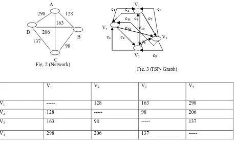
For a given network of cities and the cost of travel between each pair of them, the Vehical Routing Problem or VRP for short, is to find the shortest route for the seller, visiting to all of the cities exactly ones and returning to the starting point. In the standard version of VRP, the travel costs or distances are symmetric in the sense that travelling from city X to city Y costs just as much as travelling from Y to X. Any round-trip tour that goes through every city exactly once is a feasible tour with a given cost, if it is smaller than the other minimum cost tour.
3.1
Modelling VRP as a Graph (VRP-graph)
:
A pair G = {V, E}, where V= {v1,v2,v3,…,vn} is the set of vertices and E = {e1,e2,…,em} is the set of edges such
that each edge ei having some weights wiW, where W:E R +
is the weight function and wi =w(ei) is the
weight associated with edge ei . Further when the edges vi vj and vj vi are considered different then G={V,E} is
called a weighted directed graph. In weighted directed graph, a directed cycle is a closed sequence of directed edges without repetition of vertices except terminals and it said to be Spanning if it contains all the vertices of the graph. If any edge from the sequence is deleted then cycle becomes open. Thus solving a VRP amounts to finding a minimum weight spanning cycle.
274 | P a g e Distance between two cities in Fig.3 can be represented in terms of adjacency matrix as depicted below:
3.2
Modelling VRP-graph by Petri Nets:
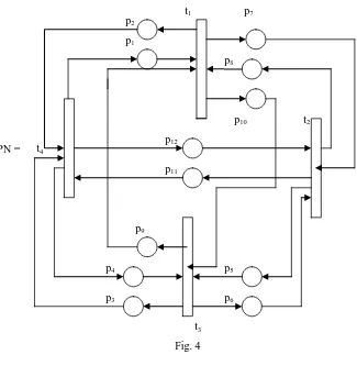
A Petri Net PN is modelled from VRP-graph given in Fig. 3 as follows: edges es are transformed into places ps
and vertices vk are transformed into transitions tk so that the place ps has an input from a transition ti, and an
output to a transition tj, if es is an directed edge vi vj in graph, then weights (distance between two cities) of es’s
are replaced by capacities ks of corresponding places ps and number of tokens for places ps‘s is the value of
k
s .Fig. 4 shows the One-one Petri Net model say PN, of the VRP-graph, having the set of transitions T= {t1 t2, t3,
t4} and the set of places is P = {p1, p2,…,p12 }corresponding to the set of vertices{v1,v2,v3,v4} and the set of edges
{e1,e2,…,e12} respectively in the given VRP-graph. For the sake of clarity, we observe that t1 is the input
transitions for the places p2, p7, p10 and the output transition for the places p1, p8, and p9. Similarly p1 is the input
place for the transition t1 and output place for the transitiont4. Using this same procedure, we find a set of the
places in Net which is both siphon and trap with minimum sum of capacities, whose set of the input transitions equals to the set of output transitions and both of them are equal to the set of all transitions in the Net PN.
V1 V2 V3 V4
V1 --- 128 163 298
V2 128 --- 98 206
V3 163 98 --- 137
V4 298 206 137 ---
TSP- Graph)
Fig.1
e1
V1
V3
V2
V4
e2 e8
e3
e7
e4
e5
e10
e9
e11
e12
e6
Fig. 3 ( A
D
B
C Fig. 2 (Network)
128
206 163 298
137
98
IV. DESCRIPTION OF ALGORITHM FOR TRAVELLING SELLER’S PROBLEM
As in above we model the VRP-graph as a Petri Net-graph. Now here we present an algorithm for solving the Travelling Seller’s Problem.For the description of the algorithm for VRP; we introduce some new notations as follows [16]:
In a Petri Net PN with n-transitions and m-places, the sign incidence matrix I = [aij] is the
n x m matrix, whose entries are defined as,
aij = + if place j is an output place of transition i.
aij = - if place j is an input place of transition i.
aij = ± if place j is both input and output places of transition i
(i.e., transition i and place j form a self loop) aij = 0 otherwise.
As an illustration, the Sign incidence matrix I of PN is:
p1 p2 p3 p4 p5 p6 p7 p8 p9 p10 p11 p12
t1 - + 0 0 0 0 + - - + 0 0
t2 0 0 0 0 + - - + 0 0 + -
t3 0 0 + - - + 0 0 + - 0 0
t1
t2
t4
t3
p2
p1
p7
p8
p10
p12
p11
p9
p4
p3
p5
p6
276 | P a g e
t4 + - - + 0 0 0 0 0 0 - +
Hare we introduce a commutative binary operation, denoted by on the set U= (0, +, - ,). defined as following:
+ - = ‘+’ entry is said to be neutralized by adding a ‘–‘entry to get a ‘±’ entry. a a = a aU
a = aU
0 a = a aU
For the VRP, we choose a subset of k places X = {p1, p2…pk} in sign incidence matrix I of PN, which is both
siphon and trap and also *X= X* = T, i.e., set of the input transitions of X is equals to the set of output transitions of X, and both of them equal to the set of all transition in T. This equality holds only if the addition under the operation , of the k column vectors say C1, C2, C3,…, Ck i.e., C1 C2 C3….. Ck contains only ±
entries everywhere, where Cj , j = 1, 2... k, denotes the column vector corresponding to the place pj in I.
Now let C1 C2 C3….. Ck will be a column vector denoted by γ = [γi] where γi denotes the i th element of the column vector γ, have as elements from set U. Then from the definition of I under the
operation, we interprets about γi as.
γi = 0 means no place in X is an input or output place of transition i.
γi = - means some place in X is an input place of transition i.
γi = + means some place in X is an output place of transition i.
γi = ± means some place in X is an input place as well as output place for
transition
i.
From the above it can be seen that every transition having an output place in X has an input place in X only if γi +, and likewise every transition having an input place in X has an output place in X only if γi-. So X is
both siphon and trap if and only if γ has either 0 or ± entries. And if γ has only ± entries everywhere, then the places corresponding to columns C1, C2, C3,…, Ck in C1 C2 C3….. Ck forms a set of places, which is both
siphon and trap, whose input transitions equals to the output transitions and both of them are equal to the set of all transitions T, with having some capacities. We select only those set of places X such that *X = X* = T, having minimum sum of capacities among all. Algorithm discussed below, gives us a siphon–trap set of places X with minimum sum of capacities, having the property *X = X* = T, whose corresponding edges in VRP-graph will form a shortest route for the seller, we follow for this [16].
ALGORITHM:
Input Sign incidence matrix I of order n x m.
Step 1 Select Cj, the first column in the sign incidence matrix I having ‘+’ entry whose corresponding place and
capacity is denoted as PLACEj and CAPACITYj
Set recursion level r to 1 Set Vjr = Cj
Set PLACEjr = PLACEj;
Set X =, W=, Sum =0 and K =.
Step 2 If Vjr has a ‘±’ entry at the i th
row then PLACEjr is a self loop with transition i, Go to Step 5.
Step 3 If Vjr has a ‘+’ entry in the kth row find a column Cs which contains a ‘–‘entry at kth row.
(i) If no such column Cs exists then go to Step 5.
(ii) If such Cs exists, add it to Vjr to obtain Vj(r+1) = Vjr Cs, containing a ‘±’ entry at kth row. Then
PLACEj(r+1) = PLACEjr PLACEs
CAPACITYj(r+1) = CAPACITYjr CAPACITYs
(iii) Repeat this step for all neutralizing columns Cs. This gives a new set of Vj(r+1)’s, PLACEj(r+1)‘s and
CAPACITYj(r+1)
Step 4 Increase r by 1, Repeat Step 3 until there are no ‘+’entries in each Vjr = C1 C2 C3….. Cjr.
Step 5 Any Vjr with all entries as ‘±’ represents both siphon and trap such that their input transitions equal to the
output transitions and both of them equal to the set of all transitions T. X = X PLACEjr
K= K CAPACITYjr
W=Sum + Sumw K, where Sumw K is the sum of the capacities in the set K Store it any other set and compare it to minimum weight set at each iteration
Step 6 Delete Cj
j = j + 1 Go to Step 1.
Output: Set X has places both siphon and trap such that their input transitions equal to the output transitions and both of them equal to the set of all transitions T with minimum sum of capacities. Whose corresponding edges set in VRP-graph, forms a shortest route for the seller.
As an illustration consider the graph in Fig 2.
Step 1 Select first column having ‘+’ entry. Here is C1, then
11
V
=
0
0 ; PLACE11 = {pl}; CAPACITY11 = {137}
Steps 2, 3 and 4, V11 has a ‘+’ entry at 4th row. The neutralizing columns are C2, C3 and C11.
V
12(1) =11
V
C2 =
0 0
0 0 =
0
0 ; PLACE12(1) = {pl , p2}; CAPACITY ) 1 (
12={137,137 }
V
12(2) =11
V
C3 =
0
0
0 0
=
0 ; PLACE(2)
12 = {pl, p3}; CAPACITY ) 2 (
278 | P a g e
V
12(3) =11
V
C11 = 0 0 0 0 = 0
; PLACE12(3) = {pl, p11}; CAPACITY ) 3 (
12 = {137,298}
) 2 ( 12
V
has ‘+’ entry at 3rd row. The neutralizing columns are C4, C5 and C10.
V
13(1) =V
12(2) C4 = 0 0 0 =
0 ; PLACE(1)
13 = {pl,p3, p4}; CAPACITY ) 1 (
13= {137,206,206}
V
13(2) =V
12(2) C5 = 0 0 0 =
; PLACE13(2) = {pl, p3, p5}; CAPACITY ) 2 (
13 = {137, 206,128}
V
13(3) =V
12(2) C10 = 0 0 0 =
0 ; PLACE13(3)= {pl, p3, p10}; CAPACITY ) 3 (
13 = {137, 206,98}
) 3 ( 12
V
has ‘+’ entry at 2nd row. The neutralizing column is C6, C7 and C12.
V
13(4) =V
12(3) C6 = 0 0 0 =
; PLACE13(4) = {pl, p11, p6}; CAPACITY ) 4 (
13 = {137,298,128}
V
13(5) =V
12(3) C7 = 0 0 0 = 0
; PLACE13(5) = {pl , p11, p7}; CAPACITY ) 5 (
13 = {137,298,163}
V
13(6) =V
12(3) C12 = 0 0 0 = 0
; PLACE13(6) = {pl, p11, p12}; CAPACITY ) 6 (
13 = {137,298,298}
) 1 ( 13
V
andV
13(6) has no ‘+’ entry , also all the entries are not ‘±’ only, but those sets which have all entries ‘±’ or ‘0’ are both siphon and trap ( as (1)12
V
,V
13(3)andV
13(5))) 2 ( 13
V
14(1) =V
13(2) C6 = 0 0 = ; PLACE14(1) = {pl, p3, p5, p6}; CAPACITY ) 1 (
14= {137,206,128,128}
V
14(2) =V
13(2) C7 = 0 0 =
; PLACE14(2) = {pl, p3, p5, p7}; CAPACITY ) 2 (
14 = {137,206,128,163}
V
14(3) =V
13(2) C12 = 0 0 =
; PLACE14(3) = {pl, p3, p5, p12}; CAPACITY ) 3 (
13 = {137,206,128,298}
) 4 ( 13
V
has ‘+’ entry at 3rd row. The neutralizing columns are C4, C5, and C10.
V
14(4) =V
13(4) C4 = 0 0 =
; PLACE14(4) = {pl, p6, p11, p4}; CAPACITY ) 4 (
14 = {137,298,128,206}
V
14(5) =V
13(4) C5 = 0 0 =
; PLACE14(5) = {pl, p6, p11, p5}; CAPACITY ) 5 (
14 = {137,298,128,128}
V
14(6) =V
13(4) C10 = 0 0 =
; PLACE14(6) = {pl, p6, p11, p10}; CAPACITY ) 6 (
14 = {137, 298, 128, 98}
) 1 ( 14
V
,V
14(3),V
14(4) andV
14(5) has no + entry.V
14(2),V
14(6) have allthe entries as ‘±’, Hence
PLACE14(2)and PLACE14(6) form both siphon and trap whose input transitions equal to the output transitions and both of equal to the set of all transitions.Step 5 the subsets of places, which are both siphon and trap, whose input transitions equal the output transitions and both of them equal to the set of all transitions are{pl, p3, p5, p7}and {pl,, p6, p11, p10}with capacities sum 634
and 661 as choosing column first C1.
Step 6 now delete C1 fromsign incidence matrix, choose next column and repeat all the steps again in similar
way, we get another different sets of places {p2, p4, p6, p8},{p2, p9, p5, p12}, {p3, p8, p10, p12} and{p4, p11, p7, p9} as
choosing columns C2 , C3 and C4 respectively having sum of the capacities 634, 661, 765 and 765. The set of
places which have minimum sum of capacities 634 is either {pl, p3, p5, p7} or {p2, p4, p6, p8}. The edges set {el, e3,
280 | P a g e shortest spanning cycle in underlying graph of Petri Net-graph, which give an optimal route for the seller in VRP-graph.
The finding of this can be applied to a company’s logistic problem of delivering petrol to different petrol sub-stations. This delivery system is formulated as the Petri Net model, which involves finding an optimal route for visiting stations and returning to point of origin, where the inter-station distance is symmetric and known. As a standard problem, we defined it simply as the time spent or distance traveled by seller visiting n cities (or nodes) cyclically, where vehicle visits each station just once and returns the starting station. This real world application is a deceptive simple combinatorial problem and our approach is to develop solutions of such type of
distribution problems, based on concept of the Petri nets.
V. CONCLUSION
In this paper, while solving the travelling seller problem, we have exploited the potentials of siphons and traps. Our analysis is based on the notion of sign incidence matrix; this helps us to relate Petri Net theory to graph theory. The complexity of the VRP is part of a deep question in mathematics, as VRP is a NP- complete problem.Here we have developed an algorithm using Petri net model, which can be executed by computer for any finite number of nodes.
REFERENCES
[1] Boer R. and Murata T., (1994), Generating basis siphons and traps of Petri nets using sign incidence matrix, IEEE Transactions on circuits and systems-1, Vol.41, No. 4, pp. 266-271.
[2] Baugarten B.(1996),Petri Nets basics and application, 2nd ed., Berlin: spectrum akademischer verlag. [3] Cheung K.S. and Chow, K.O., (2005), Cycle-Inclusion Property of Augmented Marked Graphs,
Information Processing Letters, Vol. 94, No. 6, and pp. 271-276.
[4] Commoner F., Holt A. W., Even S. and Pnueli A., (1971), Marked directed graphs, Journal of Computer and System Sciences- 5, pp. 511-523.
[5] Deo Narasingh, (1984), Graph theory with Applications to Engineering and Computer Science,
Prentice-Hall, India. [6] Frederick S Hiller and Gerald J Lieberman(1990), “ Operations Research “, Eighth edition, Tata Mcgraw Hill.
[7] Jünger M., Reinelt G. and Rinaldi G. (1994), "The Traveling Seller Problem," in Ball, Magnanti,Monma and Nemhauser (eds.) , Handbook on Operations Research and the Management Sciences North Holland Press, pp. 225-330.
[8] Johnson D. S. (1990), "Local Optimization and the Traveling Seller Problem," Proc. 17th Colloquium on Automata, Languages and Programming, Springer Verlag, pp. 446-461.
[9] Murata T., (1989), Petri nets, properties, analysis and applications, Proceedings of IEEE, Vol.77 (4), pp. 541-580.
[11] Petri, C.A, (1966), "Kommunikation mit Automaten." Bonn: lnsti-tut fur Instrumentelle Mathematik, Schriften des MM Nr. 3, 1962. Also, English translation, "Communication with Auto-mata." New York: Griffiss Air Force Base.Tech. Rep.RADC-TR-65-377, vol.1.
[12] Petri, C.A (1963)"Fundamentals of a theory of asynchronous information flow," in Proc. of IP Congress 62,pp. 386-390.
[13] Potvin. J.V. (1993), "The Travelling Seller Problem: A Neural Network Perspective", INFORMS Journal on Computing 5, pp. 328-348.
[14] Potvin. J.V. (1996), "Genetic Algorithms for the Traveling Seller Problem", Annals of Operations Research 63, pp. 339-370.
[15] Reisig W. (1985), Petri Nets and introduction ,Heidelberg: springer-verlag.