Learning Optimal Resource Allocations In Wireless Systems

(1)

University of Pennsylvania University of Pennsylvania

ScholarlyCommons

Publicly Accessible Penn Dissertations

2019

Learning Optimal Resource Allocations In Wireless Systems

Mark Randall Eisen

University of Pennsylvania, [email protected]

Follow this and additional works at: https://repository.upenn.edu/edissertations

Part of the Electrical and Electronics Commons

Recommended Citation Recommended Citation

Eisen, Mark Randall, "Learning Optimal Resource Allocations In Wireless Systems" (2019). Publicly Accessible Penn Dissertations. 3424.

https://repository.upenn.edu/edissertations/3424

(2)

Learning Optimal Resource Allocations In Wireless Systems

Abstract Abstract

The goal of this thesis is to develop a learning framework for solving resource allocation problems in wireless systems. Resource allocation problems are as widespread as they are challenging to solve, in part due to the limitations in finding accurate models for these complex systems. While both exact and heuristic approaches have been developed for select problems of interest, as these systems grow in complexity to support applications in Internet of Things and autonomous behavior, it becomes necessary to have a more generic solution framework. The use of statistical machine learning is a natural choice not only in its ability to develop solutions without reliance on models, but also due to the fact that a resource allocation problem takes the form of a statistical regression problem.

The second and third chapters of this thesis begin by presenting initial applications of machine learning ideas to solve problems in wireless control systems. Wireless control systems are a particular class of resource allocation problems that are a fundamental element of IoT applications. In Chapter 2, we consider the setting of controlling plants over non-stationary wireless channels. We draw a connection between the resource allocation problem and empirical risk minimization to develop convex optimization algorithms that can adapt to non-stationarities in the wireless channel. In Chapter 3, we consider the setting of controlling plants over a latency-constrained wireless channel. For this application, we utilize ideas of control-awareness in wireless scheduling to derive an assignment problem to determine optimal, latency-aware schedules.

The core framework of the thesis is then presented in the fourth and fifth chapters. In Chapter 4, we formally draw a connection between a generic class of wireless resource allocation problems and constrained statistical learning, or regression. From here, this inspires the use of machine learning models to parameterize the resource allocation problem. To train the parameters of the learning model, we first establish a bounded duality gap result of the constrained optimization problem, and subsequently present a primal-dual learning algorithm. While any learning parameterization can be used, in this thesis we focus our attention on deep neural networks (DNNs). While fully connected networks can be represent many functions, they are impractical to train for large scale systems. In Chapter 5, we tackle the parallel problem in our wireless framework of developing particular learning parameterizations, or deep learning architectures, that are well suited for representing wireless resource allocation policies. Due to the graph structure inherent in wireless networks, we propose the use of graph convolutional neural networks to parameterize the resource allocation policies.

Before concluding remarks and future work, in Chapter 6 we present initial results on applying the learning framework of the previous two chapters in the setting of scheduling transmissions for low-latency

wireless control systems. We formulate a control-aware scheduling problem that takes the form of the constrained learning problem and apply the primal-dual learning algorithm to train the graph neural network.

Degree Type Degree Type Dissertation

Degree Name Degree Name

Doctor of Philosophy (PhD)

Graduate Group Graduate Group

(3)

First Advisor First Advisor Alejandro Ribeiro

Keywords Keywords

control systems, deep learning, resource allocation, statistical learning, wireless communications

(4)

LEARNING OPTIMAL RESOURCE ALLOCATIONS IN WIRELESS SYSTEMS

Mark Eisen

A DISSERTATION

in

Electrical and Systems Engineering

Presented to the Faculties of the University of Pennsylvania

in Partial Fulfillment of the Requirements for the Degree of Doctor of Philosophy

2019

Supervisor of Dissertation

Alejandro Ribeiro, Professor of Electrical and Systems Engineering

Graduate Group Chairperson

Victor M. Preciado, Associate Professor and Graduate Group Chair

Dissertation Committee

George J. Pappas, Joseph Moore Professor and Chair of Electrical and Systems Engineering Daniel D. Lee, Tisch University Professor of Electrical and Computer Engineering, Cornell Tech

(5)

COPYRIGHT

2019

(6)

Acknowledgments

The years that I spent as a Ph.D. student were some of the most valuable in my life for both professional and personal reasons. I am extremely grateful to be able to appreciate and

acknowledge the influence of my advisor, collaborators and friends on writing this thesis.

First and foremost, I would like to express my sincere gratitude to my advisor Prof. Alejandro Ribeiro for inviting me into his research group. I began working with Dr.

Ribeiro as an undergraduate at Penn, and the past 7 years we have worked together have

been instrumental in my personal, professional, and intellectual growth. Without his his intellectual insights and mentorship throughout the course of my PhD, this thesis would not

have been possible.

I would like to further thank Dr. George G. Pappas, Dr. Daniel D. Lee, and Dr. Dave

Cavalcanti for agreeing to serve in my doctoral committee and for giving me the opportunity

to collaborate with them in different projects. All of these collaborations played key roles in developing the content for this thesis.

Writing this thesis will not have been possible without the joint effort of my collaborators.

I would like to thank Dr. Konstantinos Gatsis, Dr. Mohammad M. Rashid, Clark Zhang, and Luiz F. O. Chamon for collaborating with me on the work used in this thesis. Over the

course of my PhD, I’ve been fortunate to be a part of other meaningful collaborations, the

work of which was not included in this thesis. Specifically, I benefited greatly from working closely with Dr. Aryan Mokthari and Dr. Santiago Segarra.

I would also like to extend a deep sense of gratitude to my friends in the laboratory to

which I belonged over the past five years. Their support and friendship made me feel at home and has made the whole experience vastly more enjoyable and meaningful. I would

like to specifically mention the wonderful friends I made in my research group, including

but not limited to: Ceyhun Eksin, Santiago Segarra, Alec Koppel, Aryan Mokhtari, Weiyu Huang, Santiago Paternain, Fernando Gama, Shi-Ling Phuong, Luiz Chamon, Luana Ruiz,

Maria Peifer, Kate Tolstaya, Harshat Kumar, Clark Zhang, Arbaaz Khan, Vinicius Lima,

Zhan Gao, Mahyar Fazylab, and Mohammad Fereydounian. Among the many memorable experiences we had, I would like to highlight the Thirsty Thursdays and weekend Asados as

(7)

I would like to further thank my many friends from Philadelphia and Langhorne who

have provided me support over the years of my Ph.D. Special thanks to my parents, Steve and Debbi, who first suggested I pursue a Ph.D, and my brothers Jon and David. Their

love and support will always mean more to be than anything else I may accomplish in my

professional career, and none of this would have been possible without my family.

(8)

ABSTRACT

Mark Eisen Alejandro Ribeiro

The goal of this thesis is to develop a learning framework for solving resource allocation

problems in wireless systems. Resource allocation problems are as widespread as they are challenging to solve, in part due to the limitations in finding accurate models for these

complex systems. While both exact and heuristic approaches have been developed for select

problems of interest, as these systems grow in complexity to support applications in Internet of Things and autonomous behavior, it becomes necessary to have a more generic solution

framework. The use of statistical machine learning is a natural choice not only in its ability

to develop solutions without reliance on models, but also due to the fact that a resource allocation problem takes the form of a statistical regression problem.

The second and third chapters of this thesis begin by presenting initial applications of machine learning ideas to solve problems in wireless control systems. Wireless control systems

are a particular class of resource allocation problems that are a fundamental element of IoT

applications. In Chapter 2, we consider the setting of controlling plants over non-stationary wireless channels. We draw a connection between the resource allocation problem and

empirical risk minimization to develop convex optimization algorithms that can adapt to

non-stationarities in the wireless channel. In Chapter 3, we consider the setting of controlling plants over a latency-constrained wireless channel. For this application, we utilize ideas

of control-awareness in wireless scheduling to derive an assignment problem to determine

optimal, latency-aware schedules.

The core framework of the thesis is then presented in the fourth and fifth chapters.

In Chapter 4, we formally draw a connection between a generic class of wireless resource

allocation problems and constrained statistical learning, or regression. From here, this inspires the use of machine learning models to parameterize the resource allocation problem.

To train the parameters of the learning model, we first establish a bounded duality gap

result of the constrained optimization problem, and subsequently present a primal-dual learning algorithm. While any learning parameterization can be used, in this thesis we

focus our attention on deep neural networks (DNNs). While fully connected networks

can be represent many functions, they are impractical to train for large scale systems. In Chapter 5, we tackle the parallel problem in our wireless framework of developing particular

(9)

we propose the use of graph convolutional neural networks to parameterize the resource

allocation policies.

Before concluding remarks and future work, in Chapter 6 we present initial results on

applying the learning framework of the previous two chapters in the setting of

schedul-ing transmissions for low-latency wireless control systems. We formulate a control-aware scheduling problem that takes the form of the constrained learning problem and apply the

primal-dual learning algorithm to train the graph neural network.1

1_{Work presented in this thesis has been published and submitted for review to IEEE Transactions}

(10)

List of Tables

3.1 Data rates for MCS configurations in IEEE 802.11ax for 20MHz channel. The modulation type and coding rate in the first 2 columns together specify a

PDR functionq(µ,ς) for RUς. The data rate in the third column specifies

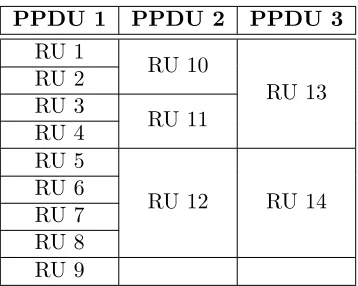
the associated transmission timeτ(µ,ς). . . 45 3.2 Example of RU selection withmk= 14 devices. There are a total ofSk= 3

PPDUs, givenn1 = 9,n2 = 3,n3 = 2 RUs, respectively. . . 54

(14)

List of Figures

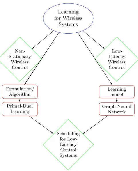
1.1 Design of learning framework for wireless resource allocation problems. Ap-plications are notated with green diamonds, while foundation pillars of the

learning framework are notated with red rectangles. . . 6

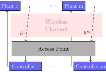
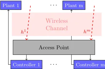
2.1 Wireless control system. Plants communicate state information to access point/controllers over wireless medium. . . 9

2.2 Time axis showing evolution of timetand epochsk. Each channel distribution

Hk is stationary for a set of time instances. . . 9

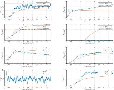
2.3 Convergence paths of optimal values vs. values generated by the Newton

learning method for time-varying H_k for dual variables (left)µ1, (center) ˜µ, and (right) control performance P

Ji₍_yi_{). Newton’s method is able to find}

an approximately optimal value for the dual variables and respective control

performance at each iteration. . . 29 2.4 Comparison of suboptimality (top) and constraint violation (bottom) for the

case of ˆV = 0.01 (left) and ˆV = 0.03 (right). Although the right-hand figures

strive for less accuracy, they perform better because Newton’s method can adapt to the intended accuracy more easily with single iterations. . . 31

2.5 Dynamic evolution of each of the 4 state variables over the time-varying

channel. The blue curve shows the opportunistic power allocation policy found with Newton’s method while the red curve shows the evolution assuming the

loop can always be closed. . . 32

3.1 Wireless control system withmindependent systems. Each system contains a sensor that measure state information, which is transmitted to the controller

over a wireless channel. The state information is used by the controller

(15)

3.2 Multiplexing of frequencies (RU) and time (PPDU) in IEEE 802.11ax

trans-mission window (formally referred as Transtrans-mission Opportunity or TXOP in the standard. The total transmission time is the time of all PPDUs, including

the overhead of trigger frames (TF) and acknowledgments. . . 43

3.3 Inverted pendulum-cart systemi. The statexi,k = [xi,k,x˙i,k, θi,k,θ˙i,k] contains specifies angleθi,k of the pendulum to the vertical, while the inputui,k reflects

a horizontal force on the cart. . . 57

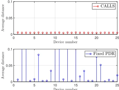
3.4 Average pendulum distance to center vertical for m = 25 devices using (top) CALLS and (bottom) fixed-PDR scheduling with τmax= 1 ms latency

threshold. The proposed control aware scheme keeps all pendulums close to

the vertical, while fixed-PDR scheduling cannot. . . 59 3.5 Total number of inverted pendulum devices that can be controlled using

Fixed-PDR and CALLS scheduling for various latency thresholds. . . 59

3.6 Average ball distance to center for m = 50 devices using (top) CALLS, (middle) event-triggered, and (bottom) fixed-PDR scheduling with τmax= 1

ms latency threshold. The control aware schemes keeps all balancing balls

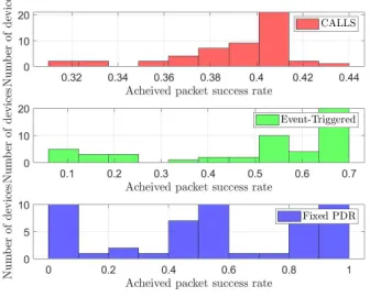
close to center, while fixed-PDR scheduling cannot. . . 61 3.7 Histogram of achieved PDRs inm= 50 balancing board systems (top) CALLS,

(middle) event-triggered, and (bottom) fixed-PDR scheduling with τmax= 1

ms latency threshold. The proposed CALLS method achieves similar PDRs

for all devices, while the fixed-PDR and event-triggered scheduling results in

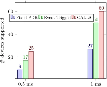
large variation in packet delivery rates. . . 61 3.8 Total number of balancing ball board devices that can be controlled using

Fixed-PDR, Event-Triggered, and CALLS scheduling for various latency

thresholds. . . 62

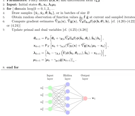
4.1 Typical architecture of fully-connected deep neural network. . . 79

4.2 Neural network architecture used for simple AWGN channel. Each channel

state hi is fed into an independent SISO network with two hidden layers of size 8 and 4, respectively. The DNN outputs a mean µi and standard

deviation σi for a truncated Gaussian distribution. . . 82

4.3 Convergence of (left) objective function value, (center) constraint value, and (right) dual parameter for simple capacity problem in (4.32) using proposed

DNN method with policy gradients, the exact unparameterized solution, and

an equal power allocation amongst users. The DNN parameterization obtains near-optimal performance relative to the exact solution and outperforms the

(16)

4.4 Example of 8 representative resource allocation policy functions found through

DNN parameterization and unparameterized solution. Although the policies differ from the analytic solution, many contain similar shapes. Overall, the

DNN method learns variations on the optimal policies that nonetheless achieve

similar performance. . . 84 4.5 Optimality gap between optimal objective value and learned policy for the

simple capacity problem in (4.32) for different number of usersm and DNN

architectures. The results are obtained across 10 randomly initialized simula-tions. The mean is plotted as the solid lines, while the one standard deviation

above and below the mean is show with error bars. . . 86

4.6 Neural network architecture used for interference channel problem in (4.34). All channel statesh are fed into a MIMO network with two hidden layers of size 32 and 16, respectively (each circle in hidden layers represents 4 neurons).

The DNN outputs means µi and standard deviations σi for i truncated Gaussian distributions. . . 86

4.7 Convergence of (left) objective function value and (right) constraint value

for interference capacity problem in (4.34) using proposed DNN method, WMMSE, and simple model free heuristic power allocation strategies m= 20

users. The DNN-based primal dual method learns a policy that achieves close performance to WMMSE, better performance than the other model free

heuristics, and moreover converges to a feasible solution. . . 87

4.8 Comparison of performance using Gamma and truncated Gaussian distribu-tions in output layer of a DNN. . . 88

4.9 Convergence of (left) objective function value and (right) constraint value for

interference capacity problem in (4.35) using proposed DNN method, heuristic WMMSE method, and the equal power allocation heuristic for m= 5 users.

The DNN-based primal dual method learns a policy that is feasible and almost

matches the WMMSE method in terms of achieved sum-capacity, without having access to capacity model. . . 90

5.1 A wireless network with m transmitters (green) andn receivers (blue). The

transmitters send information over a wireless fading channel, with direct links between transmitter and receiver shown in solid lines and the interference

links shown in dashed lines. . . 99

5.2 An illustration of (a) a graph signal colored onto the nodes of graph with grey-colored edges and (b) a graph convolution operation performed on the

(17)

5.3 Performance comparison during training of REGNN form= 20 pairs. With

only q = 40 parameters, the REGNN strongly outperforms the WMMSE algorithm.The network is plotted in top figure, and the achieved sum-rate

over the learning process is shown in the bottom figure. . . 113

5.4 Performance comparison during training of REGNN form= 50 pairs. With only q = 40 parameters, the REGNN strongly outperforms the WMMSE

algorithm. The network is plotted in top figure, and the achieved sum-rate

over the learning process is shown in the bottom figure. . . 115 5.5 Performance comparison of an REGNN that was trained in Figure 5.4 in

another randomly drawn network of equal size. The top figure plots the

geometric configuration of the new network. The bottom figure shows the empirical distribution of the sum-rate achieved over many random iterations

for all heuristic methods. . . 116

5.6 Empirical histogram of sum rates obtained by (top, blue) REGNN trained on network of size m= 50 and (bottom, red) REGNN trained on network

of size m0 = 75 on 50 randomly drawn networks of size of m0 = 75. The

REGNN trained on the smaller network closely matches the performance of the REGNN trained on the larger network . . . 117

5.7 Empirical histogram of sum rates obtained by (top, blue) REGNN trained on network of size m= 50 and (bottom, red) REGNN trained on network

of size m0 = 100 on 50 randomly drawn networks of size of m0 = 100. The

REGNN trained on the smaller network closely matches the performance of the REGNN trained on the larger network . . . 117

5.8 Performance of REGNN trained in Figure 5.4 in randomly drawn networks of

varying size. From networks of sizem0 = 50 to 500, the REGNN is able to outperform the heuristic methods. . . 118

5.9 Performance of REGNN trained in Figure 5.4 in randomly drawn networks of

varying densities from factors ranging from r= 0.1 to 10. As the density of the network increases, the REGNN is unable to match the performance of

the WMMSE algorithm. . . 119

5.10 Performance comparison during training of REGNN for multi-cell interference network with m= 50 users and n= 5 base stations. With q= 40 parameters,

the REGNN outperforms the model-free heuristics but does not quite meet

the performance of WMMSE, which utilizes model information in its imple-mentation. The top figure plots the geometric configuration of the network,

(18)

5.11 Performance of REGNN trained in Figure 5.10 in randomly drawn multo-cell

networks of varying size. From networks of size 5 to 50 cells, the REGNN matches the performance of the best performing heuristic method. . . 120

5.12 Convergence of training of an REGNN for the wireless sensor network problem

withm= 30 sensors/transmitters. In the top figure, we show the constraint violation for each of the transmitters converges to a feasible solution. In the

bottom figure, we show the objective function converge to a local maximum. 121

6.1 A series of independent wireless control systems send state information over a shared wireless medium to a base station, where control information is

fed back to the systems. The uplink transmissions (red arrow) is subject to

latency constraint tmax. . . 125

6.2 Scheduling architecture of m = 4 users—colored in green, blue, red, and

yellow—acrossn= 3 channels. The total transmission length varies across

channels. The channels need not be located on consecutive frequency bands, and are placed as such here only for the purposes of illustration. . . 125

6.3 Convergence of (left) transmission time for a low-latency, control aware scheduling policy over the learning process. The DNN parameterized

schedul-ing policy obtains feasible latency-contained schedules (tmax= 5×10−4 shown

in dashed red line) on both channels. In the (right) image, we simulate the control system using the learned scheduler and two baseline model-free

heuristic scheduler. The NN policy keeps 8 systems stable, while RR and PR

keep 6 and 0, respectively. . . 134

7.1 Outline of future extensions to learning framework for wireless resource

(19)

Chapter 1

Introduction

The advent of the Internet of Things (IoT) brings way towards the rise of integrating fully autonomous systems into our infrastructure and daily lives. With applications ranging from

industrial robotics to smart grid to autonomous vehicles, the future of these technologies

invariably depend up our ability to increase the capacity of the underlying technology of autonomous IoT systems to support their increasing scale and complexity. One of the most

fundamental of such underlying technologies is our wireless communication systems [7,79,128].

Indeed, a primary feature of future autonomous systems is their ability to communicate sensing and actuation information over the wireless medium—whether it be through 5G,

LTE, Bluetooth, etc.—to make autonomous decisions. It is thus increasingly necessary to

optimally design wireless systems that can support the various demands—e.g. capacity, latency, throughput, etc.—placed by these autonomous systems.

The defining feature of wireless communication is fading, or the various random

disturb-ances experienced by the signal as it propagates through the air. The role of optimal wireless system design is to allocate resources across fading states to optimize long term system

properties. Mathematically, we have a random variableh that represents the instantaneous fading environment, a corresponding instantaneous allocation of resources p(h), and an instantaneous performance outcomef p(h),h

resulting from the allocation of resourcesp(h) when the channel realization is h. The instantaneous system performance tends to vary too rapidly from the perspective of end users for whom the long term averagex=Ef p(h),h

is a more meaningful metric. This interplay between instantaneous allocation of resources

and long term performance results in distinctive formulations where we seek to maximize a

utility of the long term average xsubject to the constraintx=Ef p(h),h. Problems of

this form range from the simple power allocation in wireless fading channels – the solution of

which is given by water filling – to the optimization of frequency division multiplexing [126], beamforming [8, 112], and random access [61, 62].

(20)

is because of the high dimensionality that stems from the variable p(h) being a function over a dense set of fading channel realizations and the lack of convexity of the constraint x = Ef p(h),h. For resource allocation problems, such as interference management,

heuristic methods have been developed [18, 111, 130]. Generic solution methods are often

undertaken in the Lagrangian dual domain. This is motivated by the fact that the dual problem is not functional, as it has as many variables as constraints, and is always convex

whether the original problem is convex or not. A key property that enables this solution is

the lack of duality gap, which allows dual operation without loss of optimality. The duality gap has long being known to be null for convex problems – e.g., the water level in water filling

solutions is a dual variable – and has more recently being shown to be null under mild technical

conditions despite the presence of the nonconvex constraint x= Ef p(h),h [103, 136].

This permits dual domain operation in a wide class of problems and has lead to formulations

that yield problems that are more tractable, although not necessarily tractable without resorting to heuristics [31, 42, 47, 76, 92, 124, 138]. All such approaches invariably require accurate system models and may require prohibitively large computational complexity for

each allocation decision.

In contrast to such model-based heuristics, more recent work has applied machine learning and regression techniques to solve resource allocation problems. Machine learning methods

train a generic learning model, most commonly a deep neural network (DNN), to make resource allocation decisions for a wide variety of problems. One such approach follows the

tenants of supervised learning, or in other words fitting a neural network to a training set of

solutions obtained using an existing algorithm [70, 115, 121, 131]. These techniques are useful in their simplicity and relative effectiveness—neural networks are well suited for finding

good local minima in loss functions typically used in supervised learning, e.g. Euclidean loss.

However, supervised learning techniques are limited by both the availability of solutions needed to build a training set as well as the accuracy of such solutions. The former limitation

implies supervised learning can only be used in resource allocation problems with existing

heuristic solutions, while the latter limitation implies that the learning model will only meet the performance of such heuristics but never exceed them. For many of the open problems

in wireless autonomous system design, a training set required to perform supervised training

methods is unavailable.

A crucial observation in the understanding of wireless resource allocation problems and

their connection to machine learning is the fact that the expectation Ef p(h),h has a

form that is typical of learning problems. Indeed, in the context of learning,h represents a feature vector, p(h) the regression function to be learned, f p(h),h

a loss function to

be minimized, and the expectationEf p(h),hthe statistical loss over the distribution

(21)

the statistical loss with stochastic optimization methods which merely observe the loss

f p(h),h at sampled pairs (h,p(h)). In this way, we follow the interpretation of wireless autonomous system design as aconstrained learning problem, in which we seek a resource allocation function, or policy, that minimizes a statistical loss that represents the physical

performance of the system, subject to the necessary constraints.

In Chapter 2, we present our first method to exploit this interpretation in tackling the

problem of the non-stationarity of wireless channels in practical systems. The optimal resource allocation policy to close a series of wireless control systems is inherently linked to the statistics of the wireless channel. In most practical applications, the statistics will

invariably change over time. To address this problem, we utilize the statistical learning

interpretation of resource allocation to leverage ideas of empirical risk minimization (ERM). ERM substitutes the statistical loss with a deterministic, empirical loss. With the application

of second order convex optimization methods, we demonstrate how we can quickly adapt

the resource allocation policy as the wireless channel distribution changes over time. We proceed in Chapter 3 to apply techniques from machine learning in studying another

wireless resource allocation problem of growing interest in autonomous system design—

namely, the challenge of designing ultra-reliable, low-latency communications (URLLC). As in Chapter 2, we may formulate a constrained resource allocation problem that models

the performance of a resource allocation decision relative to the expected performance of the control system. In such a manner, the resource allocation is a scheduling policy

that minimizes total latency while meeting a control performance constraint. For added

practical value, we look specifically at a formulation employing the IEEE 802.11ax WiFi architecture. The combinatorial size of the scheduling decision space inspires the use of

so-calledassignment methods to find solutions to the resulting optimization problem. While these initial approaches for solving complex wireless resource allocation problems prove effective, they are limited in that they are custom designed to tackle specific problems

in wireless autonomous systems, and moreover utilize a large degree of model information. In

this thesis, we are ultimately interested in developing a comprehensive learning framework for addressing open wireless resource allocation problems. This requires both the generality in

the algorithmic approach, as well as an ability to operate when knowledge of the model—e.g.

system dynamics, capacity model, etc.—-is unavailable, as is most often the case in complex systems of practical interest.

A more promising approach in learning for resource allocation uses the learning model,

e.g. deep neural network, to directly parameterize the resource allocation policy in the optimization problem [25, 38, 69, 73, 83, 132]. This can be considered unsupervised in that

such techniques can train neural networks with respect to an arbitrary system performance

(22)

reinforcement learning. These techniques are further beneficial in that they can be applied

to any arbitrary resource allocation problem and have the potential to exceed performance of existing heuristics. This setting is typical of, e.g., reinforcement learning problems [117],

and is a learning approach that has been taken in severalunconstrainedproblems in wireless optimization [25, 93, 94, 134]. In general, wireless optimization problems dohave constraints as we are invariably trying to balance capacity, power consumption, channel access, and

interference. We develop such a constrained learning framework in Chapters 4 and 5 of this

dissertation.

In Chapter 4, we formally draw an equivalence between resource allocation problems

and constrained statistical learning—or constrained regression—to develop a theoretical and

algorithmic framework for learning resource allocation policies for a generic class of resource allocation problems. In particular, this involves using the universal approximation properties

of fully connected neural network (FCNNs) is to recover the duality results of [103, 136].

From there, we present a so-called primal-dual learning method that can be used to learn the optimal weights of the FCNN for a generic class of resource allocation problems. We

moreover demonstrate how the proposed primal-dual method can be performed model-free,

or agnostic to particular system model knowledge.

The primal-dual framework provides an algorithmic approach for training learning

parameterizations of a resource allocation policy. The next question of interest concerns precisely which learning parameterizations are best suited for representing resource allocation

policies. FCNNs are an immediate candidate due to their general universality property—that

is, they can theoretically approximate any continuous function arbitrarily well. However, just as FCNNs are made a naturally viable choice from their universality property [38, 115],

so too are they limited. The practical challenge of training FCNNs to parameterize strong

performing policies is well documented in empirical study , as their full expressive power inherently requires performing optimization over a very high dimensional space. Moreover,

the completely generic structure of FCNN contains no intrinsic invariance to input scaling or

variation; any change in wireless network size or shuffling of the network labels renders the current FCNN-based policy ineffective. Convolutional neural networks architectures (CNNs),

on the other hand, have proved a solution to this problem for many learning domains such as

image classification and recommender systems by preserving invariances in the architecture itself. While some existing work has used CNNs for wireless resource allocation [69, 121, 131],

they utilize standard temporal or spatial CNNs and thus do not leverage the true invariances

present in wireless networks. In particular, the structure—and subsequent invariances—of wireless networks comes from the links between transmitters and receivers that result from

fading. The work in [23] uses spatial CNNs that utilize the geometric structure of the

(23)

we incorporate a recent development in CNNs that perform convolutions on arbitrarily

structured data—called graph neural networks [45, 55]—to fully utilize the network of fading links in parameterizing a resource allocation policy. When such learning architectures are

used in conjunction with the model-free algorithmic learning approach developed in Chapter

4, we obtain a more complete framework for learning effective resource allocation policies in large wireless systems for application in autonomous system settings.

We conclude in Chapter 6 to apply the developed learning framework in the low-latency

wireless control system problem previously tackled in Chapter 3. In this chapter, we demonstrate how a scheduling problem to address low-latency control systems can be

formulated as the constrained statistical learning problem, and utilize both the primal-dual

learning algorithm and graph neural network parameterization discussed in Chapters 4 and 5, respectively, to solve.

The outline for our developed framework for learning in wireless systems is presented

in Figure 1.1. Chapters 2 and 3 discuss initial applications that utilize machine learning techniques, i.e. empirical risk minimization and assignment methods, to address specific

problems. These applications are shown in green diamonds in the first row of Figure 1.1.

Chapters 4 and 5, shown in the following row in red rectangles, develop the two pillars of a specific framework for addressing generic resource allocations problems. One pillar

involves the formulation of the resource allocation problem and the resulting algorithm—we discuss the primal-dual learning framework in Chapter 4—and the parallel pillar is in specific

learning architectures and parameterization to utilize in the learning process—we discuss

the use of Graph Neural Networks in Chapter 5. Finally, we utilize these two pillars to again address an application of interest, namely the low-latency wireless control system, in

Chapter 6.

The work presented in this thesis develops a learning framework to be applied to a wide variety of complex and large-scale wireless resource allocation problems. Such problems are

becoming increasingly prevalent in the design of the wireless autonomous systems that will

compose the future of IoT technology and infrastructure. As these problems grow in both scale and complexity, machine learning has an enormous potential to become a fundamental

feature of next generation wireless technology, from 6G [19, 46] to Industry 4.0 [79]. The

methodology proposed here is intended to provide a pathway towards successful application of machine learning technology to communication systems. Indeed, there still exist many

important extensions to be made to fully address the challenges posed by wireless IoT

(24)

Learning for Wireless

Systems

Non-Stationary

Wireless Control

Low-Latency Wireless Control

Formulation/ Algorithm

Learning model Primal-Dual

Learning

Graph Neural Network

Scheduling for Low-Latency Control Systems

(25)

Chapter 2

Empirical Risk Minimization for

Non-Stationary Wireless Control

Systems

2.1 Introduction

The recent developments in autonomy in industrial control environments, teams of robotic

vehicles, and the Internet-of-Things have motivated intelligent design of wireless systems.

Even though wireless communication facilitates connectivity, it also introduces uncertainty that may affect stability and performance. To guarantee performance and safety of the

control application it is common to employ model-based approaches. However wireless

communication is naturally uncertain and time-varying due to effects that are not always amenable to modeling, such as mobility in the environment. In this chapter we propose an

alternative learning-based approach, where autonomy relies on collected channel samples to

optimize performance in a non-stationary environment. The connection between the two approaches is based on the observation that a sampled version of the model-based design

approach can be cast as an empirical risk minimization (ERM) problem, a typical machine

learning problem. Even so, standard techniques developed for solving ERM problems in machine learning do not address the additional challenges present in wireless autonomous

systems, namely the non-stationarity of sample distributions.

The traditional model-based approach is motivated by the desire to build wireless control systems with stability and optimal performance. To counteract channel uncertainties it is

natural to include a model of the wireless communication, for example an i.i.d. or Markov

(26)

characterize that it is impossible to estimate and/or stabilize an unstable plant if its growth

rate is larger than the rate at which the link drops packets [51,56,106,113], or below a certain channel capacity [105, 120]. Additionally models facilitate the design of controllers [22, 41, 63],

as well as the allocation of communication resources to optimize control performance,

for example power allocation over fading channels with known distributions [48, 100], or event-triggered control [5, 54, 80, 81, 101].

In practice wireless autonomous systems operate under unpredictable channel conditions

following unknown time-varying distributions. While one approach would be to estimate the distributions using channel samples and then follow the above model-based design approach,

in this chapter we propose an alternative learning-based approach which bypasses the

channel-modeling phase. We exploit channel samples taken from the time-varying channel distributions with the goal to learn directly the solution to communication design problems.

To apply this approach we exploit a connection between the model-based and the

learning-based design problems. Existing works [20, 47, 49] study related problems in multiple-access wireless control systems and resource allocation problems in wireless systems but under a

stationary channel distribution. These works generally employ first-order stochastic methods,

which have slow convergence rates and hence not suitable for the present framework. A significant challenge remains in how to continuously learn optimal policies over a wireless

channel that is time-varying. This shortcoming of existing sample-based approaches used in [20,47,49] and more general machine learning scenarios motivates the higher-order learning

approach proposed in this chapter. Some existing machine learning methods account for

nonstationarity by optimizing an averaged objective over all time [11, 65, 86]. Our approach differs in that we seek and track optimality locally with respect to the current channel

distribution at every time epoch.

In this chapter we consider a wireless autonomous system where the design goal is to maximize a level of control performance for multiple systems while meeting a desired transmit

power budget over the wireless channel (Section 2.2). The wireless channel is modeled as a

fading channel with a time-varying and unknown distribution, and only available through samples taken over time. We derive in Section 2.2.1 a wireless control problem that finds

optimal power allocation policies for an individual time epoch where the wireless channel

distribution does not change, and then proceed to derive the Lagrange dual (Section 2.2.2). We show in Section 2.3 that the dual of the power allocation problem can be rewritten using

channel samples as an empirical risk minimization problem, a common machine learning

problem in which an expected loss function over an unknown distribution is approximated by optimized over a set of samples. Here the risk is loosely related to how far the current

solution is from the desired optimal power allocation.

(27)

Plant 1 · · · Plant m

· · ·

Controller 1 Controller m

Access Point

h1 _hm

Wireless Channel

Figure 2.1: Wireless control system. Plants communicate state information to access point/controllers over wireless medium.

t=0 10 20 30 40 50 60 70 80 90 ...

H1 H2 H3 ...

Figure 2.2: Time axis showing evolution of timet and epochsk. Each channel distributionHk is

stationary for a set of time instances.

a sequence of ERM problems. We collect and store a window of channel samples taken from

consecutive distributions to reduce sampling complexity and employ Newton’s method to learn new policies quickly (Section 2.4). More specifically, the quadratic convergence rate of

Newton’s method is shown to be sufficient to find approximate solutions to slowly varying

objectives with a single update. Using Newton’s method, we propose an algorithm that uses channel samples to approximate the solution of a power allocation wireless control problem

over a non-stationary channel. We prove that, under specific conditions, the algorithm

reaches an approximately optimal point in a single iteration of Newton’s method (Section 2.5). This result establishes both a suboptimality bound with respect to the sampled problem

(Section 2.5.1) as well as with respect to control performance metric in the wireless control

problem (Section 2.5.2). We additionally show a stability result for a particular problem description common in wireless control systems (Section 2.5.3) and provide considerations for

practical implementation of the method (Section 2.6). These results are further demonstrated

in a numerical demonstration of learning power allocation policies across multiple control systems over a time-varying channel (Section 2.7).

2.2 Wireless Control Problem

We consider a wireless control problem (WCP) with m independent control systems labeled

i= 1, . . . , m, as shown in Figure 2.1. Each control system/agent icommunicates at time t

(28)

by transmitting with power levelpi∈[0, p0]. Due to propagation effects the channel fading

conditions that each system iexperiences, denoted byhi ∈R+, change unpredictably over

time [50, Ch. 3]. Together, the channel fading hi _{and transmit power} _pi _{determine the}

signal-to-noise ratio (SNR) at the receiver for system i, which in turn affects the probability

of successful decoding of the transmitted packet at the receiver. We consider a function

q(hi, pi) that, given a current channel state and transmit power, determines the probability

of successful transmission and decoding of the transmitted packet – see, e.g., [48, 100] for

more details on this model. Transmission are assumed on different frequencies/bands and are not subject to contention – see [47, 49] for alternative formulations.

Because these fading conditions vary quickly and unpredictably, they can be modeled

as independent random variables drawn from distributionH that itself is non-stationary, or time-varying. Channel fading is assumed constant during each transmission slot and

it is independently distributed over time slots (block fading). Furthermore, the channel

distributionH may vary acrosstime epochs, but will in general be stationary within a single time epoch. In particular, consider an epoch indexk= 0,1, . . . that specifies a particular

channel distribution H_k with realization hi_k for system i. In Figure 2.2, we display a time

axis rendering of this model. The state variables change at each transmission slott, while the channel changes at scale k, which will in general contain multiple time steps. This is

to say that we assume that the channel distribution H_k changes at a rate slower than the system evolution, and that within a single time epoch the channel is effectively stationary.

We proceed to derive a formal description of the wireless control problem of interest

within a single time epoch, where the channel is assumed stationary. In Section 2.4 we extend this formulation to the non-stationary setting.

2.2.1 WCP in single epoch

Within a particular time epochk with channel distributionH_k, we can derive a formulation

that characterizes the optimal power allocations between the m control systems so as to maximize the aggregate control performance across all systems, wherep0 reflects a maximum

transmission power of the system. Given a random channel state hi_k∈_R+ drawn from the

distributionHk. We wish to determine the amount of transmit powerpi_k(h_ki) :R+→[0, p0]

to be used when attempting to close its loop—see [48] for details. We note that we are

looking for transmit power as a function of current channel conditions, as the power necessary

to close the loop will indeed change with channel conditions. We assume the current channel gainhi_k is available at the transmitter at each slot, as this can generally be obtained via

short pilot signals—see [48]. Then the probability of closing the loop is given by the value

y_ki :=Ehi k

(29)

The variable yi_k ∈ [0,1] is the expectation of successful transmission over the channel

distributionHk.

Using the variableyi

k we use a monotonically increasing concave functionJi: [0,1]→R that returns a measure of control system performance as a function of the probability of

successful transmission. Such a function can take on many forms and, in general, can be derived in relation to the particular control task of interest. In the following example, we

derive such a measure for a typical wireless control problem setting, namely the quadratic

control performance of a switched linear dynamical system – see, e.g., [51, 106].

Example 1. Consider for example that a control system i is a scalar linear dynamical system of the form

xi_t₊₁=Ai_oxi_t+Biui_t+wi_t (2.2)

wherexi

t∈Ris the state of the system at transmission timet,Aio is the open loop (potentially

unstable) dynamics of the system, ui_t∈_Ris the control input applied to the system at time

t, and w_ti is some zero-mean i.i.d. disturbance process with variance Wi. Consider a given linear state feedback is applied to the system as the control input when a transmission is successful, i.e.,

ui_t=

(

Kixi_t if loop closes

0 otherwise (2.3)

As a result, the system switched between an open loop modeAi_o and a closed loop stable mode

Ai_c=Ai_o+BiKi, as in

xi_t₊₁ =

(

Ai_oxi_t+wi_t if loop closes

Ai_oxi_t+wi_t otherwise (2.4)

The goal is to regulate the system state close to zero, i.e., the system attempts to close the loop at a high rate in order to minimize an expected quadratic control cost objective of the form

lim N→∞

1

N

N−1 X

t=0

E(xit)2 (2.5)

Assuming the control loop in (2.4)is closed with the success probability yi_k in (2.1)at all time steps, it is possible to express the above cost explicitly as a function of yi_k. Using the system dynamics (2.4), the variance of the system state satisfies the recursive formula

E(xit+1)2=yki (Aic)2E(xit)2+ (1−yki) (Aio)2E(xit)2+Wi (2.6)

(30)

Operating recursively and using the geometric series sum, we can rewrite the variance at time t as

E(xit)2 = [yki (Aic)2+ (1−yki) (Aio)2]tE(xi0)2 (2.7)

+Wi1−[y

i

k(Aic)2+ (1−yki) (Aio)2]t 1−[y_ki(Ai

c)2+ (1−yki) (Aio)2]

. (2.8)

As follows from the above expression, the system is stable, i.e., the variance is bounded, if the packet success rate satisfies[yi

k(Aic)2+ (1−yki) (Aio)2]<1 so that the sum above is bounded

– see also [51, 106]. In that case, the state variance as well as the average (2.5)converge to the same limit value, which we can define as our control performance function

Ji(y_ki) =− W

i

1−

yi

k(Aic)2+ (1−yki)(Aio)2

(2.9)

This control performance function satisfies the assumption of concavity, and it is also monotonically increasing because we have added the negative sign in front of the expression. It is also possible to extend this analysis to include a cost on the control input, as is common in the Linear Quadratic Control problem, i.e., replace the cost in (2.5)with E(xit)2+ (uit)2.

Remark 1. In Example 1, observe that the control system performance in (2.5) is a long term objective asymptotically for t→ ∞. As the channel fading distributionHk will change unpredictably in the future it is hard to define an accurate value of this control performance.

As a surrogate, in the above example we write a control system performance in (2.9) with

respect to the current channel distributionHk, i.e., as if this channel distribution is stationary and will not change in the future. Later, in Section 2.5.3 we argue that this approximation

and the power allocation algorithm we develop can indeed guarantee system stability.

To derive the full formulation of the wireless control problem for current channel

dis-tribution Hk, we first define using boldface vectors the set of m channel states hk := [h1_k;h2_k;. . .;hm_k]∼ Hm

k observed by the control systems and the set of power allocation policies pk(hk) := [p1k(h1k);p2k(hk2);. . .;pmk(hmk)]∈ P:= [0, p0]m. We further define the vector of trans-mission probabilities at specific channel statesq(hk,pk(hk)) := [q(h1_k, p1_k(h1_k));. . .;q(hm_k, pm_k(hm_k))] and expected transmission probabilities yk := [yk1;yk2;. . .;ymk] from (2.1). The goal is to selectpk(hk) whose expected aggregate value is within a maximum power budgetpmaxwhile

maximizing the total system performance P

Ji _over _m_{agents. Because} _Ji _{is monotonically}

(31)

following optimization problem.

{p∗_k(h),y∗_k}:= argmax pk∈P,yk∈_Rm

J(yk) :=

m

X

i=1

Ji(yi_k) (WCPk)

s.t. yk ≤Ehk{q(hk,pk(hk))}, m

X

i=1

Ehi_k(p i

k(hik))≤pmax

The problem in (WCPk) states the optimal power allocation policyp∗k(hk) is the one that maximizes the expected aggregate control performance over channel states while guaranteeing that the expected total transmitting power is below an available budgetpmax. We stress

that this only provides the optimal policy with respect to a particular channel distribution

Hk. In the non-stationary wireless setting we are interested in solving (WCPk) for allk.

2.2.2 Dual formulation of (WCPk)

Solving this optimization problem directly has a number of significant challenges. The first

is that the problem is non-convex, in particular due to the first constraint in (WCPk). The second challenge is that the problem is optimized over an infinite-dimensional variablepk(hk). It is very difficult to solve such a problem if there is no assumed parameterization ofp∗_k(hk). We can show, however, from a result in [103] that a naturally occurring parameterization of p∗_k(hk) indeed can be derived from Lagrangian duality theory.

We proceed then to derive the dual problem from the constrained problem in (WCPk).

To simplify the presentation, we first introduce a set of augmented variables, denoted with tildes. Define the augmented vectors ˇq(hk,pk(hk))∈Rm+1 and ˇyk∈Rm+1 as

ˇ

q(hk,pk(hk)) :=

     

q(h1_k, p1_k(h1_k)) .. .

q(hm_k, pm_k(hm_k))

−Pm

i=1pik(hik)]

      ˇ yk :=

     

y_k1

.. .

ym_k

−pmax       . (2.10)

The augmented ˇq(hk,pk(hk)) includes transmission probabilities augmented with the total power allocation while ˇyk includes auxiliary variables augmented with total power budget. Using this new notation, the Lagrangian function is formed as

Lk(pk(hk),yk,µk) := m

X

i=1

Ji(y_ki) (2.11)

(32)

where µk:= [µ1k;. . .;µmk; ˜µ]∈R m+1

+ contains the dual variables associated with each of the

m+ 1 constraints in (WCPk). From the Lagrangian function in (2.11), the Lagrangian dual loss function is defined asLk(µk) := maxpk,ykLk(pk(hk),yk,µk)—see, e.g., [14]—and the corresponding dual problem as

˜

µ∗_k:= argmin

µk≥0

Lk(µk) (2.12)

Lk(µk) :=Ehk

(

max pk,yk

m

X

i=1

Ji(y_ki)+µT_k (ˇq(hk,pk(hk))−yˇk)

)

.

Note in (2.12) that the expectation operator and maximization were exchanged without loss

of generality—see, e.g. [47, Proposition 2]. It is important to stress here the connection between the dual problem in (2.12) with the original problem in (WCPk). While (WCPk)

is indeed not convex, problems of this form can be shown to exhibit zero duality gap under

the technical assumption that the primal problem is strictly feasible and that the channel probability distribution is non-atomic [103]. This implies that the optimal primal variable

p∗_k(hk) in (WCPk) can be recovered from the optimal dual variable ˜µ∗k in (2.12). Thus, the power allocation policy for each agent iis found indirectly by solving (2.12) and recovering as

pi_k(hi_k,µk) = argmax pi

k∈[0,p0]

µi_kq(hi_k, pi_k(h_ki))−µp˜ i_k(hi_k), (2.13)

y_ki(µk) = argmax yi

k

Ji(y_ki)−µi_kyi_k. (2.14)

The optimal policy is subsequently recovered using the optimal dual variable as p∗_k(hk) := [p1_k(h1_k,µ˜∗_k);. . .;pm_k(hm_k,µ˜∗_k)]. Observe that the problem in (2.12) is a simply constrained stochastic problem that is known to always be convex from duality theory, and can be solved

efficiently with a variety of projected stochastic descent methods [12, 26, 29, 47, 49]. Thus, the non-convex, infinite-dimensional optimization problem in (WCPk) can be solved indirectly

but exactly with the convex, finite-dimensional problem in (2.12).

Remark 2. The problem formulation given in (WCPk) that we use in this chapter assumes there is a fixed power budget and the metric to be optimized is a measure of control performance. An alternative formulation of resource allocation that may be more relevant

in some settings would instead fix a bound on the required control performance, typically

derived from a stability margin for the control system. Here the objective would instead be to minimize total power usage, subject to the constraint on control performance. Indeed,

these two problems are very similar when reformulated in the dual domain, and can thus be

(33)

chapter but stress that all the results will apply to this alternative problem as well.

2.3 ERM Formulation of

(WCP

k

)

The stochastic program in (2.12) features an objective that is the expectation taken over

a random variable, and can thus be considered as a particular case of the empirical risk

minimization (ERM) problem. Empirical risk minimization is a common problem studied in machine learning due to its ubiquity in training classifiers, and the same structure appears

naturally in the dual formulation of the WCP. A generic ERM problem considers a convex loss function f(µk,hk) of a decision variable µk ∈Rm+1 and random variable hk drawn from distributionH_kand seeks to minimize the expected lossLk(µk) :=Ehk[f(µk,hk)]. For the WCP in (WCPk), we rewrite the loss function Land associated ERM problem in terms of a functionf(µk,hk) using its dual as

˜

µ∗_k:= argmin

µk≥0

Lk(µk) := argmin

µk≥0

Ehkf(µk,hk), (2.15)

f(µk,hk) :=J(yk(µk)) +µTk (ˇq(hk,pk(hk,µk))−yˇk(µk)).

Typically the distribution Hk is not known by the user, so the expected loss cannot be evaluated directly, but is instead replaced by an empirical risk by takingn samples labeled h1_k,h2_k, . . . ,hn_k ∈ Hm

k, (where hlk := [h

1,l k ;. . .;h

m,l

k ]). In practice, such samples can be obtained through the use of short pilot signals sent from the users to measure channel conditions—see [48]. We then consider the empirical average loss function

ˆ

Lk(µk) := 1

n

X

l=1

f(µk,hlk) := 1

n

X

l=1

f_kl(µk). (2.16)

To characterize the closeness of the empirical risk ˆLk(µk) with nsamples with respect to the expected loss Lk(µk), we define a constantVn called thestatistical accuracy of ˆLk. The statistical accuracyVnprovides a bound of the difference in the empirical and expected loss

for all µk with high probability (i.e. at least 1−γ for some smallγ). In other words, we defineVn to be the constant that satisfies

sup

µk

|Lˆk(µk)−Lk(µk)| ≤Vn w.h.p. (2.17)

The upper bounds on Vn are well studied in the learning literature and in general may involve a number of parameters of the loss functionf as well as, perhaps most importantly,

the number of samplesn. For ˆLk(µk) defined in (2.16), a bound for the statistical accuracy

Vncan be obtained in the order ofO(1/

√

(34)

implies a suboptimality of ˆL∗_k := min ˆLk(µk) of the same accuracy, i.e. |L∗k−Lˆ∗k| ≤2Vn [13].

As is often the case in machine learning problems, the statistical accuracy informs the proper use of regularization terms in the empirical loss function. We can add regularizations

to prescribe desirable properties on the empirical risk ˆLk(µk), such as strong convexity,

without adding additional bias beyond that already accrued by the empirical approximation. In other words, as ˆL∗_k will be of orderVn from the optimal expected valueL∗, any additional

bias of orderVn or less is permissible. With that in mind, we add the regularization term

αVn/2kµkk2 whereα >0 to the empirical risk in (2.16) to impose strong convexity. We can further remove the non-negativity constraint on the dual variables in (2.15) through the use

of a logarithmic barrier. To preserve smoothness for smallµk, we use an -thresholded log

function, defined as

log(µk) :=







log(µk) µk ≥

`2,(µk−) µk < ,

(2.18)

where `2,(µk) is a second order Taylor series expansion of log(µk) centered atfor some small 0< <1. We then use −βVn1T logµk where β >0 as a second regularization term, and obtain a regularized empirical risk function

Rk(µk) := 1

n

X

l=1

f_kl(µk) +

αVn

2 kµkk

2₋_βV

n1T logµk. (2.19)

From here, we can seek a minimizer of the strongly convex regularized riskRk(µk) without explicitly enforcing a non-negativity constraint onµk and find a solution with suboptimality

of orderO(Vn) with respect to (2.15). Such a deterministic and strongly convex loss function

as in (2.19) can be minimized using a wide array of optimization methods [26, 34, 64, 85]. However, all such methods only solve the problem for a particular epoch k, or otherwise

assume a stationary channel distribution H_k as is typical in machine learning settings.

2.4 ERM over non-stationary channel

The ERM problem we are interested in solving in wireless autonomous systems is further

complicated by the non-stationarity of H, making existing solution methods insufficient. This is due to the fact that finding the minimizer to Rk(µ) will only provide an optimal

power allocation for the respective channel distributionH_k. In wireless systems, we instead

mustcontinuously learn optimal policies as the channel varies, or in other words, find optimal points forRk(µ) fork= 0,1, . . .. To formulate the non-stationarity, however, we first define

(35)

did in (2.16), we instead define a more general statistical loss function for a non-stationary

channel using samples from the previous M epochs. We define a windowed empirical loss function ˜Lk(µ) at epochk as

˜

Lk(µ) := 1

M

k

X

j=k−M+1

ˆ

Lj(µ) (2.20)

By keeping a window of samples, we may retain N =M n total samples while drawing only

nnew samples at each epoch. If the successive channel distributionsHk−M+1, . . . ,Hk are not very different, we may expect the old channel samples to still be of interest. We define

the associated statistical accuracy ˜VN as the constant that satisfies

sup

µ

|L˜k(µ)−Lk(µ)| ≤V˜N w.h.p. (2.21)

Here we stress that the bounds on this constant ˜VN are not as easily obtainable or

well-studied as in the stationary setting. Such a bound over non-i.i.d. samples may be dependent upon many parameters such as the sample batch size n, window size M, and

correlation between successive distributions H_j andH_j₊₁. Therefore, finding precise bounds on ˜VN would require a sophisticated statistical analysis and is outside the scope of this work. We instead define a user-selected accuracy ˆV that may estimate the statistical accuracy ˜VN.

We assume that ˆV ≥V˜N, with equality holding in cases where ˜VN is known. Using the same

regularizations introduced previously, we obtain the regularized windowed empirical loss function

˜

Rk(µ) := 1

M

k

X

j=k−M+1

ˆ

Lj(µ) +

αVˆ

2 kµk

2₋_β_V_ˆ₁T _log

µ. (2.22)

We subsequently define ˜µ∗_k := argmin_µR˜k(µ). The definition of the loss function in (2.22) includes the batches ofnsamples taken from the previous M channel distributions

H_k−M+1, . . . ,Hk. This definition is, in a sense, a generalization of the simpler empirical

risk Rk(µ) in (2.19). Observe that, by using a window size ofM = 1, we use only samples from the current channel and recoverRk(µ). In the following proposition we establish the

accuracy of an optimal point of our regularized empirical risk function ˜Rk(µ) relative to the

optimal point of the original dual loss functionLk(µ).

Proposition 1. Consider L∗_k = Lk(µ∗_k) and L˜∗_k = minµ≥0L˜k(µ), and define R˜∗_k := minµL˜k(µ) +αV /ˆ 2kµk2 −βVˆ1T logµ as the optimal value of the regularized empirical

risk. Define V˜N by (2.21). Assuming V˜N ≤Vˆ, the difference |L∗k−R˜

∗

(36)

the order of statistical accuracy Vˆ, i.e. for some ρ >0

|L∗_k−R˜∗_k| ≤2 ˜VN +ρVˆ ≤(2 +ρ) ˆV , w.h.p. (2.23)

Proof: To obtain the result in (2.23), consider expanding and upper bounding |L∗_k−R˜∗|=

discussed. The second term, can be decomposed into the bias introduced by the logarithmic barrier−βVˆ1Tlogµand the bias introduced by the quadratic regularizercV /ˆ 2kµk2_{. The}

former of these is known to produce an optimality bias of (m+ 1)βVˆ [14, Section 11.2.2],

while the latter is known to introduce a bias on the order of O( ˆV) [108]. Combining these, we get a total suboptimality between the regularized risk function optimal and the true

optimal of 2 ˜VN+ρVˆ for some constant ρ >0. As we assume that ˜VN ≤Vˆ, the rightmost

bound in (2.23) follows.

A key observation to be made here is that any exact solution to (2.22) only minimizes

the expected loss Lk to within accuracy ˆV (assuming ˆV ≥ V˜N). There is therefore no need to minimize (2.22) exactly but is in fact sufficient to find a ˆV-accurate solution, as

this incurs no additional error relative to the statistical approximation itself. While many

optimization methods can be used to find a minimizer to (2.22), we demonstrate in the next section that fast second order methods can be used to learnapproximate minimizers—and by Proposition 1 approximately solve (2.15)—at each epoch kwith just single updates as

the channel distributionHk changes, thus tracking near-optimal points at every epoch. This is done by exploiting an important property of second order optimization methods, namely

local quadratic convergence.

Remark 3. Observe in the text of Proposition 1 that we define ˜R∗_k to be the optimal point of the loss function ˜Lk(µk) regularized with a standard log barrier−log(µk), rather than the thresholded barrier−log(µk) used in the definition in (2.22). Indeed, using the thresholded

barrier does not explicitly enforce nonnegativity for values smaller than . However, this

thresholding is necessary to preserve smoothness of the barrier, which will be necessary for the proof of Lemma 1 in Section 2.5. The threshold can be made as small as necessary

to enforce nonnegativity, although this comes at the cost of a worse smoothness constant.

In practice, however, we observe this thresholding to not be explicitly needed and is just included here for ease of analysis. We also stress that the smoothness constant itself does

not play a pivotal role in the proceeding analysis.

2.4.1 Learning via Newton’s Method

In this chapter, we use Newton’s method to approximately minimize (2.22) efficiently as