ANALYSIS AND FORECASTING OF CORONAL MASS EJECTION SPACE WEATHER EFFECTS

DEPARTMENT OF PHYSICS

Mateja Dumbović

ANALYSIS AND FORECASTING OF

CORONAL MASS EJECTION SPACE

WEATHER EFFECTS

DOCTORAL DISSERTATION

FIZIČKI ODSJEK

Mateja Dumbović

ANALIZA I PREDVIÐANJE

UTJECAJA KORONINIH IZBAČAJA

NA SVEMIRSKE VREMENSKE

PRILIKE

DOKTORSKI RAD

DEPARTMENT OF PHYSICS

Mateja Dumbović

ANALYSIS AND FORECASTING OF

CORONAL MASS EJECTION SPACE

WEATHER EFFECTS

DOCTORAL DISSERTATION

Supervisor: dr. sc. Bojan Vršnak

Information on the Supervisor

Bojan Vršnak is employed at the Hvar Observatory, Faculty of Geodesy, University of Zagreb since 1981. He graduated theoretical physics in 1980, obtained a Master of Science degree in the field of Atomic and Molecular physics in 1983, and obtained his Ph.D. degree in the field of Astrophysics (Solar Physics) in 1987 at the Faculty of Science in Zagreb. In 2000 he was was elected to the permanent position of scientific adviser.

His main research area is solar activity, namely eruptive processes in the solar atmosp-here and their influence on the heliospatmosp-here and magnetospatmosp-here of the Earth. He published over 300 scientific papers (141 in the peer reviewed journals indexed in "Current Contents", CC) which were cited more than 3700 times. He published a graduate-studies textbook "Temelji fizike plazme" (eng. Introduction to plasma physics), three astronomy textbo-oks for primary and highschool students, written thirteen chapters in various botextbo-oks, and authored and co-authord a number of scientific-popular articles.

He currently gives lectures within a post-graduate studies at the Faculty of Science in Zagreb. His previous educational experience includes lectures within a graduate studies at the Faculty of Science in Zagreb and lectures a s a guest-professor at the Karl-Franzens University in Graz, as well as supervising a number of graduate, master and PhD thesis. He reviewed more than a hundred scientific papers in various international peer-reviewed journals and a number of foreign research project proposals. He is a member of the Editorial board of the scientific journals "Solar Physics" (Kluwer), "The Scientific World Journal" (Hindawi), "Central European Astrophysical Bulletin", and scientific-popular journals "Čovjek i Svemir" and "Bolid". He is a member of International Astronomi-cal Union (IAU), American GeophysiAstronomi-cal Union (AGU), European AstronomiAstronomi-cal Society (EAU), Committee on Space Research (COSPAR), Joint Organization for Solar Obser-vation (JOSO), Community of European Solar Radio Astronomers (CESRA), Croatian Astronomical Society, and Croatian Physical Society.

I would like to express my deepest grattitude to my supervisor, dr.sc. Bojan Vršnak, for giving me the opportunity to start my scientific career and teaching me (almost) everyt-hing I know.

I would also like to thank all of my other colleagues at Hvar Observatory: Roman, Hrvoje, Domagoj, Davor, Jaša, Tomislav, Nikša and Toni for providing the best possible working environment, in both scientific and humanly aspects.

Special thanks to my colleagues and co-authors of my scientific papers from Zagreb Ob-servatory (Dragan, Darije, Damir, Ivan), University of Graz (Astrid and Manuela), Space Research Institute in Graz (Christian and Tanja), University of Kiel (Bernd), Technical University of Denmark (Susanne and Kristoffer), and Royal Observatory of Belgium (La-ure, Luciano and Andy).

I gratefully acknowledge the European Comission FP7 project No. 263252 "COronal Mass Ejections and Solar Energetic Particles" (COMESEP), Croatian Science Founda-tion project No. 6212 "Solar and Stellar Variability" (SOLSTEL) and Croatian Science Foundations’ "Young researchers’ career development project - training of new doctoral students" funding program for financially supporting the making of this thesis.

My special appreciation goes to my family. Without their continuing support and love, none of this would be possible.

Abstract

Coronal mass ejections (CMEs) are most powerful eruptions in the solar system. They are driven by the energy explosively released from the coronal magnetic field and are often associated with solar flares, representing a dissipative energy release that causes a wide range of electromagnetic emission at different wavelengths, from radio waves to gamma rays. CMEs have strong impact on space weather - they can cause severe problems in the modern human technology and represent a significant factor in human space-born missi-ons planning. Therefore, they are an important element of space weather forecast, which is based on a numerous ground-based and space-born observations, as well as a variety of modeling and empirical forecast methods. Namely, CMEs drive the most intense ge-omagnetic storms and largest short-term depressions in galactic cosmic ray flux, so called Forbush decreases. Both of these are direct consequences of the near-Earth interplane-tary conditions due to CME passage over the Earth. Currently, probabilistic forecast methods turned out to be the most efficient procedure for predicting the geomagnetic storm strength and Forbush decrease magnitude based on the remote solar observations. The presented statistical analysis reveales that both geomagnetic storms and Forbush de-creases are stronger for faster and wider CMEs, associated with stronger flares originating closer to the center of the solar disc, especially when they are involved in a CME-CME interaction. Statistical relationships are employed in empirical statistical modeling based on the geometric distribution, which can provide forecast of the CME related geo- and GCR-effectiveness (i.e. geomagnetic storm strength and Forbush decrease magnitude). The evaluation reveales that the forecast is less reliable if it is more specific, and gives a relatively good prediction whether or not strongest storms (Dst >200 nT) and significant Forbush decreases (F D > 3%) will occur. The main advantage is in the early warning, based on the input parameters that are note necessarily satellite-dependent. Based on the presented research, two online forecast tools have been developed, available at Hvar Observatory web page. In addition, geomagnetic forecast model has been implemented in the "COMESEP alert system", which is the first fully automatic system for detection of CMEs and solar flares, forecasting the CME arrival as well as their potentially hazardous impact.

Key words: Sun – Space weather – Coronal mass ejections (CME) – Cosmic rays – For-bush decreases – Geomagnetic storms

1. UVOD

Koronini izbačaji i Sunčevi bljeskovi su najsilovitiji eruptivni procesi na Suncu te se nerijetko smatraju glavnim pokretačima svemirskih vremenskih prilika. Praćenjem i pre-dviđanjem svemirskih vremenskih prilika, odnosno stanja u međuplanetarnom prostoru, bliskoj okolici Zemlje te njenoj magnetosferi, ionosferi i termosferi bavi se svemirska prog-nostika (eng. "space weather"). Iako je to relativno novo područje istraživanja, usko vezano uz razvoj ljudske tehnologije (posebice svemirskih letjelica), može se tvrditi da je njen razvoj započeo davno prije "doba satelita" sa prvim opažanjima Sunčeve aktiv-nosti. Ljudska tehnologija napredovala je značajno u posljednjem stoljeću te je postala i osjetljivija na Sunčevu aktivnost. Živimo u doba satelita, aviona, elektroenergetskih sustava i svemirskih misija, koje izravno mogu biti pod (negativnim) utjecajem Sunčevih eruptivnih procesa. Stoga je shvaćanje i predviđanje takvih događaja te njihovih učinaka neophodno za moderno društvo.

1.1. Koronini izbačaji

Naziv koronini izbačaji dolazi od engleskog naziva "Coronal mass ejection" (u daljnjem tekstu CME), što je povijesni naziv budući su njihova prva opažanja bila koronagrafima u vidljivom dijelu spektra kao velike količine mase koja je izbačena u međuplanetarni prostor. CME-ovima su često pridruženi Sunčevi bljeskovi te eruptivne prominencije. Sunčevi bljeskovi su disipativni procesi u kojima se oslobađa energija u praktički cijelom spektru elektromagnetskog zračenja - od radiovalnih duljina do gama zračenja. Promi-nencije čini hladnija i gušća kromsferska plazma, koju unatoč gravitaciji magnetsko polje zadržava u toplijim i rjeđim višim slojevima Sunčeve atmosfere (koroni). Iako ne postoji jedan-na-jedan povezanost između CME-ova, bljeskova i prominencija, široko je prihva-ćeno stajalište da su to usko povezane manifestacije jedinstvenog fizikalnog procesa, kojeg pokreću nestabilnosti magnetskog polja. Njihov nastanak opisuje se tzv. "standardnim modelom bljeska".

Prema standardnom modelu bljeska, magnetska arkada eruptira uslijed gubitka ravno-teže, te biva izbačena velikom brzinom u međuplanetarni prostor. Pritom, uslijed "razvla-čenja" silnica u okolini arkade, dolazi do njihovog "prespajanja", što u konačnici rezultira preustrojem magnetske strukture. Proces prespajanja silnica uzrokuje impulzivno zagri-javanje plazme te stvaranje čestičnih snopova koji u interakciji s okolinom zrače u gotovo

može ostati "zarobljena" plazma nižih slojeva Sunčeve atmosfere, koja je stoga hladnija i gušća od okoline (eruptivna prominencija). Gibanje magnetske arkade pak gomila plazmu ispred sebe, što u koronagrafu vidimo kao nakupinu mase koja se giba u smjeru suprot-nom od Sunca (CME). Standardni model bljeska je, uz odgovarajuće reference, detaljnije opisan u poglavlju 1.1.2.

Općenito Opažanja podupiru model standardnog bljeska. Iako se opažaju CME-i bez popratnih bljeskova te bljeskovi bez popratnih CME-a, CME-i najveće energije gotovo uvijek su popraćeni snažnim bljeskovima, a vrlo često i eruptivnim prominencijama kao i raznim drugim poremećajima vidljivim u Sunčevoj koroni (detaljnije u poglavlju 1.1.1). Ova opažanja korisna su s aspekta svemirske prognostike, budući da pridruženi Sunčev bljesak može dati dodatne informacije o CME-u koje nisu dostupne iz koronagrafskih opa-žanja. Naime, budući je u koronagrafskim opažanjima Sunčev disk zasjenjen, nemoguće je odrediti područje na Sunčevom disku iz kojeg je erupcija krenula, što u konačnici otežava i određivanje smjera kretanja CME-a.

Međuplanetarni CME-ovi (eng. Interplanetary coronal mass ejection, ICME) uobiča-jeno se opažaju u in situ mjerenjima kao poremećaji niza parametara Sunčevog vjetra i međuplanetarnog magnetskog polja. Povezivanje in situ mjerenja ICME-a s "remote" opažanjima CME-ova na Suncu nije jednostavan zadatak, budući uključuje kompleksnu i nedovoljno razjašnjenu kinematičku evoluciju CME-a. Na većim udaljenostima od Sunca (≈ 20Rsun) propagacija ICME-a pod utjecajem je aerodinamičkog otpora koji

prilago-đava brzinu CME-a Sunčevom vjetru. Aerodinamični otpor kvalitativno vrlo uspješno opisuje propagaciju ICME-a, međutim kvantitativno je ograničen parametrima CME-a i Sunčevog vjetra, čije je određivanje vrlo zahtjevno i nedovoljno precizno. Kinematiku i propagaciju ICME-a dodatno kompliciraju interakcije dva ili više CME-a, određivanje smjera CME-a te odstupanja od originalnog smjera gibanja, što u konačnici može dovesti do pogrešnog određivanja vremena naleta ICME-a. Detaljniji opisin situ i propagacijskih svojstava ICME-a, sa odgovarajućim referencama, dan je u poglavlju 1.1.3.

1.1. Utjecaj koroninih izbačaja na svemirske

vremen-ske prilike

Prilikom heliosferske propagacije ICME-ovi interagiraju s magnetskim poljima i nabi-jenim česticama koje susreću. Međudjelovanje ICME-a sa Zemljinim magnetskim poljem uzrokuje geomagnetske oluje. Ti poremećaji geomagnetskog polja mogu uzrokovati mnoge negativne posljedice na ljudsku tehnologiju. Geomagnetske oluje mogu nastati ukoliko je orijentacija magnetskog polja ICME-a povoljna za magnetsko prespajanje sa geomag-netskim poljem, odnosno ako postoji jaka južna komponenta magnetskog polja. Uslijed magnetskog prespajanja oslobađa se energija te nabijene čestice iz Sunčevog vjetra ulaze duboko u Zemljinu magnetosferu formirajući električne struje u magnetosferi i ionosferi.

index), koji mjeri poremećaje horizontalne komponente na dipolnom ekvatoru. ICME-i mogu uzrokovati jake ili slabe geomagnetske oluje, odnosno biti jako ili slabo geoefektivni, međutim također ne moraju uopće biti geoefektivni. Geoefektivnost ICME-a posljedica je magnetskog prespajanja sa geomagnetskim poljem te stoga ovisi o konvektivnom elek-tričnom polju Ey =v ·Bs, gdje je Bs južna komponenta magnetskog polja ICME-a, a v

brzina Sunčevog vjetra. Svemirske letjelice u L1 lagrangeovoj točki omogućuju direktna mjerenja Bs iv, međutim samo ≈1 sat unaprijed, što uvelike ograničava "vrijeme

reagi-ranja". Budući nas trenutno razumijevanje CME-a i ICME-a ograničava u predviđanju parametara ključnih za određivanje geoefektivnosti ICME-a, nameće se statistički pris-tup - pridruživanje svojstava CME-a opaženih tijekom erupcije na Suncu geomagnetskom odzivu na Zemlji. Detaljniji opis nastanka geomagnetskih oluja, indeksa geomagnetske aktivnosti te geoefektivnosti ICME-ova i CME-ova, uz odgovarajuće reference, nalazi se u poglavlju 1.2.1.

Međudjelovanje ICME-a sa galaktičkim kozmičkim zračenjem uzrokuje kratkotrajna smanjenja toka kozmičkog zračenja koja nazivamo Forbushevim smanjenjima. Forbu-sheva smanjenja mogu biti indikacija prolaska ICME-a kada druga mjerenja nisu dos-tupna (npr. prije doba satelita) te su zanimljiva s aspekta svemirskih putovanja. Nadalje, velike geomagnetske oluje gotovo su uvijek popraćene i intenzivnim smanjenjem kozmič-kog zračenja, stoga predviđanje Forbushevih smanjenja može unaprijediti predviđanje geomagnetskih oluja. Forbusheva smanjenja se mogu mjeriti detektorima na Zemlji (npr. neutron monitorima) i na svemirskim letjelicama u čitavom međuplanetarnom prostoru, kao i na drugim planetima (npr. Marsu). Mjerenja na Zemlji otežana su zbog geomagnet-skog polja i međudjelovanja kozmičkog zračenja s atmosferom, međutim prikladnija su za mjerenja vrlo intenzivnih događaja, za razliku od mjerenja svemirskih letjelica (detaljnije u poglavlju 1.2.2). Modulacija kozmičkog zračenja u heliosferi općenito se može opisati transportnom jednadžbom koja opisuje četiri različita doprinosa: (1) difuziju zbog fluk-tuacija magnetskog polja, (2) drift zbog nehomogenosti magnetskog polja, (3) konvekcija Sunčevim vjetrom te (4) gubitak energije zbog ekspanzije magnetskog polja (odnosno sustava gibanja čestica). Isti fizikalni mehanizmi modulacije primjenjivi su i za opis For-bushevih smanjenja, gdje se u okviru konvektivno-difuzijskog koncepta očekuje ovisnost amplitude smanjenja o magnetskom polju i brzini ICME-a, što je i potvrđeno statističkim studijama. Međutim, slično kao i u slučaju geomagnetskih oluja, predviđanje Forbushevih smanjenja temeljem mjerenja letjelica u L1 lagrangeovoj točki nije dovoljno rano. Nada-lje, zbog sličnih ograničenja i ovdje se nameće statistički pristup, odnosno pridruživanje svojstava CME-a opaženih tijekom erupcije na Suncu odzivu kozmičkog zračenja na Zem-lji. Detaljniji opis modulacije kozmičkog zračenja ICME-ima i CME-ima, uz odgovarajuće reference, dan je u poglavlju 1.2.2.

Za potrebe ovog istraživanja, prikupljen je veliki uzorak događaja. CME-ovima opa-ženima koronagrafima su pridruženi Sunčevi bljeskovi, a potom geomagnetski i odziv kozmičkog zračenja na Zemlji. Parametri CME-a preuzeti su iz SOHO LASCO CME kataloga (opisanog u poglavlju 1.1.1), dok su parametri Sunčevih bljeskova preuzeti iz NOAA kataloga Sunčevih bljeskova detektiranih u X-zračenju (poveznica dana u poglav-lju 2). Promatrani su događaji u vremenskom periodu od 10 siječnja 1996 do 30 lipnja 2011. Sunčevi bljeskovi pridruženi su CME-ima automatskom metodom koristeći vre-menski i prostorni kriterij (detaljnije opisano u poglavlju 2). Potom je izabrano 211 reprezentativnih CME-bljesak parova, gdje su različite brzine CME-a podjednako zastup-ljene u čitavom intervalu 400 km s−1 _{< v <1500 km s}−1 _{i uzeti su svi CME-i sa brzinama} v >1500 km s−1_{. Ovakav reprezentativni uzorak biran je umjesto slučajnog uzorka, jer bi} slučajan uzorak mogao uključivati vrlo mali broj geomagnetskih oluja, koje su vrlo rijetki događaji (u usporedbi s brojem CME-a).

Koristeći dijagrame koji prikazuju mjerenja kinematike CME-a te vremenski niz mjere-nja Dst indeksa, a koji je dostupan u sklopu SOHO LASCO CME kataloga, geomagnetski odziv je pridružen svakom CME-bljesak paru. Pri tom se koristila ekstrapolacija kinema-tičke krivulje do udaljenosti 214 radijusa Sunca, što je srednja udaljenost Zemlje od Sunca. Time je određeno približno vrijeme dolaska ICME-a na Zemlju. Zbog utjecaja aerodina-mičkog otpora i smjera CME-a, geomagnetski odziv je tražen u vremenskom intervalu oko približnog dolaska ICME-a (detalji mjerenja opisani su u poglavlju 2 i prikazani na slici 2.1). Unutar tog vremenskog intervala tražena su smanjenja Dst indeksa, kao pokazatelj geomagnetske oluje te je mjerena amplituda smanjenja Dst indeksa u točki minimuma, gdje je kao referentna točka uzet početak geomagnetske oluje. Amplituda Dst indeksa, Dst, izražena je apsolutnom vrijednošću, dakle poprima pozitivne vrijednosti (iako u vre-menskom nizu Dst indeksa prilikom geomagnetske oluje Dst indeks poprima negativne vrijednosti). Ukoliko unutar vremenskog intervala nije pronađena geomagnetska oluja, mjerena je prva izražena varijacija (Dst > 10 nT) najbliža približnom vremenu dola-ska ICME-a. Za napomenuti je da je kao relevantna geo-efektivnost korištena vrijednost Dst > 100 nT, dakle događaji koji nisu uzrokovali značajnu geomagnetsku oluju ili uopće nisu stigli do Zemlje se ne smatraju geo-efektivnima.

Za svaki CME u uzorku određen je parametar interakcije, koji opisuje mogućnost in-terakcije sa nekim drugim CME-om. U tu svrhu postavljena su tri kriterija CME-CME interakcije: (1) kinematički kriterij prema kojem dva CME-a mogu interagirati ukoliko im se kinematičke krivulje sijeku, (2) vremenski kriterij prema kojemu dva CME-a mogu interagirati ukoliko eruptiraju u "razumnom" vremenskom razmaku te (3) kriterij izvoriš-nog područja i širine prema kojem dva CME-a mogu interagirati ukoliko dolaze iz bliskih područja na vidljivom Sunčevom disku i/ili su relativno široki. Bitno je napomenuti da

interakcije, te da oni nisu usko specificirani, parametar interakcije, i, može poprimiti če-tiri vrijednosti: 1-nema interakcije, 2-interakcija nije izgledna, 3-interakcija je izgledna te 4-interakcija je vrlo izgledna. U slučajevima kada je i= 3,4 u uzorku je zastupljen samo jedan događaj, kojeg karakteriziraju parametri najbržeg interagirajućeg CME-a te mu je pridružena širina najšireg CME-a. Određivanje parametra interakcije detaljno je opisan u poglavlju 2 te slikom 2.2.

Uzorak od 211 CME-bljesak-Dst događaja (u daljnjem tekstu Dst lista) nadopunjen je događajima koji opisuju odziv kozmičkog zračenja na Zemlji. U tu svrhu korištena su mje-renja neutron monitora (NM) na površini Zemlje, korigirana prema utjecaju atmosferskog tlaka i normirana na "mirni" period kada nema velikih promjena u toku kozmičkog zrače-nja. Na taj način amplitudu Forbushevog smanjenja, FD, moguće je mjeriti u postocima. Odziv je tražen u vremenskom periodu 5 dana prije te 15 dana nakon zabilježene Dst anomalije. Kako bi se smanjio utjecaj dnevnih varijacija toka kozmičkog zračenja upro-sječena su mjerenja 3-4 NM stanice (ovisno o dostupnosti podataka) sličnog rigiditeta, ali smještenih na različitim geografskim duljinama (detalji metode nalaze se u poglavlju 1.2.2). Ova metoda ne uklanja dnevne varijacije u potpunosti, stoga je kao relevantni odziv kozmičkog zračenja korištena vrijednost amplitude F D > 1%. Sukladno terminu "geoefektivnost" za geomagnetski odziv, za odziv kozmičkog zračenja koristit će se termin "GCR-efektivnost" (eng. Galactic cosmic rays, GCR). Za napomenuti je da postoje doga-đaji gdje su dvije uzastopne geomagnetske oluje razlučive jedna od druge, međutim opaža se samo jedno Forbushevo smanjenje. U takvim slučajevima dva su događaja spojena u jedan, kojem je pridružen parametar interakcije i = 4 te odgovarajući parametri bržeg, odnosno šireg CME-a (kao što je prethodno opisano). Također, u nekoliko slučajeva nije bilo odgovarajućih podataka za kozmičko zračenje, stoga uzorak CME-bljesak-Dst-FD sadrži 187 događaja (u daljnjem tekstu FD lista, detaljniji opis nalazi se u poglavlju 2).

3. STATISTIČKA ANALIZA

Statistička analiza fokusirana je na specifične CME-bljesak parametre, koji su povezani sa geo- i GCR-efektivnošću u prijašnjim studijama različitih autora (detaljnije opisano u poglavljima 1.2.1 i 1.2.2). To su početna brzina CME-a, v, širina CME-a, w, vršna vrijednost intenziteta X-zračenja pridruženog Sunčevog bljeska, f, položaj pridruženog bljeska na Sunčevom disku (udaljenost od centra diska), r, te parametar interakcije, i. Niti jedan od promatranih CME/bljesak parametara ne pokazuje snažnu korelaciju sa amplitudom Dst indeksa, Dst, niti amplitudom Forbushevog smanjenja, F D. Stoga je upotrijebljen probabilistički pristup. U tu svrhu korištene su Dst iF D raspodijele, gdje su Dst i F D vrijednosti grupirane u četiri odgovarajuća razreda, koja predstavljaju če-tiri različite razine geo- tj. GCR-efektivnosti. Dst razredi su: |Dst| < 100 nT, 100

F D < 1%, 1% < F D < 3%, 3% < F D < 6% te F D > 6%. CME/bljesak parametri su također podijeljeni u razrede. Podjela u razrede za neke je parametre očigledna, budući su diskretni (npr. parametar interakcije). Kontinuirani parametri podijeljeni su u razrede koji otprilike sadrže jednak broj događaja, dakle nisu ekvidistantni. Stoga se podjela CME/bljesak parametara u slučaju analize Dst i F D distribucija donekle razlikuju. Za svaki razred CME/bljesak parametra načinjena je odgovarajuća Dst tj. F D raspodjela te je određena njena srednja vrijednost. Srednjoj vrijednosti svake raspodjele pridružena je (srednja) vrijednost odgovarajuæeg razreda CME/bljesak parametra te je tražena ko-relacija na ovaj način uprosječenih vrijednosti (detaljnije objašnjenje dano je u poglavlju 3 te na slikama 3.1–3.4). Kao mjera raspršenja unutar pojedinog razreda korištene su standardne devijacije. Također je testirana razina statističke signifikantnosti korištenjem t-testa (eng. two-sample t-test, 2stt), gdje je kao razina signifikantnosti korištena vrijed-nost 0.05 (95% signifikantvrijed-nost). Kako bi dodatno potvrdili dobivene rezultate, koristili smo metodu preklapajućih razreda. Naime, koristeći isti uzorak, ustrojena su dva različita skupa razreda (originalni i alterantivni), stoga se pojedini razredi ta dva skupa preklapaju. Kako bi rezultati statističke analize provedene na originalnom skupu bili potkrijepljeni, alternativni skup mora pokazivati iste tj. vrlo slične rezultate. Originalni i alternativni skupovi CME/bljesak razreda dani su u tablicama 3.1 i 3.2 (poglavlje 3).

Statističkom analizom provedenom u poglavljima 3.1 i 3.2 utvrđeno je da postoji odre-đena povezanost promatranih CME/bljesak parametara i Dst, odnosno FD amplitude u skladu sa prijašnjim istraživanjima (opisanima u poglavljima GMS i FD). U oba slu-čaja (Dst i F D) za sve CME/bljesak parametre zamjećuje se određeni trend, koji prate podaci i originalnih i alternativnih razreda. Međutim, standardne devijacije su vrlo ve-like, što ukazuje na veliko raspršenje podataka i kompleksnu ovisnost Dstodnosno F D o CME/bljesak parametrima. To potvrđuju i rezultati 2stt, gdje je vidljivo da su Dst od-nosno F D raspodjele vrijednosno udaljenih razreda signifikantno drukčije, dok za bliske razrede to ne mora biti slučaj. Na temelju provedene analize zaključeno je da su CME-i koji imaju veću početnu brzinu, koji su širi, čiji pridruženi bljeskovi imaju veću vršnu vrijednost intenziteta X-zračenja i bliže su centru vidljivog diska te kod kojih je izglednija CME-CME interakcija jače geo- i GCR-efektivni. Nadalje, u svrhu predviđanja geo- tj. GCR-efektivnosti opaženog CME-a povezanost CME/bljesak parametara sa Dst, odnosno FD amplitudom je kvantificirana krivuljama koje najbolje opisuju trend podataka (slike 3.1–3.4).

4. EMPIRIJSKI STATISTIČKI MODELI

Rezultati statističke analize iskorišteni su za izradu modela raspodjele vjerojatnosti geo-i GCR-efektgeo-ivnostgeo-i CME-a kojemu je prgeo-idružen set CME/bljesak parametara (v, w, r, f, geo-i). Raspodjele Dst i FD amplituda (Dst i F D), prikazane u poglavljima 3.1 i 3.2 vrlo su

F D raspodijele, modeli se donekle razlikuju - za konstrukciju Dst raspodjele korištena je regularna, a za F D raspodjelu pomaknuta geometrijska raspodjela (jednadžbe 4.1 i 4.2). Obje raspodjele jednostavno je konstruirati ukoliko je poznata srednja vrijed-nost raspodjele (jednadžbe 4.3 i 4.4), koju možemo ocijeniti na temelju relacija dobive-nih statističkom analizom (slike 3.1–3.4). Budući je regularna geometrijska raspodjela definirana za razrede k = 1,2,3,4, ... potrebno je pridruživanje razreda k ←→ Dst:

k = 1 ←→ Dst < 100 nT, k = 2 ←→ 100 nT< Dst < 200 nT, k = 3 ←→ 200

nT< Dst < 300 nT, k = 4 ←→ Dst > 300 nT. Slično, razredi F D pridruženi su raz-ličitim vrijednostima k za pomaknutu geometrijsku raspodjelu: k = 0 ←→ F D < 1%, k = 1 ←→ 1% < F D < 3%, k = 2 ←→ 3% < F D < 6%, k = 3 ←→ F D > 6%. Ras-podjele Dst i F D su modelirane i uspoređene sa stvarnim raspodjelama. Uočeno je da pomaknuta geometrijska raspodjela dobro opisuje stvarnu F D raspodjelu. Istovremeno postoje odstupanja regularne geometrijske raspodjele od Dst raspodjele, stoga su zaDst raspodjelu uvedene dodatne korekcije (detaljno opisano u poglavlju 4.1).

Jedinstvena Dst/F D raspodjela konstruirana je pomoću raspodjela vjerojatnosti za pojedini CME/bljesak parametar (jednadžba 4.8), uz pretpostavke da se CME/bljesak parametri međusobno ne isključuju te da su nezavisni jedan od drugog. Iako posljednja pretpostavka nije sasvim točna (opisano u poglavlju 1.1.1), značajno pojednostavljuje pos-tupak. U oba slučaja uočavamo da su raspodjele vrlo asimetrične te da je uvijek najveća vjerojatnost da CME neće biti niti geo- niti GCR-efektivan, što je i očekivano s obzirom na stvarnu raspodjelu geo- i GCR- efektivnosti korištenog uzorka. Stoga, kako bi se ras-podjela vjerojatnosti upotrijebila za predviđanje Dst odnosno FD amplitude, potrebno je naći granične vrijednosti koje mogu definirati određenu geo- tj. GCR-efektivnost. U tu svrhu, za svaki događaj sa Dst odnosno FD liste, prema CME/bljesak parametrima, izračunata je raspodjela vjerojatnosti tj. dobivene su relativne frekvencije Fr(k) koje

od-govaraju četirima različitim vrijednostima k. Svaka relativna frekvencijaFr(k) prikazana

je u dijagramu za odgovarajući opaženi Dst odnosno F D razred (slike 4.3 i 4.6), gdje su Dst i F D razredi iskazani pomoću vrijednosti k (kao što je objašnjeno prethodno). Budući su k razredi diskretni, različite vrijednosti Fr(k) raspršene su duž linija

kons-tantnog k. Gustoća raspršenih Fr(k) prikazana je korištenjem percentila te je korištena

kao smjernica za određivanje graničnih vrijednosti koje odvajaju različite razine geo- te GCR-efektivnosti (detaljno objašnjeno u poglavljima 4.1 i 4.2). Zbog izrazito malog broja najintenzivnijih geomagnetskih oluja u uzorku, pokazalo se nemogućim odvojiti posljednja dva razreda geo-efektivnosti (200 nT< Dst <300 nT od Dst >300 nT), stoga su ta dva razreda spojena u jedan. Primjenom uvjeta graničnih vrijednosti naDstiF D raspodjelu moguće je dobiti procjenu specifičnog razreda geo- tj. GCR-efektivnosti opaženog CME-a s pridruženim bljeskom, kao što je demonstrirano primjerima u poglavljima 4.1 i 4.2.

Modeli su evaluirani korištenjem trening-uzorka, tj. uzorka na kojem je model "treniran" (Dst i FD liste) kako bi se testirala pouzdanost s obzirom na korištene aproksimacije. Potom je evaluacija izvedena na testnom uzorku, tj. novom, neovisnom uzorku dodatno izabranih i izmjerenih događaja. Testni uzorak sadrži CME-bljesak-Dst-FD događaje u vremenskom periodu 1998-2012 koji se ne nalaze u trening-uzorku, a dobiven je istom metodom mjerenja i pridruživanja kao i trening-uzorak (tj. Dst i FD liste). Predviđanje modela evaluirano je usporedbom sa stvarnim rezultatima koristeći verifikacijske mjere za binarne događaje, koje su definirane prema tablici slučajeva sa četiri moguća ishoda: pogodak, lažno upozorenje, promašaj, te točno odbacivanje (detaljnije opisano u poglavlju 5). Pronađeno je da modeli imaju manje-više istovjetnu razinu točnosti predviđanja za trening- i testni uzorak. Dakle, točnost predviđanja neovisna je o korištenom uzorku te je uglavnom pod utjecajem korištenih aproksimacija. Nadalje, za oba modela utvrđeno je da je predviđanje manje pouzdano što je specifičnije. Model za geomagnetske oluje najuspješniji je u predviđanju vrlo intenzivnih geomagnetskih oluja kada je Dst > 200 nT, dok model za Forbusheva smanjenja najuspješnije predviđa da li će biti značajnijeg efekta, odnosno da li se očekuje F D >3 %. Usporedbom sa drugim modelima utvrđeno je da modeli daju dobra predviđanja s obzirom na korištene ulazne parametre i uspješnost predviđanja drugih modela.

6. KRATAK PREGLED I ZAKLJUČAK

Cilj predstavljenog istraživanja je predvidjeti geo- i GCR-efektivnost opaženog CME-a. Statističkom analizom utvrđeno je da su Dst i FD amplitude veće za brže i šire CME-e, kojima su pridruženi snažniji bljeskovi blizu centra Sunčevog diska, te za koje je izglednija CME-CME interakcija. Pronađene statističke veze upotrebljene su za uspostavu empirij-skog modela, koji se bazira na geometrijskoj distribuciji. Evaluacijom modela utvrđeno je da su modeli manje pouzdani kada se koriste za specifičnije predviđanje te im pouzdanost raste kada se rade "grublje" procjene. Glavne prednosti modela su: (1) ulazni parametri bazirani su na "remote" opažanjima CME-a i Sunčevih bljeskova, što omoguæuje rano upozorenje reda veličine ≈1 dan, te (2) opažanja CME-a i bljeskova potrebna za ulazne

parametre ne moraju nužno biti vršena svemirskim letjelicama. Na temelju predstav-ljenog istraživanja izrađene su internet aplikacije za predviđanje svemirskih vremenskih prilika, koje su dostupne na stranicama Opservatorija Hvar. Nadalje, model predviđanja geomagnetskih oluja uključen je u tzv. "COMESEP sustav upozorenja", prvi u potpu-nosti automatizirani sustav detekcije CME-a i bljeskova te predviđanje njihovog vremena dolaska i potencijalno štetnih učinaka.

Ključne riječi: Sunce – Svemirske vremenske prilike – Koronini izbačaji (CME) – Koz-mičko zračenje – Forbusheva smanjenja – Geomagnetske oluje

1. Introduction 1

1.1. Coronal mass ejections (CMEs) . . . 2

1.1.1. Observational characteristics of CMEs and solar flares . . . 3

1.1.2. CME initiation and the standard flare model . . . 6

1.1.3. Interplanetary Coronal Mass Ejections (ICMEs) . . . 7

1.2. CME-related Space weather effects . . . 10

1.2.1. Geomagnetic storms . . . 10

1.2.2. Forbush decreases . . . 14

2. Data selection, measurement method and event list 19 3. Statistical analysis 25 3.1. The relation between CMEs/flares and geomagnetic storms . . . 28

3.2. The relation between CMEs/flares and Forbush decreases . . . 33

4. Empirical statistical models for space weather forecast 39 4.1. Empirical statistical model for geomagnetic storms . . . 42

4.2. Empirical statistical model for Forbush decreases . . . 47

5. Space weather forecast evaluation 55 5.1. Geomagnetic storm forecast evaluation . . . 57

5.2. Forbush decrease forecast evaluation . . . 59

6. Conclusion and summary 63 A. Appendix 67 A.1. Abbreviations and acronyms . . . 67

1. Introduction

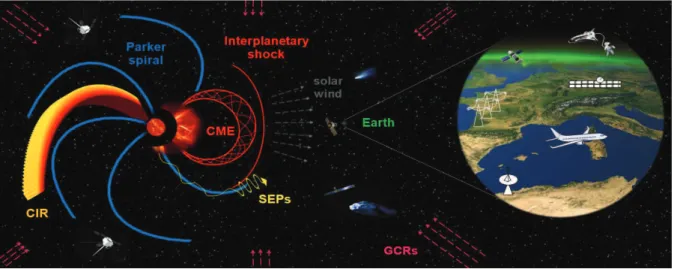
Coronal mass ejections (CMEs) and solar flares are the most violent eruptive processes on the Sun and are often qualified as the main drivers of space weather: "... a field of rese-arch that will provide new insights into the complex influences and effects of the Sun and other cosmic sources on interplanetary space, the Earth’s magnetosphere, ionosphere, and thermosphere, on space- and ground-based technological systems, and beyond that, on their endangering affects to life and health" [Bothmer and Daglis, 2007]. Although space weather is a relatively new research area, tightly connected to the increasing development of the human technology, one may argue that early studies of the solar activity already gave birth to space weather, long before the satellite era. The first recognized space weat-her event was the so-called Carrington event in 1859 when an intensive white-light solar flare was observed for the first time and followed by an intense and broad-range terrestrial responses [Cliver and Svalgaard, 2004]. These terrestrial responses included low-latitude aurorae, as well as the arcing from the induced currents in the telegraph wires in USA and Europe [Tsurutani et al., 2003, and references therein]. The human technology has advanced remarkably in the last century, making us more vulnerable to the solar activity. We live in the era of satellites, airplanes, electrical power grids and space travel, all of which can be affected by solar eruptive phenomena [see e.g.Feynman and Gabriel, 2000]. Therefore, understanding and forecasting of the solar eruptive phenomena and their space weather effects is of great importance for the modern human society.

1.1. Coronal mass ejections (CMEs)

Coronal Mass Ejection (CME) is a historical term for a white-light coronagraphic signa-ture of the mass moving away from the Sun. CMEs were first detected in early 1970-ties by the first space-borne coronagraph that was launched on the satellite Orbiting Solar Observatory, OSO-7. However, their existence was suspected earlier, especially after the discovery of the solar wind (i.e. outflow of mass from the Sun) with in situ measurements of the Mariner 2 probe to Venus in 1962 [see e.g.Howard, 2006, Foukal, 2004].

CMEs are often associated with solar flares and prominence eruptions. Solar flare is a dissipative energy release that causes a wide range of electromagnetic emission at dif-ferent wavelengths, from radio waves to gamma rays. Prominences are cool and dense chromosperic material supported by mgnetic field against the gravity in the hotter and tenuous corona. Although there is no one-to-one relationship between CMEs, flares, and prominences, it is generally accepted that they are closely related and are different manifestations of a single magnetically-driven physical process [Priest and Forbes, 2000]. Therefore, they are described by a unified model called a "standard" flare model, shortly described in Section 1.1.2. There are many observations which support this unified mo-del, as described in Section 1.1.1. In the sense of the space weather forecast, associating CMEs and flares or prominences is a very useful approach, because it provides additi-onal information on CMEs, which cannot be obtained from the white-light coronagraphic observations, as described in Section 1.1.1.

CMEs are observed in the interplanetary space by remote heliospheric imaging met-hods, such asHeliospheric Imager instruments [HI1 and HI2, Eyles et al., 2009] onboard Solar-Terrestrial Relations Observatory spacecraft [STEREO A and B, Kaiser et al., 2008]. Heliospheric imaging of CMEs with STEREO HI instruments theoretically enables tracking the CME from the Sun to Earth, however, this utility is limited by the STEREO’s heliocentric orbit and observational constrains due to projection effects and optically thin medium [see e.g. Vourlidas and Howard, 2006, Rollett et al., 2012, and references the-rein]. Therefore, the best indication of the CME passage at a certain point are stillin situ interplanetary plasma and magnetic field measurements, such as Magnetic Field Instru-ment [MFI, Lepping et al., 1995] ande.g. Solar Wind Experiment [SWE, Ogilvie et al., 1995] instruments onboard Wind spacecraft located at L1 Lagrangian point near Erath. CME in situ properties, as well as their propagation characteristics are shortly described in Section 1.1.3. This internal probing of the interplanetary CME (ICME) provides a unique insight into the CME structure, however, due to the fact that the CME propaga-tion and evolupropaga-tion are still open problems, models and methods are needed to associate remote CME observations at the Sun with the in situ measurements near Earth.

Figure 1.2.: H-alpha (left) and corresponding white-light (right) observation of the ac-tive region AR1271 and a nearby filament with a double solar telescope of Hvar Obser-vatory (22 August 2011).

1.1.1. Observational characteristics of CMEs and solar flares

The eruptive solar phenomena that influence the space weather originate in the solar atmosphere and are driven by the energy stored in the magnetic field. The magnetic structure of the solar atmosphere consists of the "open" and closed magnetic fields and these two types of magnetic structures are associated to different types of phenomena we observe. Coronal holes, i.e. regions of open magnetic field lines are the sources of the high-speed flows in the heliosphere that are of relatively low density [Krieger et al., 1973, Gosling and Pizzo, 1999] and can later form the so-called corotating interaction regions (CIRs, see Section 1.1.3). CMEs originate from the regions of closed magnetic field lines, usually from active regions and quiescent-filament regions. Active regions are structures in the solar atmosphere above sunspots, with enhanced and structured magnetic field, and increased activity compared to the surrounding area. Filaments consist of the colder and denser plasma suspended in the warmer and tenuous solar atmosphere by the magnetic field, appearing darker than the surrounding medium. A filament can be observed in the H-alpha spectral line (Fig 1.2), which forms in the solar chromosphere. When they are observed at the limb, they appear brighter than the dark background and are then referred to as prominences. Quiescent filaments, i.e. prominences can be stable over a time period of months. Eruptive prominences, a special subset of active prominences and often associated with CMEs, can erupt into the high corona in the matter of minutes [Foukal, 2004].

CMEs can be observed directly using white-light coronagraphs, which image the so-lar corona. These are special telescopes where the bright soso-lar photosphere is occulted (imitating a total eclipse) which detect photospheric light scattered by coronal electrons. The observed intensity is therefore determined by the line-of-sight column density so the

Figure 1.3.: White light image of a CME observed by the SOHO LASCO/C2 corona-graph (with a superposed image recorded by EIT/SOHO UV imager in 195 Å) on December 20th 2001 (left) and on February 26th 2000 (right). Both CMEs display a typicall "three-part" structure (Credit: SOHO LASCO CME Catalog).

bright features mowing away from the Sun (CMEs) are interpreted as outward moving density structures [see e.g. Hudson et al., 2006, , and references therein]. Observed CMEs display a variety of morphologies: ranging from narrow jets to wide, seemingly global eruptions [Howard et al., 1985, Webb and Howard, 2012]. It is important to note that CME observations suffer from projection effects, i.e. they are 3D structures pro-jected in two dimensions in an optically thin medium. This introduces distortions in their appearance and complicates the determination of their properties [Burkepile et al., 2004, Hudson et al., 2006]. Therefore, CMEs with large apparent angular width, especi-ally so-called HALO CMEs (with apparent width of 360 degrees), are not actuespeci-ally global eruptions, but are directed close to the Sun-observer line. Around one third of the ob-served CMEs appear as a "three-part" structure (see Fig 1.3), with a bright leading edge, followed by a dark cavity and a bright core [Illing and Hundhausen, 1985]. These observa-tions support the standard CME-flare model (see Section 1.1.2) where the bright leading edge is interpreted as a coronal plasma pileup, the cavity as the magnetic field dominated region and the bright core as the eruptive prominence. This configuration is therefore often viewed as a "standard CME" in both observational and theoretical studies [see e.g. Gopalswamy et al., 2006, , and references therein].

The occurrence of CMEs follows the solar cycle in both phase and amplitude and va-ries by an order of magnitude over the cycle, from ≈ 1 per day in the solar minimum

to ≈ 5 per day in the solar maximum [Webb and Howard, 1994, Schwenn et al., 2006,

Webb and Howard, 2012]. CMEs detected by white-light coronagraphs are characteri-zed by kinematical properties (speed), apparent angular width and a central position angle in the sky plane, measured counter-clockwise from solar north. Measured spe-eds range from a few tens of km/s to nearly 3000 km/s, with an average value which

CME CME

flare

Figure 1.4.: CME detected by the white light coronagraph LASCO/C2 onboard SOHO on August 4th 2011(left), associated solar flare detected in EUV wavelength 193 Åwith AIA instrument onboard SDO (left and middle), and corresponding Soft X-ray flux measured by GOES satellite (right). EUV detection in the middle image is given at the time of the peak in the Soxt X-ray flux seen on the right image. Red line marks the time of the first detection of the CME in C2, as seen in the left image (Credit: SOHO LASCO CME Catalog).

is slightly higher than the ambient slow solar wind speed [≈ 300 and 500 km/s in

the solar minimum and maximum, respectively, see Howard et al., 1985, St. Cyr et al., 2000, Yashiro et al., 2004, Schwenn et al., 2006, Hudson et al., 2006]. The apparent an-gular width of CMEs ranges from a few degrees to more than 120 degrees, with an average value 40-70 degrees [different studies give different values within this range, see Howard et al., 1985, St. Cyr et al., 2000, Yashiro et al., 2004, Schwenn et al., 2006, Webb and Howard, 2012]. CME observations are obtained either by visual inspection of coronagraph images or by automated detection software, resulting in a variety of publi-cally available CME catalogs [listed in Webb and Howard, 2012]. One of the most widely used CME catalogs is SOHO LASCO CME catalog [Yashiro et al., 2004] available at

http://cdaw.gsfc.nasa.gov/CME_list/. The catalog provides CMEs detected in the

field of view of the Large Angle Spectroscopic Coronagraph [LASCO, Brueckner et al., 1995] onboard Solar and Heliospheric Observatory [SOHO, Domingo et al., 1995]. The primary measurements provided by this catalog are performed "manually" on each CME and include the apparent central position angle, the angular width in the sky plane, and the height (heliocentric distance) as a function of time.

Due to the occulting disc, the coronagraph observations of CMEs do not provide infor-mation on the CME source region on the solar disc, which would allow to determine the CME direction. CMEs are often associated with a number of phenomena whose signatu-res can be seen on disc in various parts of the electromagnetic spectrum. These include most notably solar flares, eruptive filaments, waves and dimmings seen in extreme ultra-violet (EUV) imagers and radio bursts [seee.g. Webb and Howard, 2012, and references therein]. One of the most common associations is the one between solar flares and CMEs, relying on the observation that the most energetic CMEs occur in close association with

powerful flares [e.g. Yashiro et al., 2006]. Furthermore, observational and statistical stu-dies have shown that the early kinematical evolution of the CME is related to the energy release in the solar flare [e.g. Kahler et al., 1988, Zhang et al., 2001, Moon et al., 2003, Burkepile et al., 2004, Vršnak et al., 2004a, Maričić et al., 2007]. Therefore, the two can be associated using independent CME and solar flare measurements [e.g. Vršnak et al., 2005], providing the information on the CME source region. An example of the CME and associated solar flare is shown in Figure 1.4.

1.1.2. CME initiation and the standard flare model

In the pre-eruption stage a closed magnetic structure with non-potential magnetic field is generally considered, with stored free energy needed to describe the energy release during the CME/flare event. The most common magnetic structure employed in modeling is a flux rope, a cylindrical plasma structure with magnetic field draped around the central axis [Lepping et al., 1990]. There are observational evidences for flux ropes seen in the early CME initiation phase [Schmieder et al., 2015, and references therein], and their topology is often seen in the interplanetary CME counterparts (see Section 1.1.3. One of the unresolved questions is whether the flux rope is formed below the photosphere and emerges, or is formed above the photosphere by shearing motions or some other physical mechanisms introducing the free energy into the system [e.g. Forbes et al., 2006]. Once emerged or formed, the flux rope either evolves through a series of quasi-equilibrium states or undergoes an abrupt magnetic reconfiguration, both scenarios leading to the loss of equilibrium and the eruption of the coronal magnetic structure, i.e. flux rope [Schmieder et al., 2015, and references therein].

The eruption triggers magnetic reconnection of the overlying coronal magnetic field, a process which can be described as a "...topological restructuring of a magnetic field caused by a change in the connectivity of its field lines." [Priest and Forbes, 2000]. Reconnection can occur above the ejection, or bellow. In both cases the reconnection removes the overlying flux reducing the magnetic tension of the overlying field and enabling a fast outward expansion of the flux rope. When reconnection occurs below the flux rope it feeds it with additional magnetic flux. On the other hand, reconnection releases both thermal and non thermal energy, producing a number of effects, which are all generally described as the solar flare [see e.g. Priest and Forbes, 2002]. The flux rope can support plasma, in which case also an eruptive prominence or filament can be observed. As the erupting flux rope moves away from the Sun, it can produce the disturbances in the local medium, which are observed as coronal waves (extreme ultraviolet, EUV waves) and can form a shock in front of it’s leading edge [see e.g. Warmuth, 2007]. The whole process (also known as the standard flare model) is schematically presented in Figure 1.5. This is a very general view of the CME initiation and many CMEs are not associated with some or even any of the forementioned phenomena (flares, prominences, waves), i.e. low-coronal

prominence shock prominence cavity shock cavity Halpha flare plasma Halpha flare Soft Xray flare plasma pileup/CME Interplanetary shock Coronal shock Coronal wave Eruptive prominence Reconnection region CME wave Halpha flare

Figure 1.5.: A schematic overview of the standard model in 3D view [left, addapted from Forbes, 2000] and side-view [right, addapted from Warmuth, 2007].

signatures. However, even these so-called "stealth" CMEs fit well in the standard model if they are regarded as less-energetic CMEs erupting in the regions of weak overlying field, which then reconfigurates higher up in the corona, where the low density makes the observation of plasma heating challenging [Robbrecht et al., 2009, D’Huys et al., 2014].

1.1.3. Interplanetary Coronal Mass Ejections (ICMEs)

CMEs observed in the interplanetary space using remote heliospheric imaging or in situ measurements are called Interplanetary CMEs (ICMEs). The in situ measurements used for the identification of ICMEs usually include a number of changes in the solar wind and interplanetary magnetic field (IMF) parameters, but highly depend on how the ICME boundaries are defined. A historical approach is very common, where ICME includes the whole disturbance: the shock (if existing), the sheath region, and "driver" or ejecta [see e.g. Rouillard, 2011]. A shock is the discontinuity formed at the leading edge of the CME, when the CME is faster than the surrounding solar wind magnetosonic speed. If present, it is followed by a turbulent and heated sheath region, usually characterized by high plasma density and higher magnetic field strength. Finally, the "driver" or ejecta [which some authors refer to as ICME, e.g. Richardson and Cane, 2010] usually shows some or all of the following signatures: magnetic field enhancement, rotation of the magnetic field, low magnetic field fluctuations, low proton temperature, low proton density, low proton beta parameter (ratio of magnetic and kinetic pressure), monotonic speed decrease, enhanced alpha to proton ratio, elevated oxygen charge states, enhanced Fe charged states, bidirectional electron streaming [see e.g. Zurbuchen and Richardson, 2006, Rouillard, 2011, and references therein]. A schematic of the three-dimensional structure of an ICME relating magnetic field, plasma, and particle signatures is given in Figure 1.6. Magnetic flux ropes are a special subset of ejecta which have magnetic field enhancement and smooth

THE SUN IMF BIDIRECTIONAL ELECTRONS MAGNETIC FLUX ROPE SHOCK EJECTA BIDIRECTIONAL ELECTRONS SHEATH EARTH SHEATH EARTH

Figure 1.6.: A schematic of the three-dimensional structure of an ICME [adapted from Zurbuchen and Richardson, 2006]

rotation of the magnetic field, whereas magnetic flux ropes with low proton temperature and low proton beta parameter are called magnetic clouds [Burlaga et al., 1981].

ICMEs often do not have perfectly clear signatures and thus are often not easily iden-tified in the in situ measurements. Form Figure 1.6 it is quite obvious that depending on the trajectory of the spacecraft through an ICME, different regions will be encountered. If the spacecraft passes through the flank of the ICME, only shock signatures will be observed. On the other hand, if the ICME does not form a shock, only ejecta signatures will be observed. Identification of the ICMEs in the in situ measurements is additionally hampered by CME-CME interaction and stream interaction regions (SIRs). SIRs are regions where a fast solar wind stream interacts with the slow solar wind. Often this region is persistent through couple or even several solar rotations resulting in a so-called corotating interaction region (CIR). A fast solar wind component originates from coronal holes, whereas the slow component originates from regions of closed magnetic field in the solar atmosphere (streamer belts). The spatial variability in the coronal expansion and solar rotation can cause solar wind flows of different speeds to become radially aligned and compressive interaction regions are produced where high-speed wind runs into slower pla-sma ahead [Gosling and Pizzo, 1999]. A defining structure within the CIR is the stream interface, which separates originally kinetically cool, dense, and slow solar wind from what was originally hot, tenuous, and fast solar wind. It is characterized by an abrupt drop in density, a similar increase in temperature, and a small increase in speed [Burlaga, 1974, Crooker et al., 1999]. CIRs can cause similar space weather effects as ICMEs (see Section 1.2), but often to a smaller degree. Therefore, it is important to distinguish between the two using in situ measurements. An example of ICME and CIR identification from the

N p (1 /c m 3 ) N T p (K ) T V p (k m /s ) V p (k B (n T ) B (n T (n T ) DAY d B (n T ) N p (1 /c m 3 ) T p (K ) V p (k m /s ) V p ( B (n T ) B (n B (n T ) d B (n T DAY

Figure 1.7.: In situmeasurements of 24/25 September 1998 ICME (left) and 5 February 2000 CIR [right, both adapted from Dumbović et al., 2012b]. The panels show (top to bottom): solar wind proton density, temperature, and flow speed, magnetic field strength, and magnetic field fluctuations. The red line marks the shock, whereas the gray dotted lines mark the beginning and the end of the ejecta (left). The green line marks the stream interface (right).

in situ measurements is shown in Figure 1.7.

Although ICMEs are undoubtedly related to their solar sources (CMEs), the associ-ation of the two still remains an important scientific issue. Many authors associated CMEs and ICMEs using a variety of different methods, providing CME-ICME lists [e.g. Zhang et al., 2003, Schwenn et al., 2005, Manoharan, 2006, Richardson and Cane, 2010]. However, it should be noted that there are many examples where the associations between different authors disagree. Relating the in situ measurements of ICMEs and their solar sources is not a straightforward task, since it involves a quite complex and not jet fully understood CME kinematical evolution. The CME kinematical evolution is often divided into three phases [Zhang et al., 2001]: the initiation phase, characterized by a slow rise of the magnetic structure; the acceleration phase, characterized by gradual or impulsive acceleration; and propagation phase, showing an almost constant speed in coronagraphic field of view. The forces governing these early kinematic phases are the Lorentz force, gravity and aerodynamic drag, however at larger distances (≈20Rsun) the drag becomes dominant [Cargill, 2004, Vršnak et al., 2004b, 2013]. The drag depends on the CME pro-perties as well as the propro-perties of the ambient solar wind and acts to adjust the CME speed to the speed of the ambient solar wind. Therefore, CMEs faster than the solar wind tend to decelerate, whereas CMEs slower than the solar wind tend to accelerate. A drag based model of the heliospheric propagation of ICMEs has been established [DBM,

Vršnak et al., 2013] which qualitatively describes ICME propagation quite successfully, however, quantitatively it is limited by parameters such as CME speed, width and mass as well as ambient solar wind density and speed, which are not easily derived. ICME pro-pagation is furthermore complicated by the CME–CME interaction [e.g. Temmer et al., 2012], determination of the CME direction and possible deflections of the ICME from the original direction in the corona [e.g. Yashiro et al., 2008, Gui et al., 2011, Möstl et al., 2015] or in the interplanetary space [e.g. Wang et al., 2004, 2006]. The CME direction determines whether or not the ICME will arrive, and whether it will hit with an apex (frontally) or with a flank. The arrival time difference between the ICME apex and flank can be even 2 days [Möstl and Davies, 2013]. Other ICME propagation models are faced with similar challenges and in general the reliability of the propagation models in deriving ICME arrival times is around 10 hours [e.g. Siscoe and Schwenn, 2006, and references therein].

1.2. CME-related Space weather effects

As they propagate through the heliosphere ICMEs can interact with magnetic field struc-tures and charged particles they encounter. The interaction of ICMEs with the geomag-netic field drives geomaggeomag-netic storms, i.e. disturbances of the geomagnetic field. Ge-omagnetic storms are related to many of the previously mentioned harmful effects, and therefore their prediction is an important aspect of the space weather. On the other hand, the interaction of ICMEs with galactic cosmic rays produces short-term depressions in the galactic cosmic ray flux, called Forbush decreases. These depressions can be used as an indication of the ICME passage in the pre-satellite era, when interplanetary measurements were not available. Furthermore, they could be of relevance for the human space missions, where one of the most hazardous factors is a long-term exposure to galactic cosmic rays. Sections 1.2.1 and 1.2.2 shortly describe our current knowledge about geomagnetic storms and Forbush decreases and the physicall processes behind them.

1.2.1. Geomagnetic storms

Geomagnetic storms are recorded by ground-based magnetometers for almost two centu-ries, but the explanation of how and why they occur depended on the discovery of the Earth’s magnetosphere and its interaction with the magnetized solar plasma flow [see e.g. Akasofu, 2007, for historical overview]. Chapman and Ferraro [1931] were the first to introduce the concept of the Earth’s magnetosphere. They suggested that the solar plasma flow forms a comet-like structure around the Earth, extending in the anti-solar direction and confining the Earth and its magnetic field in it. They also predicted the existence of the ring current - a westward flowing current system in the Earth’s mag-netosphere, responsible for the reduction in the horizontal component during the storm. Dungey [1961] was the first to suggest that solar plasma flow is magnetized and that there

MAGNETOPAUSE RECONNECTION MAGNETOTAIL RECONNECTION FLOW IMF FIELDLINES EARTH SOLAR WIND FLOW RECONNECTED FIELDLINES

Figure 1.8.: The concept of the geomagnetic storm based on reconnection between the interplanetary magnetic field lines and geomagnetic field lines at the magnetopause, fol-lowed by a subsequent reconnection in the magnetotail. For a more detailed explanaiton see main text [adapted from Dungey, 1961].

is connectivity between the geomagnetic and interplanetary magnetic field. He proposed that reconnection takes place on the dayside magnetosphere boundary (magnetopause) and that the newly connected field lines are then transported by the solar wind to the magnetotail (magnetosphere extended in the anti-solar direction). Subsequently, the field lines are reconnected there and then transported back to the dayside magnetosphere. This concept is shown in Figure 1.8.

The modern concept of the geomagnetic storm relies on the scheme presented in Figure 1.8. A geomagnetic storm occurs if the topology of the magnetic field in the ICME is favorable for reconnection,i.e., if there is a strong southward component of the magnetic field. As reconnection takes place and energy is released, charged particles originating from the solar wind enter deep into the magnetosphere. As a consequence currents are formed in the magnetosphere and ionosphere - ring current particle fluxes are increased introducing (westward flowing) partial ring currents, and particles are dumped into the high latitude (polar) regions of the Earth as field-aligned currents and (westward flowing) auroral electrojet currents [e.g. Campbell, 2001]. When reconnection stops so does the energy/particle feed as well, and charged particles gradually accumulate in the Earths radiation (Van Allen) belts. The contributions of these currents to ground-based mag-netic recordings are seen as disturbances and are not the same throughout the entire Earth. At high latitudes the field aligned currents and auroral electroject currents do-minate, whereas at low and equatorial latitudes the dominant contribution is from the ring current. At mid-latitudes both ionospheric and magnetospheric currents contribute to the magnetic recordings [Campbell, 2001]. Various measures of the magnetic activity, called geomagnetic indices, are used to describe these geomagnetic field variations and are

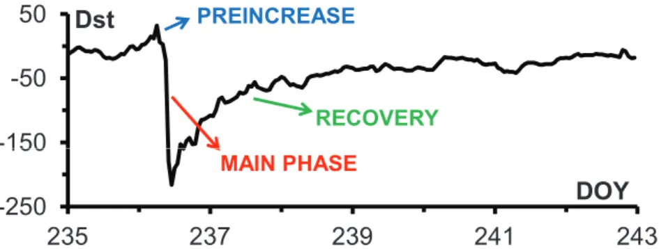
-150 -50 50 _{Dst PREINCREASE} RECOVERY -250 150 235 237 239 241 243 DOY MAIN PHASE

Figure 1.9.: Geomagnetic storm seen in the Dst index on August 24 2005 (data taken from Space Physics Interactive Data Resource, SPIDR).

correspondingly latitude dependent. Auroral electrojet index (AE) is used for the high latitudes, Planetary geomagnetic activity index (Ap) and its discrete equivalentKpindex are used for the mid-latitudes, whereas for low-latitudes Disturbance storm time index (Dst) is used [Campbell, 2001]. The Dst index is derived from the horizontal component recorded by four observatories located between −33 and +30 degree latitude and

repre-sents the axially averaged disturbance of the surface magnetic field at the dipole equator [e.g. Rostoker, 1972, Verbanac et al., 2011a]. The present day concept of geomagnetic storms, as measured by the Dst index, was first established by [Cahampan and Bartels, 1940]. The storm starts with a storm sudden commencement (SSC): a step-function-like increase in the horizontal component (i.e. Dst), and is followed by a main phase: a large and rapid decrease that follows the SSC. After reaching the maximum decrease during the main phase, the storm recovers slowly during the recovery phase. The SSC is caused by the impact of the ICME shock on the magnetosphere, whereas the main phase is caused by the formation of partial ring current. As the partial ring current slowly decays, the Dstindex slowly recovers. An example of the geomagnetic storm as seen in theDstindex is presented in Figure 1.9.

ICMEs display a wide range of geo-effectiveness, i.e. may produce large or small ge-omagnetic storms or none at all. The enhanced geo-effectiveness is related to effective reconnection with the geomagnetic field and therefore with the south component of the ICME magnetic field, Bs and the corresponding y component of the convective electric

field, Ey =vB˙s (wherev is the solar wind speed). The relation betweenin situ properties

of ICMEs and geomagnetic storms has been investigated in statistical studies considering different geomagnetic indices. Dst index was found to correlate with the Bs, a weaker

correlation was found betweenv andDst, and a strong correlation was found betweenDst and Ey [e.g. Kane, 2005, Richardson and Cane, 2011b, Verbanac et al., 2013, and

refe-rences therein]. Most of the intense storms were found to be caused by magnetic clouds with shocks [e.g. Echer et al., 2008, Yermolaev et al., 2012]. In addition, it was found that faster ICMEs have stronger fields, therefore faster ICMEs can enhance both cru-cial geoeffective factors, Bs and Ey [e.g. Gonzalez et al., 1998, Koskinen and Huttunen,

2006, Verbanac et al., 2013]. The approximate threshold value for Ey needed to

pro-duce an intense storm with Dst < −100 nT was obtained empirically [≈ Ey > 5 mV/m

for a duration of 2-3 hours, see e.g. Gonzalez and Tsurutani, 1987, Echer et al., 2008, Richardson and Cane, 2011b]. It should be noted that CIRs can also be geoeffective, howe-ver, they rarely cause intense geomagnetic storms [Dst <−100nT,e.g. Richardson et al., 1996, Verbanac et al., 2011b].

Measurements of Bs needed to estimate Ey are provided at L1 lagrangian point, i.e.

≈1 hour before the start of the disturbance, providing very limited "response time" [e.g.

Koskinen and Huttunen, 2006, Richardson and Cane, 2011b]. Our current knowledge res-tricts us from predicting the crucial Bs component of the ICME magnetic field at earlier

times, e.g. from remote solar observations. There are studies trying to compare the magnetic field of the ICME to its solar source region magnetic fields in the initiation phase [e.g. Bothmer and Schwenn, 1994, Möstl et al., 2008]. However even if the ori-ginal orientation of the magnetic field inside the CME would be known in the initiation phase, the prediction of Bs component at the Earth would be severely hampered by

the fact that CMEs rotate while propagating [e.g. Vourlidas et al., 2011, Isavnin et al., 2013]. Nevertheless, several authors tried to relate remote solar observations of CMEs with geomagnetic storms, assuming that the solar sources of ICMEs (CMEs) must show some properties which can indicate a possible level of the associated geomagnetic activity. These studies led to the conclusion that the geo-effectiveness of CMEs is related to the following solar properties of CMEs and the associated solar flares: CME initial speed [e.g. Srivastava and Venkatakrishnan, 2004, Gopalswamy et al., 2007], apparent angu-lar width [e.g. Zhang et al., 2003, Srivastava and Venkatakrishnan, 2004, Zhang et al., 2007], source region location [e.g. Zhang et al., 2003, Srivastava and Venkatakrishnan, 2004, Gopalswamy et al., 2007, Zhang et al., 2007, Richardson and Cane, 2010], the in-tensity of the CME-related flare [e.g. Srivastava and Venkatakrishnan, 2004], and occur-rence of successive CMEs [e.g. Gopalswamy et al., 2007, Zhang et al., 2007]. However, most of the above studies have samples based on geomagnetic storms observed at Earth, which are then associated to CMEs at the Sun. They do not consider a sample of CMEs at the Sun and then relate them to geomagnetic activity observed at Earth (if there is any). Therefore, they do not take into account so called false and missing alarms. False alarms are CMEs apparently having favorable solar properties, which do not produce geomagne-tic storms, whereas missing alarms are the geomagnegeomagne-tic storms produced by CMEs with apparently non-favorable solar properties [seee.g. Schwenn et al., 2005, Rodriguez et al., 2009]. There were several attempts to construct geomagnetic storm prediction-models ba-sed on the remotely-measured properties of CMEs [e.g. Srivastava, 2005, Valach et al., 2009, Kim et al., 2010, Uwamahoro et al., 2012]. The authors however point out a qu-ite low success rate of the models, unless interplanetary conditions are also taken into account.

-10

0

c

o

u

n

t(

%

)

FIRST STEP (SHOCK) SECOND STEP (EJECTA)

-20

193

196

199

202

205

C

R

DOY

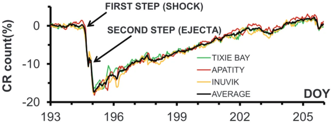
Figure 1.10.: Two-step Forbush decrease detected by ground-based neutron monitors at Earth on July 13 1982. Three high-latitude stations of the similar cutoff rigidity and spaced about equally in longitude are used to minimize daily variations (colored curves). The average of the stations is given by a black curve. Hourly averages of the relative particle counts are presented, normalized to the quiet 1 day period prior to the depression (data taken from Space Physics Interactive Data Resource, SPIDR).

1.2.2. Forbush decreases

Forbush decreases are short term depressions in the galactic cosmic ray (GCR) flux, first observed by Forbush [1937] and Hess and Demmelmair [1937]. There are two types, one caused by CIRs and the other caused by ICMEs. CIRs usually produce shallower and more symmetric depressions [e.g. Iucci et al., 1979, Richardson, 2004] and are often recurrent (due to corotating nature of their interplanetary sources). ICME-related depressions show a variety of shapes and magnitudes, which is generally thought to be related to the characteristics of the ICME part where the detector passes. Depending on the trajectory of the spacecraft through an ICME we expect to see different depressions, similarly as we would expect to see different ICME in situ measurements corresponding to different ICME regions [e.g. Cane et al., 1994, Cane, 2000, Blanco et al., 2013a]. If only ICME ejecta is intercepted the decrease is confined within the duration of the ejecta, whereas the effect of the shock persists many days after the passage of the shock and causes a slow recovery [Cane et al., 1994]. If both the shock and ejecta are intercepted, a two-step decrease is expected, first step coming from the sheath, whereas the second depression is associated with the ejecta [e.g. Barnden, 1973, Cane, 2000, Richardson and Cane, 2011a]. Largest observed Forbush decreases show a two-step structure and the two regions are in average found to be roughly equal in magnitude [Richardson and Cane, 2011a]. However, two-step decreases are not very common and Forbush decreases generally show a diverse and complex structure, even in case when shock/sheath is followed by a single magnetic ejecta [Jordan et al., 2011]. An example of a two-step Forbush decrease is shown in Figure 1.10.

Forbush decreases can be measured in the interplanetary space and by ground based detectors at Earth. Due to the relatively small effect (several percent) a large statistics is

needed,i.e. large particle counts. These are easily provided by large ground based neutron monitors with≈104 _{counts per hour. However, ground based observations are influenced} by several factors: (1) they do not detect primary GCRs, but secondary particles which are the product of GCR interacting with the atmosphere, (2) primary GCRs interact with the geomagnetic field before they enter the atmosphere and the point of their entrance is highly dependent on this interaction, and (3) the GCR flux exhibits daily variations which may represent noise in Forbush decrease measurements. Due to the geomagnetic effect there is a difference in the particle energies of primary GCRs which contribute to different neutron monitor measurements. Particles can enter the atmosphere more easily at poles and high latitudes (where the geomagnetic field is directed toward the atmosphere) than at the equator and low latitudes. Whether or not a particle can enter the atmosphere at a certain point depends on the rigidity, a quantity which depends on the magnetic field strength and particle energy. Depending on the latitude, different neutron monitors have different cutoff rigidities and even the stations close to the pole have cutoff rigidity > 0. Since Forbush decrease is rigidity dependant, i.e. it is more pronounced for low-energy particles [Lockwood, 1971, Cane, 2000] smaller depressions are observed at Earth than in the interplanetary space. Another drawback of using ground based neutron monitor measurements are the daily variations of the detected particle counts. The daily variations are caused by the outward radial convection due to solar wind and an inward diffusion along the direction of the interplanetary magnetic field (see the transport theory description in the next paragraph). The balance between the two generates a small, but significant GCR spatial anisotropy which is observed as the daily variation in the ground-based measurements [≈ 1%, Parker, 1964, Tiwari et al., 2012]. The daily

variations can be reduced by averaging several stations located at approximately same latitude (which roughly have the same cutoff rigidity) and having different asymptotic viewing directions [which roughly correspond to different longitudes, see Dumbović et al., 2011, and Figure 1.10]. Spacecraft observations are not hampered by these effects, but most of them offer much less statistics due to their size and geometric factor. Single counters, which count all particles that enter from all directions, regardless of their energy, provide good statistics [e.g. Cane, 1993, Kühl et al., 2015]. However, these measurements are often contaminated by increased solar energetic particle flux from the ICME shock. Spacecraft measurements are therefore suitable for small Forbush decreases caused by ICMEs without shocks, whereas ground based measurements are more suited for large shock-associated effects.

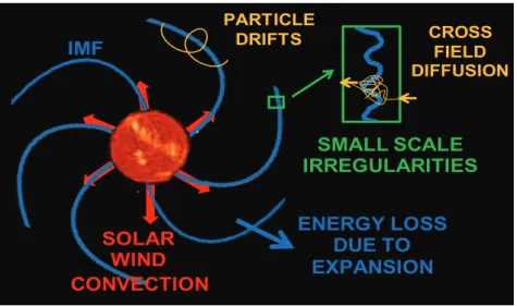
The physical mechanism behind the modulation of cosmic rays can be described in general by a transport equation [Parker, 1965] which combines four different contributions: (1) diffusion across field lines due to magnetic field irregularities, (2) particle drifts, (3) convection by the solar wind, and (4) energy loss due to the expansion of the magnetic field. Parker [1965] proposed that the modulation of GCRs can be explained by their