by Siegfried Heiler 4 Problems of simple kernel estimation and restricted approaches

1

A Survey on Nonparametric Time Series Analysis

by Siegfried Heiler

1 Introduction

2 Nonparametric regression

3 Kernel estimation in time series

4 Problems of simple kernel estimation and restricted approaches

5 Locally weighted regression

6 Application of locally weighted regression to time series

7 Parameter selection

8 Time series decomposition with locally weighted regression

References

1 INTRODUCTION 2

1 Introduction

In this survey we discuss the application of some nonparametric techniques to time series. There is indeed a long tradition in applying nonparametric methods in time series analysis, and this holds not only true for certain test situations, as, e.g. runs tests for randomness of a stochastic sequence, permutation tests or certain rank tests.

An old and established technique in time series analysis is periodogramme analysis. Alt-hough the periodogramme is an asymptotically unbiased estimate of the spectral density of an underlying stationary process, it is well known that it is not consistent. Therefore already in the early fties smoothing the periodogramme directly with a so-called spectral window or using a system of weights, according to a lag window with which the empirical autocovariances are multiplied in the calculation of the Fourier transform, was introdu-ced. Quite a number of dierent windows were proposed and with respect to the window width similar rules hold for achieving consistent estimates as the ones we will shortly dis-cuss in the context of nonparametric regression later in this text. Nonparametric spectral estimation is extensively treated in many textbooks on time series analysis to which the interested reader is refered. Hence it will not be treated further in this survey.

Another area, where nonparametric ideas are being applied since a long time is smoothing and decomposing seasonal time series. Local polynomial regression can be traced back to 1931 (R.R. Macaulay). A. Fisher (1937) and H.L. Jones (1943) discussed a local least squares t under the side condition that a locally constant periodic function (for model-ling seasonal uctuations) be annihilated and already in 1960 J. Bongard developped a unied principle for treating the interior and the boundary part (with and without sea-sonal variations) of a time series derived from a local regression approach. These ideas will be taken up later again in section 8, since they represent an attractive alternative to smoothing and seasonal decomposition procedures based on linear time series models. The aim of this survey is to present some basic concepts of nonparametric regression in-cluding locally weighted regression with the special emphasis on their application to time series. Nonparametric regression has become an area with an abundance in new metho-dological proposals and developments in recent years. It is not the intention of this paper to give a comprehensive overview on the subject. We rather want to concentrate on the basic ideas only. The reader interested in some dierent aspects may be refered to a survey paper by Hardle, Lutkepohl and Chen (1997), where more specic areas, proposals and further references can be found.

The ARMA model is a typical linear time series model. Threshold autoregression (TAR) models and its variates are specic types of nonlinear models. ARCH and GARCH type models are also of a very specic nonlinear type to capture volatility phenomena. In con-trast to that in nonparametric regression no assumption is made about the form of the regression function. Only some smoothness conditions are required. The complexity of the model will be determined completely by the data. One lets the data speak for themselves.

2 NONPARAMETRIC REGRESSION 3

Thereby one avoids subjectivity in selecting a specic parametric model. But the gain in exibility has a price. One has to choose bandwidths. We come back to this later. Besides this, a higher complexity in the mathematical argumentation is involved. However, asym-ptotic considerations will not be discussed in detail in this survey.

Because of their exibility nonparametric regression techniques may serve as a rst step in the process of nding an adequate parametric model. If no such one can be found which describes the underlying structure adequately, then the results of nonparametric estima-tion may be used directly for forecasting or for describing the characteristics of the time series.

2 Nonparametric regression

Since forecasting is an important objective of many time series analyses, estimating the conditional distribution, or some of its characteristics play a considerable role. For point prediction the conditional mean or median is of particular interest. In order to obtain condence or prediction intervals also estimates of conditional variances or conditional quantiles are needed. The latter ones are also of interest in studying volatility in nancial time series.

The rst step to go is therefore to look at nonparametric estimation of densities and condi-tional densities. Let x2IRbe a random variable whose distribution has a density f and

let x1;:::;xn be a random sample from x . Then a kernel density estimator for f is

given by fn(x) = 1_nhn n X i=1 K xi;x hn : (2.1)

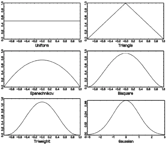
Here K is a so-called kernel function, i.e. a symmetric density assigning weights to the observations xi which decrease with the distance between x and xi. Some

popu-lar kernel functions are listed in Table 2.1 and exhibited in Figure 2.1. The rst 5 have the interval [;1;1] as support, whereas the Gaussian kernel has innite support. hn is

the bandwidth which drives the size of the local neighbourhood being included in the estimation of f at x . The bandwidth depends on the sample size n and has to full hn !0 and nhn!1 for n! 1 as necessary condition for consistency. But for

prac-tical applications this asymptotic condition is not very helpful. A very small bandwidth will lead to a wiggly course of the estimated density, whereas a large bandwidth yields a smooth course but will possibly atten out interesting details. Bandwidth selection will

2 NONPARAMETRIC REGRESSION 4

be dealt with in section 7.

A kn;nearest neighbour (kn;NN) estimator of f is obtained by substituting the

Table 2.1: Selected kernel functions

Name Kernel Uniform 1 2 1I [;1;1](u) Triangle (1;juj)1I [;1;1](u) Epanechnikov 3 4 (1 ;u 2)1I [;1;1](u) Bisquare 15 16 (1 ;2u 2+u4)1I [;1;1](u) Triweight 35 32 (1 ;3u 2+ 3u4 ;u 6)1I [;1;1](u) Gaussian 1 p 2 exp( ; 1 2u 2)

xed bandwidth hn in (2.1) by the random variable Hn;kn(x) measuring the distance

between x and the kn-nearest observation among the xi;i = 1;:::;n:

Nearest neighbour estimators have the property that the number of observations used for the local approach is xed. This is an advantage if the x-space shows a greatly unbalanced design. On the other hand the bias varies from point to point due to the variable local bandwidth.

For x2IR

p _{a kernel K :}

IR

p

!IR is needed in (2.1). In this case either product kernels

K(u) = Yd

j=1

Kj(uj)

with kernels Kj and Kj :IR!IR, bandwidth hj in coordinate j, and hn=h 1

:::hp or

norm kernels

K(u) = K (jjujj)

with a suitable norm on IR

p _{are used. In connection with time series applications}

fre-quently product kernels are applied, fn(x) = 1nXn i=1 p Y j=1 1 hjKj x ij ;xj hj ! (2.2) and hj = ^jh with an estimated standard deviation in the j-th coordinate is a popular

choice for the bandwidths.

Let now (y;x) with y 2IR;x2 IR

p _{be a random vector with joint density f(y;x) and}

let fX(x) be the marginal density of x. Then the conditional density g(yjx) =

2 NONPARAMETRIC REGRESSION 5

Figure 2.1.

nearest neighbourhood estimator in the nominator and denominator of g(yjx). With the

choice of a kernel function K =IR

p+1

!IR; K(y;x) = K

1(y)K(x)

and bandwidths h1 resp. h we obtain the kernel estimator for the conditional density

gn(yjx) = h;1 1 n P i=1 K1 yi;y h1 K xi;x h n P i=1 K xi;x h : (2.3)

An estimator for the conditional mean m(x) = 1 R

2 NONPARAMETRIC REGRESSION 6

g in the integral by its estmator gn. For K1 being a symmetric density this immediately

yields mn(x) = n P i=1 yiK x;xi h n P i=1 K x;xi h : (2.4)

This is the well-knownNadaraya-Watson nonparametric regression estimator(NW-estimator, Nadaraya, 1964; Watson, 1964). We see that it can be written as a weighted mean

mn(x) = n

X

i=1

yiwn;i(x;x1;:::;xn); (2.5)

where the random weights depend on the point x and the random variables x1;:::;xn.

Apart from conditional means also conditional quantiles are of interest in various time series applications. Let

F(yjx) =

y

Z

;1

g(yjx)dy (2.6)

denote the conditional distribution function of y given x. Then the conditional -quantile at x; q(x) is dened as

q(x) = inffy2IR jF(yjx)g; 0 < < 1: (2.7)

If g(jx) is strictly positive, then of course q(x) is the unique solution of F(yjx) = ,

i.e. q(x) = F;1(

jx). One possible procedure for estimating q is to take the empirical

-quantile of an estimator Fn= (jx) according to (2.7).

Let F1(z) =

z

R ;1

K1(u)du be the distribution function pertaining to the kernel K1. Then

the estimated conditional distribution, obtained by integrating gn(jx) from ;1 to y,

is given by Fn(yjx) = n P i=1 K xi;x h F1 y;yi h1 n P i=1 K xi;x h : (2.8)

2 NONPARAMETRIC REGRESSION 7

Let us assume that K1 has support [

;1;1]. Then we have F1 y;yi h1 = ( 1 ; for yi y;h 1 0 ; for yi y + h 1 ; so that in this case

Fn(yjx) = 1 n P i=1 K xi;x h ( n X i=1

1

1

One can see that the estimation contains only observations in the regressor space laying in a band around x. The rst sum on the right hand side includes observations, whose y-values are less than or equal to y ;h

1. The second sum contains observations with

yi-values in a neighbourhood of y. In contrast to a usual empirical distribution function

here also observations greater than y obtain a positive weight.

Of particular interest may be the median regression function q1=2 for asymmetric

distri-butions as an alternative to ordinary regression based on the mean. Another interesting application may be the estimation of q=2 and q1;=2 in order to get predictive intervals.

These can be compared with intervals obtained from parametric models, which lack the possibility to evaluate the bias due to mis-specication of the model.

Taking some boundary corrections into account, for a not too unbalanced design the se-cond sum in (2.9) can be approximated by Pn

i=1

1

, so that the conditional distribution function is estimated by

~Fn(yjx) = n P i=1

1

This estimator was for x 2 IR considered by Horvath and Yandell (1988) who proved

asymptotic results for the i.i.d. case. Abberger (1996) derives from (2.10) the empirical quantile function

3 KERNELESTIMATIONIN TIME SERIES 8

and investigates the behaviour of ~Fn and qn; in applications to stationary time series.

3 Kernel estimation in time series

When a kernel- or NN-estimator is applied to dependent data, as it is the case in time series, then it is eected only by the dependence among the observations in a small window and not by that between all data. This fact reduces the dependence between the estimates, so that many of the techniques developed for independent data can be applied in these cases as well. This fact was calledthe whitening by windowing principle by Hart (1996). A typical situation for an application to a time series fztg is that the regressor vector

x consists of past time series values

xt= (zt;1;:::;zt;p); (3.1)

which leads to the very general nonparametric autoregression model

zt=m(zt;1;:::;zt;p) +at; t = p + 1;p + 2;::: (3.2)

with fatg a white noise sequence. Of course xt might also include time series values of

other predictive variables like leading indicators.

An indispensable requirement for proving asymptotic properties of kernel estimates in this and related situations is that the underlying processes are stationary. Another condition is that the memory of these underlying processes decreases with distance between events and that the rate of decay can be estimated from above by so-called mixing conditions. So-called strong mixing conditions are used by Robinson (1983, 1986). Collomb (1984, 1985) worked with so-called -or uniform mixing conditions.

We will not present these fairly complicated asymptotic considerations here. But we would like to remark that these mixing conditions are hard to check in practice.

In contrast to linear autoregressive models of the form zt =1zt;1+:::+pzt;p+at; and

in a certain sense also to threshold autoregression where the autoregressive parameters vary according to some threshold variable the model (3.2) is more general and exible and its estimation may lead to insights which can be helpful in choosing an appropriate parametric (possibly nonlinear) model afterwards.

3 KERNELESTIMATIONIN TIME SERIES 9 For x2IR p_{; xt as in (3.1) and weights} wn;t =K xt;x h = Xn s=p+1 K xs;x h

the Nadaraya-Watson estimator in model (3.2) is given by mn(x) = Xn

s=p+1

ztwn;t(x): (3.3)

For x equal to the last observed pattern, x = (zn;zn;1;:::;zn;p+1)

0 this provides a

one-step ahead predictor for zn+1 which allows a very intuitive interpretation. Given the

course of the time series observed over the last p instants, the predictor is a weighted mean of all those time series values in the past, which followed a course pattern that is similar to the last observed one. The weights depend on how close the pattern observed in the past comes to the pattern given by (xn;:::;xn;p+1)

0.

A k-step ahead predictor is given if zt in (3.3) is replaced by zt;k+1:

mn;k =n

;k+1 X

t=p+1

zt+k;1wn;t(x) ;k = 1;2;::: : (3.4)

This predictor does not use the variables zn+1;:::;zn+k, which are unknown, but may

con-tain information about the conditional expection E(zn+k

j(zn;:::;zn ;p+1)

0). They might

be replaced by estimates in a multistep procedure which consists in a succession of one-step ahead forecasts. This procedure can lead to a smaller mean squared error than the multistep procedure (3.4). For a dierent proposal see Chen (1996).

Up to now we have only considered the autoregressive case where the regressor vector contains past time series values. The case of vector autoregression, where for each indi-vidual (scalar) time series also past values of related time series or leading indicators are included in the regression vector, can be treated in a similar way as nonparametric auto-regression, although the number of components in x is restricted due to the "curse of dimensionality", to which we come back later.

If the regressor vector xt= (zt;1;:::;zt;p)

0 is used in estimating conditional distribution

functions and conditional quantiles, as e.g. in (2.10) and (2.11), then we arrive at quantile autoregression. The median autoregression qn;1=2 may serve as an alternative to the mean

autoregression (3.3). In nancial data one is often interested in the behaviour of quantiles in the tails. For instance the value at risk of a certain asset is measured by looking at low quantiles ( = 0:01 or = 0:05) of the conditional distribution of the corresponding series of returns.

3 KERNELESTIMATIONIN TIME SERIES 10

Abberger (1996) applied quantile autoregression to time series of daily stock returns. In order to assess such models forecast error cannot serve as a criterion, since quantiles are not observable. Abberger proposed the criterion

= 1; n X t=1 (zt;q(xt))= n X t=1 (zt;q); (3.5) where (u) =

1

1

is the loss function introduced by Koenker and Basset (1978) in their seminal paper on quantile regression and q is the unconditional -quantile of the corresponding

distri-bution.

is constructed according to the R2-criterion in ordinary regression. It assumes

va-lues between zero and one, where = 0 if q(xt) = q for all xt and = 1 if

zt=q(xt) for all t and all , i.e. if the distribution of fzjxg is a one-point distribution.

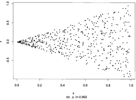
The following Figure 3.1 and Table 3.1 illustrate the behaviour of with a simulated

conical data set of 500 observations.

The observations are heteroscedastic and have mean zero. The correlation between x and y is ;0:002. In Table 3.1 empirical -values for dierent are exhibited. They are

calculated by replacing in (3.5) q(xt) by its kernel estimator qn;(xt) and q by the

empirical unconditional quantile of the rst t;1 data values z

1;:::;zt;1. The latter can

be interpreted as a naive forecast of q(xt).

The ndings of Abberger (1996, 1997) for several German stock returns were -values

close to zero for the median and increasing in a U-shaped form towards the boundary areas around = 0:01 respectively = 0:99.

ARCH- and GARCH models represent a very specic kind of parametric modeling for stu-dying the phenomenon of volatility.A exible alternative to the combination of an

ARMA-Table 3.1

0.01 0.05 0.10 0.25 0.50 0.75 0.90 0.95 0.99 0.43 0.36 0.27 0.10 0.01 0.11 0.26 0.34 0.41

model with ARCH- or GARCH-residuals is given by the

c

h

a

r

n

3 KERNELESTIMATIONIN TIME SERIES 11

Figure 3.1.

zt=m(xt) +(xt)t; (3.7)

studied by Hardle and Yang (1996) or Hardle, Tsybakov and Yang (1997). Here xt =

(zt;1;:::;zt;p)

0 is again the autoregressive vector (3.1),

t is a random variable with

mean zero and variance one. 2(x) is called the volatilityfunction. Given an estimator

for m , e. g. the NW-estimator mn according to (3.3), it was suggested that 2(x) can

be estimated by 2 n(xt) =gn(xt);m 2 n(xt); (3.8) where gn(x) = n P t=1 K xt;x h z2 t n P t=1 K xt;x h = n X t=1 z2 twn;t(x): (3.9)

Since the estimator (3.8) is based on a dierence, it can happen that from time to time a negative variance estimator results. This can be avoided if the volatility function is estima-ted on the basis of residuals. See (7.10), the discussion there and Feng and Heiler (1998a).

3 KERNELESTIMATIONIN TIME SERIES 12

In the context of time series analysis not only past values of the time series itself or of related series may occur as regressor variables, but also the time index itself, in which case xt = t , or some functions of the time index like polynomials or trigonometric functions.

This leads to smoothing approaches. In the case m(xt) = m(t) the NW estimator at

t consists in a weighted mean of the time series values in a neighbourhood [t;h;t+h] of

zt with nonrandom weights. Polynomials and trigonometric functions in t are used in

decomposing a seasonal time series into trend- cyclical and seasonal components according to an unobserved components model. This application will be studied in section 8 after the discussion of locally weighted regression.

In the area of quantile estimation the regressor xt = t leads to quantile smoothing.

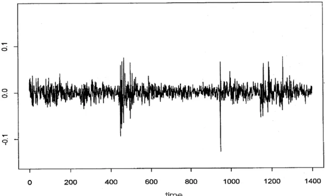
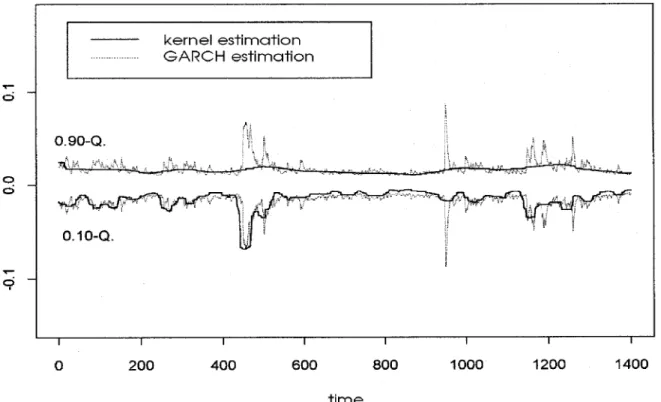
This technique was used by Abberger (1996, 1997) in order to compare the results of a nonparametric procedure for stock returns with those of a GARCH-model, evalua-ted with an S{Plus package under the standard assumption of an underlying Gaussi-an distribution. As Gaussi-an example we take daily discrete DAX returns, dened as zt =

(pricet;pricet

;1)=pricet;1, exhibited in Figure 3.2.

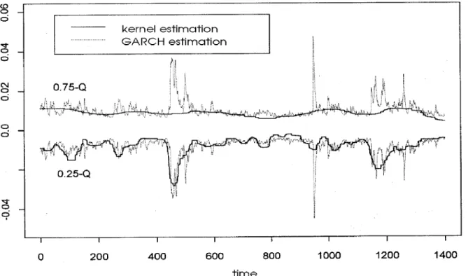
Since the Gaussian distribution is completely determined by mean and variance, conditio-nal quantiles can easily be calculated from the outcomes of the GARCH model estimation. The results are depicted in Figure 3.3 and 3.4 for the lower and upper quartiles and for the 0:1 and 0:9 quantiles, respectively. Two messages can be learned from the results. The rst is that the asymmetric behaviour of volatility, which is revealed by the nonparametric approach, will remain completely hidden by the choice of a wrong parametric model which is being oered as the default option by the package. In the presented example, which is not untypical for stock returns, volatility is a phenomenon which has mainly to do with movements in the lower tails of the conditional distributions. The second nding in the gures is that kernel smoothing is very robust towards aberrant and erratic observations in the course of the time series, whereas GARCH models react very sensitively to them.

3 KERNELESTIMATIONIN TIME SERIES 13

4 PROBLEMSOFSIMPLEKERNELESTIMATIONANDRESTRICTEDAPPROACHES14

Figure 3.3

4 Problems of simple kernel estimation and restricted

approaches

The nonparametric approaches we have treated so far suer from two drawbacks. One is the so-called "curse of dimensionality", the other is increased bias in cases of a highly-clustered design density and particularly at the boundaries of the x-space. Curse of dimen-sionality describes the fact that in higher dimensional regression problems the subspace of IR

p+1 spanned by the data is rather empty, i.e., there are only few observations in the

neighbourhood of a point x 2 IR

p _{. In practice this happens to be the case already for}

p > 2 .

Several proposals have been made to cope with the curse of dimensionality problem. We will describe only two of them very shortly. The rst consists in decomposing IR

p _{into a}

class of J disjoint course patterns, Aj;j = 1;:::;J with the aid of a non-hierarchical

cluster analysis. These J disjoint sets serve then as the states of a homogeneous Markov chain. In the model

4 PROBLEMSOFSIMPLEKERNELESTIMATIONANDRESTRICTEDAPPROACHES15

Figure 3.4

mn(xt) =N;1

j n

X

s=1

zs

1

where Nj is the number of course patterns of length p from the time series in Aj . Here

the estimator is an unweighted mean of all values following courses in pattern class Aj .

Markov chain models of this type were rst used by S. Yakowitz (1979b) for analysing time series of water runo in rivers. Asymptotic properties for this type of model are discussed by Collomb (1980, 1983).

Gouriroux and Montfort (1992) examined a corresponding model for economic time series by incorporating volatility. They called their model

zt=XJ j=1 j

1

1

a qualitative threshold ARCH model.

Another proposal in order to cope with the curse of dimensionality is given by the so-called generalized additive models, studied by Hastie and Tibshirani (1990), which are dened

5 LOCALLY WEIGHTED REGRESSION 16 as zt=m0+ p X j=1 mj(zt;ij) +at:

The components mj are again of a general form. For estimation so-called backtting

al-gorithms such as the alternating conditional expectation algorithm (ACE) of Breiman and Friedman (1985) or the BRUTO algorithm of Hastie and Tibshirani (1990) may be used. The main idea of backtting goes as follows. In the above model E[zt;m

0 ;

P

j6=k

mj(zt;ij)] =

mk(zt;ik): Hence the variable in square brackets can be used to obtain a nonparametric

estimate for mk(zt;ik) . But of course, the other mj are unknown as well, so that the

estimation procedure has to be iterated until all the mn;j converge. For a more

detai-led study of generalized additive models the reader is refered to the book of Hastie and Tibshirani as well as to the two interesting papers by Chen and Tsay in JASA (1993). For further discussion and other approaches see also Hardle, Lutkepohl and Chen (1997). Quite a few proposals can be found in the literature dealing with the bias problem of NW-estimators close to the boundary and in cases of an unbalanced design in the x-space. Gasser and Muller (1979, 1984) suggested for the case p = 1 a system of variable weights, Gasser, Muller and Mammitzsch (1985) developed asymmetric boundary kernels and Mes-ser and Goldstein (1993) suggested variable kernels which automatically get deformed and thus reduce the bias in the boundary area.

Yang (1981) and Stute (1984) suggested a symmetrized k;NN estimator and Michels

(1992) proposed boundary kernels for bias reduction which can be carried over to the case p > 1 . We do not discuss the above mentioned proposals in more detail since the mentioned disadvantages can be repaired by using locally weighted regression.

5 Locally weighted regression

Locally weighted respectively local polynomial regression was introduced into the stati-stical literature by Stone (1977) and Cleveland (1979). The statistati-stical properties were investigated since then in papers by Tsybakov (1986), Fan (1993), Fan and Gijbels (1992, 1995), Ruppert and Wand (1994) and many others. A detailed description may be found in the book of Fan and Gijbels (1996).

For the sake of simplicity we start with the assumption that the regressor x is a scalar. For a better understanding we regard the data as being generated by a location-scale model

5 LOCALLY WEIGHTED REGRESSION 17

akin to the one considered in (3.7), where the are independent with E() = 0;V ar() = 1 and m(x0) =E(y

jx = x

0). m is assumed to be smooth in the sense that the (p+1)th

derivative exists at x0, so that it can be expanded in a Taylor series around x0 .

m(x) = m(x0) + (x ;x 0)m 0 (x0) +::: + (x ;x 0) rm(r)(x 0) r! + Rr(x) (5.2)

with the remainder term Rr(x) = (x;x 0) r+1 m(r+1) x0+(x ;x 0) =(r;1)!; 0 < < 1: (5.3) With j(x0) =m (j) (x0)=j!; j = 0;1;:::;r (5.4)

we arrive at a local polynomial representation for m, m(x) r X j=0 j(x0)(x ;x 0) j_{: (5.5)}

This approach motivates the nonparametric estimation of m as a local polynomial by solving the least squares problem

min2IR r+1 8 > < > : n X i=1 2 4y i; r X j=0 (xi;x)jj 3 5 2 K xi;x h 9 > = > ; :

With the design matrix Xx having the n rows [1;xi ;x;:::;(xi;x)r], the diagonal

weight matrix Wx = diag

K(xi;x

h )

and the vector y = (y1;:::;yn)

0 the solutions at x is given by ^(x) = (X0 xWxXx);1 X0 xWxy; (5.6)

and with ej being the j-th unit vector in IR

5 LOCALLY WEIGHTED REGRESSION 18 ^ m(x) = ^0 =e 0 1(X 0 xWxXx);1X0 xWxy; (5.7)

and that with ^ m(j)(x) = ^ j(x)j! = j!e0 j+1(XxWxXx) ;1X0 xWxy; j = 1;:::;r (5.8)

an estimator for the j-th derivative of m is given.

The case r = 0 yields the Nadaraya-Watson estimator (3.3). Let u = (rr(x1))ni

=1 be the residual vector containing the remainder terms according to

(5.3) at the data points. Then the conditional bias of ^(x) is given by B

^(x)

= (X0

xWxXx);1X0

xWxu;

and with x =W(x)2diag

2(x

i)

its conditional covariance matrix is V ar ^(x) = (X0 xWxXx);1(X0 xxXx)(X0 xWxXx);1:

The above two expressions cannot be used directly since they contain the unknown vector u of remainder terms and the unknown diagonal matrix x:

A rst order asymptotic expansion of the variance and the bias term uses the moments of K and K2 , denoted by

j =

Z

uj_{K(u)du and j =}Z

uj_K2(u)du;

which are contained in the matrices

S = (j+l)0j;lr; ~S = (j+l+1)0j;lr; S

= (

j;l)0j;lr

and the vectors cr = (r+1;:::2r+1); ~cr = (r+2;:::;2r+2): For an i. i. d.

sam-ple (y1;x1);:::;(yn;xn) with the marginal density f(x) > 0 and with f;m

5 LOCALLY WEIGHTED REGRESSION 19

2 continous in a neighbourhood of x we obtain for h

;! 0 and nhn ;! 1 the

asymptotic conditional variance V ar ^ m(j) (x) =e0 j+1S ;1 S S;1 ej+1 (j!)22(x) f(x)nh1+2j +op 1 nh1+2j : (5.9)

For the asymptotic conditional bias we have to distinguish between the cases where r;j is

odd and where r;j is even.

For r;j odd we have

Bias ^ m(j)(x) =e0 j+1S ;1c r_{(r + 1)!m}j! (r+1)(x)hr+1;j+o p(hr+1;j): (5.10)

For (r;j) even the asymptotic bias is

Bias ^ m(j)(x) =e0 j+1S ;1c~ r_{(r + 2)!}j! n m(r+2)(x) + (r + 2)m(r+1)(x)f 0(x) f(x) o hr+2;j+o p(hr+2;j); (5.11)

provided that f0 and m(r+2) are continuous in a neighbourhood of x and nh3

;!1: As

a very interesting fact we notice the dierence in asymptotic bias between r;j odd and

r;j even. For instance we have for the NW-estimator (r = 0;j = 0) ,

B(mn(x)) = h2[m00(x)=2 + m0f0(x)=f(x)]

2+op(h 2);

whereas for the local linear approach we obtain B(^m(x)) = h2m00(x)

2=2 + op(h 2):

We see that the bias of the local linear estimator has a simpler structure. The linear term in the bias expansion vanishes, whereas the expression for the variance is the same in both cases and given by 0

2(x)=nh: The bias of the NW-estimator does not only depend on

m0, but also on the score function ;f

0=f . This is the reason why an unbalanced design

leads to an increased bias.

5 LOCALLY WEIGHTED REGRESSION 20

estimating m it is sucient to consider r = 1 or r = 3; and for m0 only r = 2 or

r = 4 should be considered. In many applications r = j + 1 suces. Fitting a higher order polynomial will possibly reduce the bias, but on the other hand the variance will increase since more parameters have to be estimated locally.

If the regressor x is a vector rather than a scalar in most cases a local linear approach is chosen since in this case the step from r = 1 to r = 3 leads to strong increase of parameters to be estimated locally which entails an inacceptable increase in variance. Since ^j(x) = e0 j+1^ = e 0 j+1(X 0 xWxXx);1 X0 xWxy =Xn i=1 wj ni x i;x h yi (5.12)

for estimating j(x) = m(j)(x)=j! we have a similar expression as a weighted mean like for

the NW-estimator (3.3). The weights depend on the observations xi and on the location

of x in the design space.

It can be seen easily that the weights w_nij _{(ut) =wni}j

xi;xo

nh

satisfy the discrete moment conditions n X i=1 xi;x q wj ni x i;x h =jq with 0j;q r:

As a consequence of this the sample bias for estimating a polynomial with degree less than or equal to r is zero.

The variance of ^m(j)(x) is given by

V ar ^ m(j) (x) =Xn i=1 wj_nix i;x h 2 2 (xi):

The kernel with the weights w_nij _{(ut) is called theactive kernel.}

A rst order approximation to the wj_{ni is given if (X}0

xWxXx) is replaced by the kernel

moments matrix S . The according kernel

~K(j)(u) = e0

j+1S

5 LOCALLY WEIGHTED REGRESSION 21

is called the equivalent kernel. It satises the corresponding moment conditions

Z

uq~K(j)(u)du = _{jq 0}

j;q r: (5.14)

For instance, for the case r = 1;j = 0 we have ~K(u) = K(u); and for r = 2;j = 1 (esti-mation of m0) ~K(1)(u) =

;1

2 uK(u): This means that for estimating m itself in the

interior of the x-space the eective kernel is equal to the chosen symmetric kernel function itself whereas for estimating the rst derivative ~K(1) is a skew function. As a general

result ~K(j) is symmetric for j even and skew for j odd.

In terms of equivalent kernels the asymptotic conditional variance and the asymptotic conditional bias (for r;j odd) are

V ar ^ m(j)(x) = (j!)22(x) f(x)nh1+2j Z ~K(j)2(u)du + o p(nh;1;2j); (5.15) Bias ^ m(j)(x) = j!_{(r + 1)!m}(r+1)(x)hr+1;j Z ur+1 ~K(j)(u)du + o p(h;r;1+j): (5.16)

The big advantage of local polynomial regression over other smoothing methods consists in the automatic adaptation of the active resp. equivalent kernel to the estimation si-tuation in the boundary area. If x is scalar and x = min(xi);x

= max(x

i); then

for a given bandwith h the interior of the x-space is given by all observations in the interval h

x+h;x

;h i

: For all x in this interval the equivalent kernels ~K(j)

ha-ve the aboha-ve mentioned symmetry resp. asymmetry property. In the left boundary part

h

x;x+h i

the number of left neighbours in a local neighbourhood of a point x will be small compared to the numberof right neighbours and for x = x we have only right

neigh-bours. Corresponding considerations hold for the right boundary part h

x ;h;x i : For x2IR

p_{;(p > 1) the boundary area will often cover an important part of the whole design}

space. For (r ;j) odd the active resp. equivalent kernels automatically adapt to the

skew data situation in the boundary area. The situation in the right boundary area is illustrated in Figure 5.1 for the Epanechnikov kernel K(u) = 3

4(1 ;u

2)

+ for a local

li-near estimation of m (r = 1;j = 0) and a local quadratic estimation of m0(r = 2;j = 1):

We see how the weighting systems get deformed towards the boundary. The pictures for the left boundary area are symmetric to those in Figure 5.1. Since the size of the local neighbourhood shrinks towards the boundary the bias part of the mean squared error (MSE) will be lower in the boundary area than in the interior. On the other hand the variance part will increase since less observations are included in the local estimation and

5 LOCALLY WEIGHTED REGRESSION 22

Figure 5.1

;15 (dashes and points), at x

;6 (long dashes) and at the

boundary point x (solid line).

also due to the increasing deformation of the weighting system towards the boundary. Usually, the increase in variance overcompensates the reduction of the bias, particularly if m00 remains roughly the same in the boundary area. As a conseqence, the MSE will

increase towards the boundary. The increase will be even more pronounced for higher order polynomials.

For x 2 IR

p _{the local linear t is given as the solution of the least squares}

criteri-on n X i=1 h yi; 0 ; 0(x i;x) i 2 Kx i;x h ;

where K is a p{variate kernel. With the design matrix Xx with rows

1;(xi1 ;x 1);:::;(xip ;xp)

the solution has the same form as in (5.7).

Let K be a product kernel composed of the same univariate kernel and bandwidth h in each coordinate and let Hm(x) be the Hessian matrix of the second derivatives of m.

Then we get an asymptotic expression for the variance and the bias in the interior (see Ruppert and Wand, 1994)

V ar ^ m(x) = 0 2(x) f(x)nhp +op(nhp); (5.17)

5 LOCALLY WEIGHTED REGRESSION 23 and Bias ^ m(x) = h2 2 2tr fHm(x)g+op(ph 2): (5.18)

The above considerations about the advantage of a local linear approach compared to the local constant estimation, about its design adaptation property and its automatic boun-dary adaptation hold for the multivariate case in a similar way.

Up to now we considered local least squares regression to estimate the mean function m: But the idea of locally weighted regression turns out to be a very versatile tool for estimation in a variety of situations.

Yu and Jones (1998) consider the estimation of the conditional distribution function F(yjx): Let F

1(u) =

u

R ;1

K1(v)dv be the distribution function pertaining to a

sym-metric kernel density K1 and let h2 be a bandwidth. Yu and Jones consider a local

linear approach for F(yjx) which is motivated by the approximations

Eh F1(y ;y 0 h2 )jx 0 i F(y 0 jx 0) and F(y0 jx 0) F(y 0 jx) + _F(y 0 jx)(x;x 0) =0+ 0 1(x ;x 0); where _F(y0 jx) = @F(y 0 jx)=@x:

This suggests the least squares approach

n X i=1 h F1(y i;y h2 ); 0 ; 0(x i;x) i 2 K(xi;x h1 );

where K is a second kernel with bandwidth h1: The solution

~Fh1;h2(y jx) = ^ 0 =e 0 1(X 0 xWxXx);1X 0 xWxy~ (5.19) with ~y = F1( y1 ;y h2 );:::;F 1( yn;y h2 ) 0

is called alocal linear double-kernel smoothingby the authors. The estimator is continuous and has zero as left boundary value (for y;!;1)

and 1 as right boundary value. It can happen that the estimator ranges outside [0;1]: But this does not, as the authors say, give problems estimating q by

5 LOCALLY WEIGHTED REGRESSION 24

~

q(x) = ~F;1

h1;h2( jx):

This estimator involes the problem that two bandwidths h1 and h2 have to be chosen.

For a possible procedure with h2 < h1 we refer to the paper.

Fan, Yao and Tong (1996) considered a related idea for estimating the conditional density itself. E 1 h2 K1 y;y 0 h2 g(y 0 jx) + _g(y 0 jx)(x;x 0) = 0+ 0(x ;x 0)

with _g(yjx) = @g(yjx)=@x leads to the least squares criterion

n X i=1 1 h2 K1 yi;y h2 ; 0 ; 0(x ;x 0) 2 K xi;x h1 (5.20)

with the solution ^g(yjx) = ^

0 as in (5.19), where now the vector ~y is

~ y = 1h2 K1 y1 ;y h2 ;:::;K1 yn;y h2 0 :

The local constant approach leads to the traditional estimator (2.3). Fan, Yao and Tong also consider the case of a local quadratic approach for estimating the rst derivative. We will not pursue this case further here, since for the quadratic term p(p + 1)=2 more parameters have to be estimated.

In all local regression approaches so far we used the least squares criterion. Let us now look at cases were instead of the square function another convex loss function : IR !IR is

used which has a unique minimum at zero and let m(x) = argmin0E [(y

;

0) jx].

(u) = u2 yields the conditional expectation which we analyzed mostly so far. (u) = juj yields the conditional median. This is just a special case for = 1=2 of the loss

function (u) = juj+ (2;1)u, already mentioned in (3.6) . was introduced by

Koenker and Basset for parametric quantile estimation. The function 2(u) for various

5 LOCALLY WEIGHTED REGRESSION 25

Figure 5.2

In robustness considerations -functions were introduced which increase less rapidly than the square function and for which 0 is the so-called -function. See Huber (1981) or

Hampel et al (1986).

A local constant estimator for m is

^ m(x) = argmin0 n X i=1 (yi; 0)K(x i;x h ):

The known drawbacks of a local constant approach is that it cannot adapt to unbalanced design situations and that it has adverse boundary eects which require boundary correc-tions.

This idea leads to the estimator ^ m(x) = ^0 where ( ^0; ^) = argmin 0; n X i=1 yi; 0 ; 0(x ;x 0) Kx ;x 0 h : (5.21)

6 APPLICATIONS OF LOCALLY WEIGHTED REGRESSION TO TIME SERIES26

For a -function belonging to a robustness class, such as Huber's M-type estimators known methods for robust estimation can be applied in order to solve the minimum problem (5.21). We would like to remark that the use of kernels automatically safeguards against large deviations in the design space. For nonparametric robust M-, L- and R-estimation in a time series setting see Michels (1992).

For a local -quantile regression with the function (3.6) the local solution in (5.18)

can be evaluated by solving a linear programming problem, as was shown in the paper of Koenker and Basset (1978). An algorithm for evaluating this can be found in Koenker and Dorey (1987).

For the case of a general convex -function and i. i. d. observations asymptotic normality is proved in Fan, Hu and Truong (1994). The -quantile estimation according to (5.21) is also considered by Yu and Jones (1998) and compared with the estimator (5.19). For reasons of practical performance the authors prefer the double smoothing approach (5.19). They also give an asymptotic expression for the mean squared error for x scalar, which for the solution of (5.21) is given by

MSE ^ q(x) = Bias2 ^ q(x) +V ar ^ q(x) = 14h42 2q 00 (x) + 0(1 ;) nhf(x)f(q(x)jx) 2:

These expressions are used for suggestions of bandwidth choice.

The cases of robust locally linear regression and of quantile regression are also considered in Fan and Gijbels (1996).

6 Applications of locally weighted regression to time

series

Local linear or higher order polynomial regression, originally mainly considered for inde-pendent data, can be applied in the same way to stationary processes with certain memory restrictions. The reasons are the same as those mentioned at the beginning of section 3. Given two (dependent) random variables xs and xt and a point x in the design space,

the random variables 1

hK(xs;x

h ) and 1

hK(xt;x

h ) are nearly uncorrelated as h! 0. This is

the whitening by windowing principle and it is worthwile mentionening that this property

is not shared by parametric estimators. To handle memory restrictions in the proofs of consistency and asymptotic normality mixing conditions (strong mixing, uniform mixing or -mixing) are used. They give a bound to the maximal dependence between events being at least k instants apart from each other. Short term dependence does not have

6 APPLICATIONS OF LOCALLY WEIGHTED REGRESSION TO TIME SERIES27

much eect on local regression. But local polynomial techniques are also applicable under weak dependence in medium or long term. If suitable mixing conditions are fullled, local polynomial estimators for dependent data have the same asymptotic properties as for in-dependent data. Of course the bias is not inuenced by dependence, whereas the variance terms are aected. In proving asymptotic equivalence then the task consists in showing that the additional terms due to nonvanishing covariances between the variables are of smaller order asymptotically.

For a local linear estimation of m(x) = m(x1;:::;xp) in the autoregressive model (3.2)

the design matrix and the vectory have the form Xx = 0 B B @ zp;x 1; ::: z1 ;xp ... zn;1 ;x 1; ::: zn;p ;xp 1 C C A; y = 0 B B @ zp+1 ... zt;1 1 C C A; and with (xt;x) 0 = (z t;1 ;x 1;:::;zt;p ;xp)

0the esimator can be evaluated as in (5.7).

For x = xn+1 = (zn;:::;zn;p+1) 0,

^

m(xn+1) = ^0

yields the one-step ahead predictor. A direct k-step ahead predictor is given if y = (zp+k;:::;zn)

0 and if the last row of the X

x-matrix is (zn;k

;zn;:::;zn ;k;p+1

;zn ;p+1).

But in this case a succession of one-step ahead predictions seems preferable, as already mentioned in section 3.

Asymptotic normality results for locally linear autoregression can be found in Hardle, Tsybakov an Yang (1997) and in Fan and Gijbels (1996).

For the CHARN model zt = m(xt) +(xt)t the function g(xt) according to (3.9)

can be estimated in a similar way as above, where only in the vector y the time series values are replaced by the squares. Asymptotic normality for this case is shown in Hardle and Tsybakov (1997). For a residual based estimator of 2(x) see (7.10) or Feng and

Heiler (1998a).

The local linear estimation of a conditional density in a time series setting with the before mentioned double smoothing procedure as in (5.19) is considered in Fan, Yao, and Tong (1996) and in Fan and Gijbels (1996), where also asymptotic results can be found. For the estimation of of the conditional distribution function according to the propo-sal of Yu and Jones (1998) as in (5.19) and for a general solution of (5.21) asymptotic

7 PARAMETER SELECTION 28

results are known for independent data. See the papers of Yu and Jones (1998), Hardle and Gasser (1984) and Tsybakov (1986). For dependent data, we have not found yet formally puplished proofs. But considering the whitening by windowing eect makes it clear that for these cases consistently results will hold under suitable mixing conditions.

7 Parameter selection

One of the rst questions to be answered in the application of kernel smoothing is which type of kernel to use for dierent choices of r and j. It is well known that for r;j odd

in the interior of the x-space the Epanecknikov kernel K(u) = 3 4(1

;u 2)

+ is the one

which minimizes the mean squared error in the class of all nonnegative, symmetric and Lipschitz continuous functions and that for the endpoints x and x

the triangular

kernels (1;u)

1

[0;1](u) resp. (1+u)

1

area optimal solutions are not known.

It is easy to see that when looking at variance only the uniform kernel 1 2

1

[;1;1](u) is the

one minimizing the variance.

It is well known that in practice the choice of the kernel is not very important compa-red to the choice of the bandwidth. The Epanecknikov kernel will therefore be a good choice in many cases. Nonetheless in practice often higher oder kernels like the Bisquare or the Triweight are prefered. This has to do with the degree of smoothness, since the kernel estimates inherit the smoothness properties of the kernel. According to the degree of smoothness as introduced by Muller (1984), the uniform kernel has degree zero (not continuous), the triangle and the Epanecknikov kernel have degree 1 (continuous, but rst derivate not continuous), the Bisquare and the Triweight have degrees 2 and 3, respective-ly, and the Gaussion kernel has degree 1.

The most crucial task in kernel smoothing is bandwidth selection. Much ink has been spoiled on papers concerning this problem. It is hence impossible to give a comprehensive survey here. Instead we will discuss only a few basic ideas. The aim is to choose band-widths such that the conditional mean squared error, given by

MSE( ^m(j)(x)) = Bias2(^m(j)(x)) + V ar(^m(j)(x)) (7.1)

becomes minimal. We have to distinguish between a locally optimal banwidth and a glo-bally optimal, constant banwidth.

It is clear that a large bandwidth will lead to a low variance, but a high bias. Decreasing the bandwidth will increase the variance, but reduce the bias. An optimal bandwidth is

7 PARAMETER SELECTION 29

achieved when the changes in bias and variance balance.

Using the asymptotic expressions (5.15) and (5.16) for the conditional variance and bias, then minimizing (7.1) with respect to h yields for the (asymptotically) optimal band-width at x for a scalar x

h n=Cr;j(K) " 2(x) (m(r+1)(x))2f(x) 1 n # 1=(2r+3) ; (7.2)

where the constant Cr;j(K) = 2 6 4 ((r + 1)!)2 (2j + 1)R ~K(j)(u)2du 2(r + 1;j) n R ur+1~K(j)(u)du o 2 3 7 5 1=(2r+3) (7.3) depends only on r;j and the used kernel and can be calculated beforehand.

In time series applications we are mainly interested in a constant, global bandwidth, for which the integrated mean squared error (IMSE)

Z h

Bias(^m(j)(x))2+V ar(^m(j)(x)) i

w(x)dx

is chosen as criterion, where w is a weight function going to zero at the bounderies to avoid boundery eects. Minimizing the IMSE with respect to h yields the optimal global bandwidth h n=Cr;j(K) 2 4 R 2 (x) f(x)w(x)dx R fm (r+1)(x) g 2 w(x)dx 1 n 3 5 1=(2r+3) : (7.4)

For local linear estimation of m when x is a p-vector and the same bandwidth is chosen in each coordinate a similar expression can be derived (see Feng and Heiler, 1998a). Here

h n=c0 p n 1 (p+4) where

7 PARAMETER SELECTION 30 c0 = " 0 2 2 2(x) f(x)trfHm(x)g # 1 (p+4)

and Hm(x) is the matrix of second derivatives of m. All these expressions contain

quan-tities which are unknown and are therefore not amenable in practice. So called plug-in

techniques substitute these quantities by pilot estimates. For more details see Ruppert,

Sheather and Wand (1995).

A simple procedure of bandwidth selection for independent data, rstly developed to nd the smoothing parameter in spline smoothing, is cross validation. Let ^mh;i(xi) be the

so-called leave one out estimator of m at xi, where the observation (yi;xi) is not

used in the estimation procedure. Then the criterion is CV (h) = n;1 n X i=1 [yi;m^h;i(xi)] 2 (7.5) and hCV = argmin CV (h) is the cross validation bandwidth selector. The idea can

also be used for x 2 IR

p _{and for estimating derivatives. See Hardle (1990) for details.}

It can be shown that it converges almost shurely to the IMSE optimal bandwidth, but the convergence rate is with n;1=10 very low. The cross validation idea was

deve-loped for independent data. In a time series setting it is suggested to replace the leave one out estimator by a "leave block out" estimator, where for estimating at xi not only

the ith _{observation is omitted, but a whole block of data around (yi;xi). This idea was}

used by Abberger (1995, 1996) in smoothing the conditional -quantile, where the square function is replaced by the -function (3.6).

Let 2 be the variance of the residuals in an i.i.d. sample and in the time series case the

unconditional variance of the stationary process. Rice (1983, 1984) proposed a criterion R which for a general linear smoother is given by

R(h) = RSS(h);^ 2+ 2^2n;1 n X i=1 wni(xi); (7.6)

where the wni are the actual weights for estimating m(xi), ^2 is an estimate for 2 and

RSS(h) = n;1 n X i=1 [yi;m^h(xi)] 2 (7.7)

7 PARAMETER SELECTION 31

is the mean residual sum of squares. Under the assumption that ^2 is a consistent

estimator Rice (1984) showed that the proposed estimator hR =argmin R(h) is

asym-ptotically optimal in the sense that (hR;h 0)=h0

! 0 in probability, where h

0 is the

minimizer of the mean averaged squared error MASE(h) = n;1E ( n X i=1 [^mh(xi);m(xi)] 2 ) :

The rate of convergences of hR is the same low rate n;1=10 as for the cross validation

solution hCV. The main dierences between the two is that R involves an estimate of

2, whereas CV does not.

For ^2 Rice proposed an estimator based on rst dierences, whereas Gasser et al. (1986)

suggested to take second dierences (since they annihilate a local linear mean value func-tion), ^ 2 G= _3(n2 ;2) n;2 X i=1 yi+1 ; 1 2(yi+yi+2) 2 : (7.8)

An estimator based on a general difference sequence Dm =fd

0;d1;:::;dm g such that Pm 0 dj = 0 and Pm 0 d 2

j = 1 was considered by Hall et al. (1990) . The variance estimator

based on Dm is then ^ 2 m = (n;m) ;1 n;m X i=1 0 @ m X j=0 djyj+i 1 A 2 : (7.9)

Fan and Gijbels (1995) suggest the residual sum ofsquares criterion (RSC), which is based on a local estimator of the conditional variance derived under a local homogeneity assumption, ^ 2(x) = n P i=1 (yi;y^i) 2K xi;x h tr[Wx;Wx(X 0 xWxXx);1X0 xWx]: (7.10)

With this the RSC is dened as

7 PARAMETER SELECTION 32

where V is the rst diagonal elementof the matrix (X0

xWxXx);1(X0

xW2

xXx)(X0

xWxXx);1:

V;1 reects the eective number of local data points. RSC admits the following

in-terpretation. If h is too large, then the bias is large and hence also ^2(x). When the

bandwidth is too small, then V will be large. Therefore RSC protects against extreme choices of h.

The minimizer of E[RSC(x;h)] can be approximated by hn0(x) = " a0 2(x) 2Cr2 r+1nf(x) # 1=(2r+3) ; (7.12)

where a0 denotes the rst diagonal element of the matrix S

;1SS;1, i.e. a 0 = R ~K2(u)du and C r = 2r+2 ; c 0 rS;1c

r with the denitions given in section 5 and

r+1 = m

(r+1)(x)=(r + 1)!. h

n0(x) diers from the optimal bandwidth in (7.3) by an

adjusting constant which only depends on r;j, and the kernel used. Hence the latter one can be evaluated, h n(x) = Adj;rhn0(x); (7.13) where Adj;r = 2 6 4 (2j + 1)CrR ( ~K(j)(u))2du (r + 1;j) n R ur+1~K(j)(u)du o 2R ~K(u)2du 3 7 5 1=(2r+3) :

For the Epanechnikov and the Gaussian kernel these constants are tabulated for various r and j in Fan and Gijbels (1996).

For a global bandwidth the minimizer ^h of the integrated RSC, IRSC(h) =Z

RSC(x;h)dx

is taken, which in practice breaks down to evaluating a mean over certain grid points xi1;:::;xim. ^h is also selected from among a number of grid points in an interval

7 PARAMETER SELECTION 33

^hj;r =Adj;r^h: (7.14)

The RS criterion suers also from having a low convergence rate. Therefore the fol-lowing rened bandwidth selection procedure is suggested. It is a double smoothing (DS) procedure. The pilot smoothing consists in tting a polynomial of order r + 2 and se-lecting ^hj;r as above . With the bandwidth ^hr+1;r+2 estimates of ^r+1; ^r+2 and

^

2(x) are evaluated. With these pilot estimates in a second stage the d

MSE(j;r)(x;h) = d

Bias2

j;r(x) +V ard

j;r(x) is evaluated, where Biasd

j;r(x) denotes the (j + 1)th element of

the estimated bias vector and V ard

(j;r)(x) is the (j +1)

th _{diagonal element of the matrix}

(X0 xWxXx);1(X0 xW2 xXx)(X0 xWxXx);1^2(x). With S n;l = Pn i=1 K xi;x h (xi ;x)l the bias vector is estimated by ^br(x) = (X0 xWxXx);1 0 B B @ ^r+1Sn;r+1 + ^r+2Sn;r+2 ... ^r+1Sn;2r+1 + ^r+2Sn;2r+2 1 C C A:

In order to avoid collinearity eects it is suggested to modify the vector on the right side by putting Sn;r+3 =::: = Sn;2r+2 = 0, which yields

^br(x) = (X0 xWxXx);1 0 B B B B B B B B @ ^r+1Sn;r+1 + ^r+2Sn;r+2 ^r+1Sn;r+2 0 ... 0 1 C C C C C C C C A :

The global rened bandwidth selector is then given by the minimizer ^hRj;r of

Z

^

MSEj;r(x;h)dx: (7.15)

This rened technique leads to an important improvement over the RSC bandwidth selector.

For a balanced design, i.e. for equally spaced x values, Heiler and Feng (1998) propose a simple double smoothing procedure, where in the pilot estimation step the R-criterion

7 PARAMETER SELECTION 34

is used. In Feng and Heiler (1998b) a further improvement of this proposal can be found, where a variance estimator based on the bootstrap idea is used. Equally spaced x va-lues are for instance given in a time series setting where the regressor is the time index or a function of the timeindex. This kind of smoothing will be discussed in the next section. For order selection in a time series autoregression model with xt = (zt;1;:::;zt;p) and

^

mt(x) being the leave one out estimator according to (5.7), Cheng and Tong (1992) use

the cross validation criterion CV (p) = (n;r + 1) ;1 X t [zt;m^t(xt)] 2w(x t): (7.16)

where w is a weight function to avoid boundary eects.

Due to the curse of dimensionality problem it may be advisable not to take all lagged values zt;1;:::;zt;p into account but to look for a subset of lagged values which yields

the best forecasts. For a lag constellation xt(i) = (zt;i

1;:::;zt ;ip)

0 Tistheim and

Aue-stad (1994) propose to use the nal prediction error FPE(xt(i)) = n;1 X t [zt ;m(x^ t(i))] 2 f(i); (7.17)

where the factor

f(i) = 1 + (nhp);1 0bp(i) 1;(nhp) ;1[2Kp(o) ;po]bp(i); and o = Z K2(u)du; b p(i) = n;1 Xw 2(x t(i)) ^f(xt(i)) ;

^f(xt(i)) being a multivariate kernel density estimator. FPE in (7.16) is essentually a

sum of squares of one-step ahead prediction errors multiplied with a factor that penalizes small bandwidths and a large order p.

8 TIMESERIESDECOMPOSITIONWITHLOCALLYWEIGHTEDREGRESSION35

8 Time series decomposition with locally weighted

regression

As already mentioned in section 3, if xt is the time index itself or a polynomial in t,

then we arrive at trend smoothing. In a simple trend model zt=m(t) + at

the considerations at the beginning of section 5 deliver an estimator of the smooth trend function or its derivatives. Now the matrix Xt has the rows (1;s;t;:::;(s;t)r) for

s = 1;:::;n and Wt = diag(K(s;t

h )) . As an interesting fact one can easily see that in

the interior of the time series, i.e. for h tn;h the weights given in (5.8),

w_ntj _{(s) = e}0 j+1(X 0 tWtXt);1(1;s ;t;:::;(s;t) r_)K s;t h ; are shift invariant in the sense wj

n;t+1(s + 1) = wjnt(s) . This means that in the interior of

the time series the local polynomial t works like a moving average. But the big advantage over other trend smoothing techniques lies in the automatic boundary adaptation of the procedure. This property makes the idea of extending the local regression approach to so-called unobserved components models very appealing.

Nonparametric estimation of trend-cyclical movements and of seasonal variations and their separation by local regression represents an interesting alternative to procedures based on parametric models like X{12 or TRAMO{SEATS. These involve extrapolation methods on either end of the time series in order to be able to estimate the components also in the boundary parts of a time series. This can lead to serious problems if unusual observations in the end parts of time series yield grossly erroneous forecasts. The latter problem will not appear with a local regression approach. Note also that with a data driven parameter selection the procedure works in a fully automatic way.

The decomposition of a time series into trend{cyclical and seasonal components by LOcally WEighted Scatterplot Smoothing (LOWESS) was suggested by Cleveland et al. (1990). The procedure discussed here is dierent from their procedure in essential features. We consider the additive (unobserved) components model

8 TIMESERIESDECOMPOSITIONWITHLOCALLYWEIGHTEDREGRESSION36

For the sake of simplicity we assume that fatg is a white noise sequence with mean zero

and constant variance 2. T(t) represents the trend cyclical and S(t) the seasonal

component. The usual assumption with respect to T is that it has certain smoothness properties so that the considerations at the beginning of section 5 apply, leading to a local polynomial representation of order r. With respect to the seasonal variations the usual assumption is that they show a similar pattern from one seasonal period to the next, but they are allowed to vary slowly in the course of time. Hence a natural assumption is that they can locally be approximated by a Fourier series, containing the seasonal frequency and its harmonics,

S(s) =Xq

j=1

[j(t)cos2j(s;t) + j(t)sin2j(s;t)]; (8.2)

where is the seasonal frequency, = 1=P and P is the period of the season. Of course q 1=2 (and for q = 1=2 the last sine term has to be omitted).

Let

ut(s) = (cos2(s;t);sin2(s;t);:::;cos2q(s;t);sin2q(s;t)) 0 ; (t) = (1(t);1(t);:::;q(t);q(t)) 0 : Then S(s) = (t)0u t(s).

With the local polynomial representation for the trend-cyclical part T(s) =Xr j=0 j(t)(s;t) j _=(t)0x t(s); where (t) = (0(t);:::;r(t)) 0 ; xt(s) = (1;s;t;:::;(s;t)r) 0

, the local least squares criterion is n X s=1 [zt;(t) 0x t(s);(t) 0u t(s)]2 K s;t h : (8.3)

With the design matrices X1t with rows xt(s) 0, X

2t with rows ut(s) 0, X

t = (X1t...X2t), the

composed vector (t)0 = ((t)0;(t)0) and the weight matrix W

t=diag K s;t h the solution is

8 TIMESERIESDECOMPOSITIONWITHLOCALLYWEIGHTEDREGRESSION37 ^ (t) = (X0 tWtXt);1 X0 tWty (8.4) ^T(t) = e0 1(X 0 tWtXt);1 X0 tWty (8.5) ^S(t) = (o0 ;0 s)(X0 tWtXt);1 X0 tWty; (8.6)

where o0 is a row of zeroes of length r + 1 and 0

s is a row vector of length 2q with

entries 0

s= (1 0 1 0:::1 0). It picks out the ^j(t), pertaining to the cosine terms in ^S(t).

The estimator for the jth _{derivative T}(j) of T is

^T(j) = j!e0 j+1(X 0 tWtXt);1 X0 tWty: (8.7)

All the above estimators work as moving averages in the interior part of the time series and have for r;j odd the simple boundary adaptation property discussed in section 5.

The decomposition ^m(t) = ^T(t) + ^S(t) is not unique, since the matrix X0

tWtXt is

not block diagonal. This could of course be achieved by an orthogonalization procedure but seems not to be compelling for practical purposes. We call the above decompostion a

natural decomposition.

For parameter selection rst a decision has to be made about the degree of the trend polynomial T and the trigonometric polynomial S. Since the seasonal variations are involved in the local approach the bandwidths should be such that at least three to ve periods of the season are included. In order to achieve this, the modelization of T should be rather exible. Hence for the interior part of the time series the polynomial degree r = 3 may be preferable to the choice r = 1. A data driven choice for a joint selecti-on of r and bandwidth h is a very dicult task since the two parameters are highly correlated. A higher r allows a larger bandwidth and vice versa. In our experience col-lected so far a data driven procedure for the interior part always opted for the highest allowed degree rmax that was put beforehand even if the MSE criterion included a penalty

term for overparameterization. As far as the trigonometric polynomial is concerned, all harmonic terms should be included, unless an inspection of the periodogramme or the esti-mated spectrum reveals that one or even more of the seasonal frequences can be ommitted. After this preselection of parameters a procedure for bandwidth selection is needed. Since for an equidistant time series the "design density" f is a constant the procedure is so-mehow simpler than in the general situation discussed in section 7.

poly-8 TIMESERIESDECOMPOSITIONWITHLOCALLYWEIGHTEDREGRESSION38

nomial of degree r + 2 is tted and the bandwidth is selected with the Rice criterion with respect to ^m = ^T + ^S. But due to seasonal variations the dierence based varian-ce estimator (7.8) has to be altered. Heiler and Feng (1996) and Feng (1998) propose a seasonal dierence based variance estimator of the form in (7.9), where not only a local linear function, but also a local periodic function is allowed for.

An example for monthly data (P = 12) is D26;12=c

;1

f;1;2;;1;0;0;0;0;0;0;0;0;0;2;;4;2;0;0;0;0;0;0;0;0;0;;1;2;;1g;

where c is determined such that Pm

j=0

d2

j = 1:

D26;12 annihilates a local linear trend and a local periodic function with periodicity

P = 12. Similar sequences can easily be constructed. Let ^2

G be the resulting estimator and let g be the minimizer of the R-criterion(7.6).

With ^mg = ^Tg+ ^Sg the resulting estimator is denoted.

For an arbitrary h the weights wht(s) for estimating ^Th(t) + ^Sh(t) are the

com-ponents of the vector (1 0;:::;0;0

s)(X0

tWtXt);1

X0

tWt, where for Wt a kernel with

bandwidth h is taken.

Using the pilot estimates ^mg(t) the bias part of the MSE at t for an estimator with

bandwidth h is estimated by

d

Bias(^mh(t)) =Xn

s=1

wht(s)^mg(s);m^g(t)

which yields for the bias part of the mean averaged squared error MASE(h) B(h) = n;1 n X t=1 d Bias2 (^mh(t)) = n;1 n X t=1 ( n X s=1 wht(s)^mg(s);m^g(t) ) 2 : (8.8)

The variance is estimated by V (h) = n;1^2 n X t=1 n X s=1 wht(s)2; (8.9)

8 TIMESERIESDECOMPOSITIONWITHLOCALLYWEIGHTEDREGRESSION39

where ^2 should be a suitable root-n consistent estimator of ^2.

After the rst pilot step a minimizer ~h of the criterion

MASE(h) = B(h) + V (h) (8.10)

is evaluated over a grid, where in the second step the estimator ^2

G is used in V (h).

This second step leads already to a considerable improvement over the simple R-criterion, but the estimator ^2

G is still not very good. Hence an improved estimation with a lower

polynomial degree and a bandwith gv larger than g is proposed. For details see Feng

and Heiler (1998). According to considerations therein an estimator for gv can easily be

found by multiplying the minimizer ~h of (8.10) with a correction factor. This factor only depends on the used kernel and on the polynomial degree r, ^gv =CFr~h:

For instance, we get for the Epanechnikov kernel CF1 = 1:431, CF3 = 1:291, for the

Bi-square kernel CF1 = 1:451, CF3 = 1:300 and for the Gaussian kernel CF1= 1:489 and

CF3 = 1:305. See Table 5.1 in Muller (1988) or Table 1 in Feng and Heiler (1998).

Let now ^mgv = ^Tgv + ^Sgv be an estimator with bandwidth gv . Then an improved

variance estimator is obtained by taking the mean squared residuals ^ 2 B =n;1 n X t=1 [zt;m^gv(t)] 2 : (8.11)

In a third step this variance estimator is plugged into (8.9) for ^2 and with this again a

minimizer h of the MASE (8.10) is evaluated.

In principle this procedure can be iterated several times, where in the next step with a polynomial of degree r + 2 a new bias estimator is evaluated.

The above described procedure yields a bandwidth h for the interior part of the time

series, where after the selection of h the interior is given by [h+ 1;n ;h

]. As

descri-bed in section 5 the procedure automatically adapts towards the boundaries. But as also described there due to increasing variance the MSE will increase as well, particularly if r = 3 is chosen, as was recommended at the beginning of this section.

One possibility to at least partly compensate for that is to switch to a nearest neighbour estimator in the boundary area, that is, to keep the total bandwidth hT = 2h+1 constant

at both ends of the time series. This means that for estimating from t = n;h

+ 1 to

t = n the same local neighbourhood is used (and similarly for the left boundary).

8 TIMESERIESDECOMPOSITIONWITHLOCALLYWEIGHTEDREGRESSION40

approach (for T) may be recommended whenever the MSE for r = 1 becomes smaller than that for r = 3. In order to do that, for the given bandwidth and the asymmetric neighbourhood situation at each time point in the boundary area with the corresponding active weighting systems the MSE0s for r = 3 and r = 1 have to be evaluated according

to the procedure described above. As soon as MSE1 < MSE3, a local linear approach is

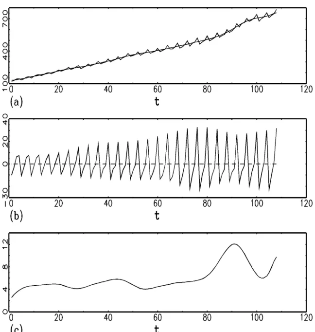
chosen forT and maintained to the end point. According to practical experiences collected so far such a switch happened to come to eect close to the end points in almost all cases. In Figures 8.1 and 8.2 we present two examples where the discussed decomposition proce-dure is applied. The rst time series is the quarterly series of the German GDP from 1968 to 1994. In the top panel in Figure 8.1 the time series itself and the estimated trend-cyclical component are exhibited. In the middle the estimated seasonal component is shown and in the bottom panel the rst derivative of the trend-cyclical is exhibited. This latter picture shows clearly the temporary boom after German reunication. The double smoothing pro-cedure with bootstrap variance estimator selected h = 11 as bandwidth. The polynomial degree was two for estimating the rst derivative and three for the other estimations. The second example presented in Figure 8.2 shows corresponding results for the monthly series of the German unemployment rates (in per cent) from January 1977 to April 1995. Here the selected bandwidth is h = 21. The polynomial degrees are the same as in the previous example.

Cleveland (1979) proposed an iterative robust locally weighted regression in a general regression context and in Cleveland et al. (1990) this idea is also used in time series decomposition. It can easily be adapted to the procedure discussed here, although in their proposal the subseries of equal weeks, month, quarters etc. are treated separately.

The idea consists in looking at the residuals rt=zt;m(t) of a rst, nonrobust procedure^

and to evaluate a robust scale measure for the residuals. Cleveland suggests to take the median of the jrtj. Since in many time series variability is dierent for dierent periods

within the season depending on the size of the seasonal component, it seems reasonable to evaluate dierent scale measures for the dierent periods of the season.

For t = 1;:::;n let j = h

t;1

P

i

+ 1 be the year index, j = 1::::;J = h

n;1

P

i

+ 1, where [:] denotes the integer part and let i = t;P(j;1) be the season index, i.e. zt;!zij.

Then for all i = 1;:::;P a robust scale measure i =medianj(jrijj)

is evaluated. From this so-called robustness weights are derived, which according to Cle-veland's proposal are given by

8 TIMESERIESDECOMPOSITIONWITHLOCALLYWEIGHTEDREGRESSION41

Figure 8.1

8 TIMESERIESDECOMPOSITIONWITHLOCALLYWEIGHTEDREGRESSION42

Figure 8.2

REFERENCES 43 ij =K rij 6i ;

where K is a kernel function (the bisquare kernel is being suggested).

In a second step the local estimation procedure is repeated, where the neighbourhood weights kst = K

s;t

h

in the diagonal weight matrices Wt are multiplied with the

corresponding robustness weights ij, where i and j are the season- and year index

cor-responding to s. Of course with the time dependent robustness weights the procedure is no more shift invariant, so that the least squares solution has to be evaluated for each t explicitely.

Starting with the new residuals the procedure can be iterated until the estimates stabilize. Since the robustness weights will change the active kernels, dierent bandwidths should be used in each iteration step. Cleveland (1979) claimed that two robust iterations should be adequate for almost all situations. In Feng (1998) with a stability criterion a higher number of iteration steps occured in most cases.

References

[1] ABBERGER, K. (1996).Nichtparametrische Schatzung bedingter Quantile in

Zeitrei-hen { Mit Anwendungen auf Finanzmarktdaten. Hartung-Gorre Verlag, Konstanz.

[2] ABBERGER, K. (1997). Quantile Smoothing in Financial Time Series. Statistical Papers, 38, 125{148.

[3] BONGARD, J. (1960). Some Remarks on Moving Averages. In: O.E.C.D. (editor), Seasonal Adjustment on Electronic Computers. Proceedings of an international con-ference held in Paris, 361-387.

[4] CHEN, R. (1996). A Nonparametric Multi-step Prediction Estimator in Markovian Structures. Statistica Sinica, 6, 603-615.

[5] CHEN, R. and TSAY, R.S. (1993). Functional-coecient Autoregressive Models.

Journal Amer. Statist. Assoc., 88, 298-308.

[6] CHEN, R. and TSAY, R.S. (1993). Nonlinear Additive ARX Models. Journal Amer. Statist. Assoc., 88, 955-967.

[7] CHENG, B. and TONG, H. (1992). On Consistent Non-parametric Order Determina-tion and Chaos (with discussion). Journal Royal Statist. Soc., Series B, 54, 427-474.