Iowa Geological Survey
Technical Information Series No. 49
Iowa Department of Natural Resources
Jeffrey R. Vonk, Director
April 2006
WALNUT CREEK WATERSHED RESTORATION
AND WATER QUALITY MONITORING PROJECT:
COVER
The Walnut Creek watershed is being restored to native tallgrass prairie from a landscape once dominated by row-crop agriculture. Currently, more than 3,000 acres of prairie have been planted by the U.S. Fish and Wild-life Service at the Neal Smith National WildWild-life Refuge in Jasper County.
WALNUT CREEK WATERSHED RESTORATION
AND WATER QUALITY MONITORING PROJECT:
FINAL REPORT
Iowa Geological Survey
Technical Information Series 49
Prepared by
K.E. Schilling
1, T. Hubbard
2, J. Luzier
2, J. Spooner
31Iowa Department of Natural Resources, Geological Survey 109 Trowbridge Hall, Iowa City, IA 52242-1319
2University of Iowa Hygienic Laboratory
University of Iowa; Oakdale Campus, Iowa City, IA 52242
3
NCSU Water Quality Group, North Carolina State University, Raleigh, NC 27695-7637
Supported, in part, through grants from the U.S. Environmental Protection Agency,
Region VII, Nonpoint Source Program
April 2006
Iowa Department of Natural Resources
Jeffrey R. Vonk, Director
TABLE OF CONTENTS
EXECUTIVE SUMMARY . . . xiii
INTRODUCTION . . . 1
Background . . . 1
Need for Project . . . 2
Walnut Creek Monitoring Project . . . 3
Project Objectives . . . 4
MONITORING PLAN DESIGN . . . 4
Study Area . . . 4
Monitoring Design . . . 6
METHODS . . . 8
Land Cover Tracking . . . 8
USGS Stream Gaging Stations . . . 9
Suspended Sediment . . . 9
Chemical Parameters . . . 9
Biomonitoring . . . 10
Statistical Methods . . . 10
Hydrograph Separation and Chemical Loads . . . 12
LAND RESTORATION IMPLEMENTATION . . . 12
Cropland Management Plan . . . 12
Herbicide and Fertilizer Management . . . 12
Land Use . . . 13
Nitrogen Application Reductions . . . 15
Pesticide Application Reductions . . . 17
HYDROLOGY . . . 18 Precipitation . . . 18 Discharge . . . 20 Trends . . . 25 Discussion . . . 27 SUSPENDED SEDIMENT . . . 33
Suspended Sediment Loads . . . 33
Suspended Sediment Concentrations . . . 36
Trends . . . 37
Discussion . . . 40
FIELD PARAMETER MEASUREMENTS . . . 46
ANIONS . . . 50
Nitrate Concentrations . . . 51
N-Cl Ratios . . . 54
Chemical Loads . . . 54
Trends . . . 56
Regression Model Development . . . 56
Final Multiple Linear Regression Model to Test for Changes Over Time . . . 59
Discussion . . . 61 HERBICIDES . . . 66 Concentrations . . . 66 Loads . . . 71 Trends . . . 72 Discussion . . . 73 FECAL COLIFORM . . . 76 Counts . . . 77 Trends . . . 78 Discussion . . . 79 PHOSPHORUS . . . 80 Trends . . . 82 Discussion . . . 83 BIOMONITORING . . . 84 Benthic Macroinvertebrates . . . 85 Fish . . . 87
Relation of FIBI to Reference Sites . . . 89
DISCUSSION. . . 92
Detecting Changes in Nitrate . . . 92
Detecting Changes in Runoff NPS Pollutants . . . .102
Detecting Changes in Biological Indices . . . .104
Detecting Changes in Suspended Sediment . . . .105
Sediment Erosion Model . . . .105
Sediment Sources . . . .106
Lag Time for Detecting Changes in Sediment Export . . . .109
LESSONS LEARNED . . . .111
CONCLUSIONS . . . .112
ACKNOWLEDGEMENTS . . . .115
LIST OF FIGURES
Figure 1. Location map including refuge ownership and future acquisitionboundaries. . . 3
Figure 2. Cross section of alluvium in Walnut Creek floodplain. . . 7
Figure 3. Sampling locations in Walnut Creek and Squaw Creek watersheds. . . 8
Figure 4. Land cover in 1990 and 2005 in the Walnut Creek and Squaw Creek watersheds. . . 14
Figure 5. Change in row crop land cover in the Walnut Creek and Squaw Creek watersheds from 1990 to 2005. . . 15
Figure 6. Annual and cumulative prairie plantings in Walnut Creek watershed. . . 16
Figure 7. Annual precipitation totals measured at project U.S.G.S. gages and Newton weather station. . . 18
Figure 8. Variations in monthly precipitation. . . 20
Figure 9. Average monthly precipitation during the project. . . 21
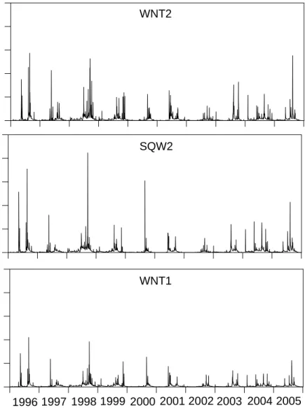
Figure 10. Daily discharge at WNT2, SQW2 and WNT1 at U.S.G.S. gaging stations. . . 22
Figure 11. Comparison of annual stream discharge characteristics at WNT2 and SQW2. . . 24
Figure 12. Time series of total monthly discharge at WNT2 and SQW2. (Solid line = total streamflow; dashed line = baseflow). . . 25
Figure 13. Relation of annual discharge at gaging sites to annual precipitation. . . 26
Figure 14. Response of Walnut Creek stage to precipitation in Water Year 2003. . . 27
Figure 15. Hydrograph of Walnut Creek discharge measured on May 8, 2003. . . 27
Figure 16. Box plots of total discharge by month at WNT2 and SQW2 gaging stations. Box plots illustrate the 25th, 50th and 75th percentiles; the whiskers indicate the 10th and 90th percentiles; and the circles represent data outliers. . . 27
Figure 17. Fraction of annual discharge and baseflow at WNT2 and SQW2 by month. . . 28
Figure 18. Ratio of precipitation to discharge at WNT2 and SQW2 by month. . . 28
Figure 19. Average discharge and baseflow at gaging sites by month. . . 29
Figure 20. Fraction of total monthly discharge as baseflow. . . 29
Figure 22. Time series of daily sediment loads measured at USGS gaging sites. . . 34
Figure 23. Cumulative sediment load and discharge at USGS gaging sites. . . 35
Figure 24. Time series of monthly sediment loads at WNT2 and SQW2. . . 36
Figure 25. Box plots of monthly sediment loads. . . 37
Figure 26. Relation of annual sediment yield to discharge at USGS gaging sites. . . 39
Figure 27. Box plots of suspended sediment concentrations by month at WNT2 and SQW2. . . 40
Figure 28. Relation of log daily discharge to log suspended sediment concentrations at USGS gaging sites. . . 40
Figure 29. Relation of log daily discharge to log suspended sediment concentrations by month at WNT2. . . 41
Figure 30. Relation of log daily discharge to log suspended sediment concentrations by month at SQW2. . . 42
Figure 31. Box plots of pH measured at Walnut and Squaw creek monitoring sites. . . 49
Figure 32. Box plots of specific conductance measured at Walnut and Squaw creek monitoring sites. . . 49
Figure 33. Box plots of specific conductance by month measured at Walnut and Squaw creek monitoring sites. . . 49
Figure 34. Box plots of dissolved oxygen measured at Walnut and Squaw creek monitoring sites. . . 50
Figure 35. Box plots of dissolved oxygen by month measured at WNT2 monitoring site. . . 50
Figure 36. Box plots of turbidity measured at Walnut and Squaw creek monitoring sites. . . 50
Figure 37. Box plots of turbidity by water year measured at WNT2 monitoring site. . . 51
Figure 38. Box plots of turbidity by month measured at WNT2 monitoring site. . . 51
Figure 39. Time series of nitrate concentrations measured at upstream/downstream sites in Walnut and Squaw creek watersheds. . . . 53
Figure 40. Relation of nitrate concentrations to discharge at WNT2 and SQW2. . . 54
Figure 41. Box plot of nitrate concentrations by water year at upstream/downstream sites in Walnut and Squaw creek watersheds. . . 55
Figure 42. Box plots of nitrate concentrations by water year at Squaw Creek subbasin sites. . . 56
Figure 43. Box plots of nitrate concentrations by water year at Walnut Creek
subbasin sites. . . 57
Figure 44. Box plots of nitrate concentrations by month at upstream/downstream
sites in Walnut and Squaw creek watersheds. . . 58
Figure 45. Time series of chloride concentrations measured at upstream/downstream
sites in Walnut and Squaw creek watersheds. . . 59
Figure 46. Time series of sulfate concentrations measured at upstream/downstream
sites in Walnut and Squaw creek watersheds. . . 60
Figure 47. Ratios of nitrate and chloride concentrations at upstream to downstream sites. . . . 61
Figure 48. Relation of annual nitrate, chloride and sulfate losses to annual discharge
at USGS gaging stations. . . 63
Figure 49. Box plots of monthly nitrate loads at WNT2 and SQW2. . . 64
Figure 50. Relation of nitrate concentrations at WNT2 to regression covariates. . . 66
Figure 51. Box plots of atrazine concentrations by water year at upstream downstream
sites in Walnut and Squaw creek watersheds. . . 70
Figure 52. Relation of atrazine concentrations to discharge at WNT2 and SQW2. . . 71
Figure 53. Box plots of atrazine concentrations by water year at Walnut Creek
subbasin sites. . . 72
Figure 54. Box plots of atrazine concentrations by water year at Squaw Creek
subbasin sites. . . 73
Figure 55. Detection frequency of cyanazine by water year at upstream and
downstream sites in Walnut and Squaw creek watersheds. . . 74
Figure 56. Box plots of monthly concentrations of atrazine, acetochlor and desethylatrazine at downstream monitoring sites (WNT2 and SQW2)
in Walnut and Squaw creek watersheds. . . 75
Figure 57. Box plots of atrazine loads by month at WNT2 and SQW2 monitoring sites. . . . 77
Figure 58. Box plots of desethylatrazine loads by month at WNT2 and SQW2
monitoring sites. . . 78
Figure 59. Annual atrazine and desethylatrazine loads estimated for various watershed
areas in Walnut and Squaw creek watersheds. . . 79
Figure 60. Box plots of fecal coliform concentrations by water year at upstream and downstream sites in Walnut and Squaw creek watersheds. A reference
line for 200 counts/100 ml is indicated. . . 83
Figure 61. Box plots of fecal coliform concentrations by water year at Walnut Creek
Figure 62. Box plots of fecal coliform concentrations by water year at Squaw
Creek subbasin sites. A reference line for 200 counts/100 ml is indicated. . . 85
Figure 63. Box plots of fecal coliform concentrations by month at upstream and downstream monitoring sites in Walnut and Squaw creek watersheds.
A reference line for 200 counts/100 ml is indicated. . . 86
Figure 64. Relation of fecal coliform concentrations to discharge at WNT2 and SQW2. . . . 87
Figure 65. Box plot of phosphorus concentrations by water year at upstream and
downstream sites in Walnut and Squaw creek watersheds. . . 90
Figure 66. Box plots of phosphorus concentrations by water year at Walnut and
Squaw creek subbasin sites. . . 91
Figure 67. Relation of phosphorus concentrations to discharge at WNT2 and SQW2. . . 92
Figure 68. Box plots of phosphorus concentrations by month at WNT2 and SQW2. . . 94
Figure 69. Box plots of annual benthic macroinvertebrate metrics in Walnut and
Squaw creek watersheds. . . 98
Figure 70. Summary of annual Walnut and Squaw creek IBI scores. . . 102
Figure 71. Relation of change in nitrate in stream nitrate concentrations (as determined by statistical methods) with change in percentage of land
cover in row crops in watersheds and subbasins. . . 104
Figure 72. Longitudinal profile of streambed elevation from stream gage sites WNT2
to WNT1 in Walnut Creek watershed. . . 108
LIST OF TABLES
Table 1. Basin characteristics of the Walnut and Squaw creek watersheds. . . 5
Table 2. Soil characteristics in the Walnut and Squaw creek watersheds. . . 6
Table 3. Summary of sampling locations, parameters and frequency. . . 10
Table 4. Summary of land cover in Walnut and Squaw creek watersheds
(1990 and 2005). . . 13
Table 5. Summary of annual precipitation totals (in inches) and departure from
long-term average for central Iowa (33.43 inches). . . 19
Table 6. Summary of annual discharge and baseflow values measured at WNT2, SQW2, WNT1 and WNT2-1 (WNT2-1 estimated by subtracting WNT1
from WNT2). . . 23
Table 7. Trend test for mean daily discharge at WNT2. Each month was allowed a different slope and intercept. Trends were adjusted for autocorrelation
Table 8. Trend test for mean daily discharge at WNT1 and SQW2. Each month was allowed a different slope and intercept. Trends were
adjusted for autocorrelation and covariates (as indicated). . . 31
Table 9. Summary of annual sediment loads and concentrations at WNT2,
SQW2 and WNT1. . . 32
Table 10. Percentage of annual sediment loads at WNT2, SQW2 and WNT1
from nonconsecutive 1-day, 5-day, 10-day and 20-day periods. . . 35
Table 11. Summary of average monthly sediment loads and concentrations at
WNT2, SQW2 and WNT1. . . 38
Table 12. Frequency of occurrence of various suspended sediment concentrations
for the 10-year monitoring period. . . 39
Table 13. Trend test for mean daily sediment concentrations and loads at WNT2. Each month was allowed a different slope and intercept. Trends were
adjusted for autocorrelation and covariates (as indicated). . . 43
Table 14. Trend test for mean daily sediment concentrations and loads at WNT2. Each month was allowed a different slope and intercept. Trends were
adjusted for autocorrelation and covariates (as indicated). . . 44
Table 15. Trend test for mean daily sediment concentrations and loads at WNT1 and SQW2. Each month was allowed a different slope and intercept.
Trends were adjusted for autocorrelation and covariates (as indicated). . . 45
Table 16. Summary of values for field parameters measured at 10 monitoring sites
for water years 1996 to 2005. . . 48
Table 17. Summary of mean annual nitrate, chloride and sulfate concentrations
at 10 project monitoring sites. . . 52
Table 18. Discharge and loss of anions, herbicides and phosphorus from various
watershed areas. . . 62
Table 19. Estimated flow-weighted concentrations of anions, herbicides and
phosphorus from various watershed areas. . . 65
Table 20. Trend tests for changes in nitrate concentrations over time at project
monitoring sites, adjusted for appropriate covariates as indicated. . . 67
Table 21. Estimated nitrate concentrations (mg/l) at project start (WY1996) and after 10 years (WY2005) for each month for downstream Walnut Creek station WNT2. Concentrations have been adjusted for the mean values of the covariates for each month and reflect estimated values from the
predictive regression multivariate models. . . 68
Table 22. Summary of herbicide detections and concentrations at project monitoring
Table 23. Summary of total annual atrazine export from various watershed areas. . . 76
Table 24. Percentage by month of average annual loss of atrazine and
desethylatrazine (DEA) from downstream WNT2 and SQW2 sites. . . 78
Table 25. Atrazine and desethylatrazine trends analysis results using MLE
regression for arbitrary censored data and seasonal Kendall tau. . . 80
Table 26. Atrazine and desethylatrazine trends analysis results at WNT2 using MLE regression for arbitrary censored data and covariates of date, log discharge, SQW2 concentrations and with or without upstream
WNT1 concentration as a covariate. . . 81
Table 27. Summary of fecal coliform concentrations at project monitoring sites
for water years 1996 to 2005. All concentrations in counts/100 ml. . . 82
Table 28. Summary of median annual fecal coliform counts at 10 project monitoring
sites. All concentrations in counts/100 ml. . . 86
Table 29. Trend tests for changes in fecal coliform concentrations over time at
project monitoring sites, adjusted for appropriate covariates as indicated. . . 88
Table 30. Summary of phosphorus concentrations at project monitoring sites. All
concentrations in mg/l. . . 89
Table 31. Summary of median annual phosphorus concentrations at 10 project
monitoring sites for water years 2000 to 2005. All concentrations in mg/l. . . 93
Table 32. Trend tests for changes in phosphorus concentrations over time at
project monitoring sites, adjusted for appropriate covariates as indicated. . . 95
Table 33. Description of benthic macroinvertebrate metrics. . . 96
Table 34. Description of metrics used to calculate the Index of Biotic Integrity
(IBI) for fish. . . 97
Table 35. Walnut Creek mean metric values-ANOVA between year comparisons
(years with no letters in common are significantly different). . . 99
Table 36. Data metric results (FIBI scores), unadjusted FIBI scores and adjusted
FIBI scores for Walnut Creek. . . 100
Table 37. Data metric results (FIBI scores), unadjusted FIBI scores and adjusted
FIBI scores for Squaw Creek. . . 101
Table 38. Mean score (0 to 10 possible) and 95% Confidence Interval (CI) for the Index of Biotic Integrity (FIBI) and 11 metrics scores for 10 reference sites (31 sampling events) and 12 randomly selected REMAP sites (12 sampling events) in Ecoregion 47F lacking stable riffles and
EXECUTIVE SUMMARY
The Walnut Creek Watershed Restoration and Water-Quality Monitoring Project was established in 1995 as a NPS monitoring program in conjunction with watershed habitat restoration and agricultural management changes implemented by the U.S. Fish and Wildlife Service (USFWS) at the Neal Smith National Wildlife Refuge and Prairie Learning Center (Refuge) in Jasper County Iowa. A large portion of the Walnut Creek watershed is being restored from row crop agriculture to native prairie and savanna. The objectives of the project were to: 1) perform comprehensive, long-term NPS monitoring in the Walnut and Squaw Creek watersheds; 2) quantitatively document over time reduction in NPS pollution and associated environmental improvements resulting from watershed habitat restoration and land management changes; and 3) use the monitoring data to increase our understanding of what implementation measures are successful and will be helpful in similar areas, and expand public awareness of the need for NPS pollution prevention measures in the State of Iowa.
The Walnut Creek Monitoring project utilized a paired-watershed as well as upstream/ downstream comparisons for analysis and tracking of trends. The Walnut Creek watershed is paired with the Squaw Creek watershed and a common basin divide is shared. Based on their similar basin characteristics, the watersheds are well suited to such a design. In addition, several subbasins are monitored in both watersheds to allow comparisons of differential implementation over time, and for analyzing their incremental contributions to the overall basin response. Four basic components comprised the project: 1) tracking of land cover and land management changes within the basins, 2) stream gaging for discharge and suspended sediment at two locations on Walnut Creek and one on Squaw Creek, 3) surface water quality monitoring in the Walnut and Squaw Creek watersheds, and 4) biomonitoring for aquatic macroinvertebrates and fish in Walnut and Squaw Creeks.
In 1990, land use in both Walnut and Squaw Creek watersheds was dominated by row crops of corn and soybeans, with 69.4 percent row crop in Walnut Creek and 71.4 percent in Squaw Creek. From 1990 to 2005, major changes in land cover occurred in both watersheds. Squaw Creek showed an increasing trend of row crop land use whereas row crop in Walnut Creek significantly decreased. In Squaw Creek, the 9.2 percent increase in row crop area from 1990 to 2005 was likely due to the passage of the Freedom to Farm Act in 1996 that appeared to have substantially increased row crop production. Lands previously categorized as grasslands enrolled in the Conservation Reserve Program (CRP) were converted to row crop production. This trend was particularly evident in subbasins SQW4 and SQW5 where the row crop percentage increased by 26 and 29 percent.
In Walnut Creek watershed, row crop land use decreased from 69.4 to 54.5 percent between 1992 to 2005 as a result of prairie restoration by the USFWS at the Neal Smith refuge. From 1992 to 2005, an average of approximately 222 acres of prairie were planted each year. As of 2005, 3,023 acres of land in Walnut Creek watershed were planted in native prairie, representing 23.5 percent of the watershed. In the subbasins, restored prairie accounted for 14.3 to 45.9 percent of the land area.
In Squaw Creek, nitrogen applications increased 12.8% over 1990 N applications whereas nitrogen applications in the Walnut Creek watershed decreased 21.4%. Pesticide applications in Walnut Creek watershed were reduced by nearly 28 percent compared to levels in 1990.
Hydrology and Suspended Sediment
Annual precipitation ranged from 25.4 to 41.57 inches at WNT2, 18.6 to 30.2 inches at WNT1 and 14.96 to 35.84 inches at SQW2. Stream discharge varied considerably from year to year with annual discharge varying more than 4-fold between water years 1996 to 2005. Annual discharge in Walnut Creek ranged from 4.31 inches in Water Year 2002 to 16.61 inches in Water Year 1998, whereas discharge in Squaw Creek SQW2) varied from 3.36 to 16.91 inches in the same two years. Average annual discharge for WNT2, SQW2 and WNT1 was similar for all gage sites, ranging between 8.62 to 8.93 inches. Streamflow in both watersheds was controlled in large part by seasonal precipitation patterns and soil moisture conditions, with greatest streamflow typically occurring during rainy periods when antecedent soil moisture conditions are high. During most years, this period included May and June when nearly one-half of the annual total streamflow typically occurred. Streamflow events were often characterized by flashy conditions typical of flow in incised channels. Few consistent patterns were evident in the statistical trends over time.
Suspended sediment concentrations and loads varied widely during the 10-year monitoring period. Total annual sediment export ranged from 3,706 to 18,367 tons in Walnut Creek and from 893 to 20,456 tons in Squaw Creek, with higher average annual loss higher in Walnut Creek (8,384 tons) than Squaw Creek (8,044 tons). Sediment transport through Walnut and Squaw creek watersheds was very flashy, evidenced by most of the annual suspended sediment load occurring during intermittent high flow events. While single day discharge events typically accounted for six to eight percent of the annual discharge, single day suspended sediment loads accounted for 25 to 37 percent of annual sediment total. A 20-day period in any given water year accounted for as much as 98 percent of the annual sediment total. This pattern of rapid conveyance of discharge and sediment loads is typical of incised channels. Greatest sediment transport typically occurred in May and June of each year, when on average these months accounted for 59.2 and 68.2% of the total annual load in Walnut and Squaw Creek watersheds, respectively. Annual sediment loss was slightly higher in Squaw Creek compared to Walnut Creek, averaging 0.69 and 0.65 tons/acre, respectively, with annual sediment yield significantly related to annual discharge.
Suspended sediment concentrations were similar in Walnut Creek and Squaw Creek, with average and median values of 104.1 and 46.0 mg/l at WNT2 and 90.1 and 42.7 mg/l at SQW2, respectively. Suspended sediment concentrations most commonly ranged between 20-50 mg/ l, with concentrations within this range approximately 35 to 39 percent of the time. Trends in daily sediment concentrations and loads were mixed and reflected the variable nature of sediment transport. One regression model indicated a decreasing trend in sediment concen-trations and loads over time was observed at WNT2 whereas another model indicated an increase over time.
Water Quality Monitoring
Nitrate concentrations have ranged between <0.5 to 14 mg/l at the Walnut Creek outlet (WNT2) and 2.1 to 15 mg/l at the downstream Squaw Creek outlet (SQW2). Mean nitrate concentrations were 1.7 mg/l higher at SQW2 than WNT2, and highest at the upstream monitoring sites in both watersheds, averaging 11.2 mg/l at WNT1 and 12.4 mg/l at SQW1.
Monthly nitrate concentrations exhibited clear seasonality, with higher concentrations occurring during May, June and July. Both Walnut and Squaw Creek watersheds have shown a similar temporal pattern of detection, with higher concentrations observed in the spring and early summer months coinciding with periods of application, greater precipitation and higher stream flow.
Total export of nitrate from Walnut Creek (WNT2) was lower than Squaw Creek (SQW2) averaging 22.0 and 26.1 kg/ha, respectively. The average flow-weighted concentration of nitrate was 8.6 mg/l in Squaw Creek and 10.4 mg/l in upper Walnut Creek but was 4.9 mg/l in lower Walnut Creek.
During the 10-year project, nitrate concentrations significantly decreased in Walnut Creek watershed, both at the watershed outlet and in monitored subbasins. At the Walnut Creek outlet (WNT2), the trend analysis indicated that nitrate concentrations decreased 0.119 mg/ l/year or 1.2 mg/l over 10 years when the Squaw Control watershed was utilized as a covariate. Nitrate concentrations decreased 3.4, 1.2 and 2.7 mg/l at WNT3, WNT5 and WNT6 subbasins, respectively. Nitrate concentrations increased 1.9 mg/l over 10 years in the downstream Squaw station SQW2 and 1.1 mg/l over 10 years in the upstream Squaw station SQW1. All subbasins in the Squaw Creek increased in nitrate concentrations, with subbasins SQW4 and SQW5 having quite dramatic increases. Over the 10-year monitoring program, nitrate in surface water in SQW4 and SQW5 subbasins increased 11.6 and 8.0 mg/l, respectively.
Atrazine and DEA were the most commonly detected herbicides in both watersheds with detection frequencies greater than 70 percent. Acetochlor was occasionally detected (up to 27 percent) whereas alachlor and metolachlor were rarely detectable (less than 5%). Cyanazine detections were also rare during the last five years of the project. Concentrations of atrazine often exceeded 1 ug/L during high streamflows in late spring/early summer; however, overall median concentrations of atrazine and DEA were less than 0.3 ug/l. May and June accounted for approximately 80 percent of the export load of atrazine, and the period of April through July accounted for 96 percent of the annual atrazine load. Statistical changes in herbicide concentrations over time were mixed, since both decreasing and increasing trends were observed. Sites WNT3 and SQW2 had decreasing trends in atrazine concentration with respect to time whereas sites WNT5, WNT6, and SQW5 had increasing trends in DEA concentration with respect to time. Other sites had no herbicide trends over time.
Fecal coliform bacteria were detected frequently above the EPA water quality standard of 200 count/100 ml in both watersheds. Elevated detections were occasionally observed at all monitored watersheds with highest fecal coliform counts occurring at any time between May and October during high stream flow periods associated with rainfall runoff. No changes in fecal coliform concentrations were observed during the 10-year monitoring project at downstream Walnut Creek (WNT2). Increases in fecal coliform concentrations were noted in two Walnut subbasins. Similarly, subbasin changes in Squaw Creek watershed did not result in changes in downstream Squaw Creek levels measured at SQW2.
Phosphorus (P) monitoring began in Water Year 2001 and thus five years of monitoring data are available for analysis. Annually, median P concentrations were also fairly consistent,
ranging between 0.14 to 0.2 mg/l at SQW2 and 0.17 to 0.2 mg/l at WNT2 for water years 2001 to 2005. The range in annual median P concentrations varied between 0.06 to 0.2 mg/l at all sites. Phosphorus did not change in any of the main stem streams in either Walnut Creek or Squaw Creek. The only statistically significant trend in phosphorus was an increase in the SQW3 subbasin and a decreasing trend in SQW5. Lack of phosphorus concentration trends in five years of monitoring in the watersheds was not unexpected given the episodic transport and variability in P concentrations detected in water.
Biological Monitoring
Quantitative collections from Squaw Creek and Walnut Creek had poor macroinvertebrate colonization during the project. Taxa richness metrics for Walnut Creek initially showed consistent improvement until 2001 after which metrics have steadily declined to lower levels than project inception. The metric measures of community balance showed similar positive trends with values decreasing until 2002, after which values have increased to levels at or higher than project inception levels. However, many of the positive changes in the macroinvertebrate community appeared to be driven by the habitat modification (addition of coarse substrate for a bridge crossing) that occurred at the Walnut Creek sampling site. Metric means were calculated for both streams. Data did not show consistent trends in either watershed. Except for 2001 when large differences were evident, patterns of the four quantitative metrics have been similar between Walnut Creek and Squaw Creek.
Thirty-one species of fish from eight families were collected from Walnut Creek and twenty-two species of fish from six families were collected from Squaw Creek since 1995. The fish community in both streams was dominated by minnows and most of the minnow species collected are considered abundant to common in Iowa streams. Walnut Creek FIBIs ranged from 15 in 1995 to 40 in 1996 and 2002 whereas FIBI scores for Squaw Creek ranged from 21 in 2000 to 38 in 1997. FIBI scores for Walnut or Squaw Creek did not show any visual improvement or decline since 1995. Most FIBIs calculated for Walnut Creek and Squaw Creek were considered fair.
Lessons Learned
The following are some of the lessons learned from the Walnut Creek monitoring project:
O Prairie restoration can be an effective BMP to reduce nitrate concentrations and loads
in agricultural watersheds. A nitrate reduction of 0.7 to 3.4 mg/l/10 years was measured in Walnut Creek watershed.
O As demonstrated by other studies, row crop land cover is significantly related to stream
nitrate concentrations. Converting row crop to native prairie at the Neal Smith NWR reduced the amount of row crop in the various watershed areas and reduced stream nitrate, whereas converting CRP grass back to row crop in Squaw Creek increased the amount of row crop and greatly increased stream nitrate.
O The rate of nitrate concentration reduction measured in streams will be dependent upon
the rate of groundwater flow to transport nitrate water to streams. In the Walnut Creek watershed, slow groundwater flow velocities suggest that nitrate reductions from upland prairie restoration plots will take many decades to be measured in streams. Land use changes
occurring in the floodplain are more likely to have an impact on short-term water quality than those associated with upland settings. Tile drainage accelerates the movement of subsurface water through soils and can possibly accelerate detection of concentration changes through time.
O Headwater regions of watersheds exert a proportionally large effect on watershed
NPS export. In Walnut Creek watershed, statistical analyses and synoptic surveys indicate that much of the downstream concentrations of NPS pollutants in Walnut and Squaw Creek watersheds can be explained by upstream contributions. Once the pollutant is discharged into the incised stream network from row crop dominated headwater regions, concentrations remain elevated in the stream. Prairie restoration placed in the core of a watershed served to dilute concentrations from upstream sources.
O It was easier to detect changes occurring in NPS pollutants over time in smaller
subbasins than the larger project watersheds. When areas of land use change were isolated at the subbasin scale, substantially greater water quality changes were observed.
O An event-based sampling protocol rather than a set sampling schedule would have been
more appropriate to detect changes in herbicides, fecal coliform and phosphorus concentra-tions over time. A set sampling schedule was useful to characterize concentration ranges and long-term variability, but was not effective in capturing changes in NPS pollutants delivered primarily with runoff.
O Biological monitoring of benthic macroinvertebrates and fish was not sufficiently
sensitive to detect any changes in water quality occurring in Walnut Creek watershed. Difficulties included obtaining sufficient colonization in the flashy incised streams, and accounting for the effects of downstream fish populations on measured populations. Biological monitoring may be more appropriate to assess water quality patterns across spatial scales rather than temporal scales less than 10 years.
O Suspended sediment concentrations and loads are difficult to characterize in incised
streams that transport most of their sediment loads during infrequent high flows. Event-based monitoring is needed to supplement fixed monitoring to fully characterize sediment transport in these incised streams.
O Characterizing sediment reductions in watershed projects using sediment erosion
models does not accurately reflect reduced sediment export. Sediment sources vary in watersheds and streambank erosion can contribute significantly to watershed sediment loads.
O Reducing upland sheet and rill erosion in watersheds without reducing water discharge
from these areas will likely shift sediment sources from upland sources to instream sources such as streambanks and streambed.
O A lag time of decades is likely needed to measure changes in sediment export in order
to overcome variable climate and historical sediment storage. Paired watershed studies assist in detecting change but consideration must be given to account for differences in sediment sources and delivery to streams.
O Long-term monitoring is needed to capture changes in water quality due to
implemen-tation (or abandonment) of conservation practices. If benefits of conservation practices on water quality are to be fully assessed, a combination of intensive monitoring and modeling is recommended.
INTRODUCTION
Background
Nonpoint source (NPS) pollution is a major cause of surface water impairment in the United States. In the Upper Mississippi River basin, more than 1,200 stream segments and lakes appear on the U.S. Environmental Protection Agency (USEPA) listing of impaired waterways (USEPA, 2003). Export of NPS pollution from the Midwestern region of the United States is receiving increasing attention due to concerns regarding excessive nutrient enrichment and eutrophication in streams (Turner and Rabalais, 1994; Vitousek, et al., 1997; Dodds and Welch, 2000; USEPA, 2000) and development of hypoxic conditions in the Gulf of Mexico (Rabalais et al., 1996; 2002; Goolsby et al., 1999; Burkart and James, 1999). Nitrate-nitrogen (nitrate) export from the State of Iowa, located in the middle of the U.S. corn belt region, has been identified as a major contributor to Mississippi River pollutant loads (Goolsby et al., 1999). Average annual export of nitrate from surface water in Iowa was estimated to range from approximately 204,000 to 222,000 megagram (metric tons or Mg), or about 25% of the nitrate that the Mississippi river delivers to the Gulf of Mexico, despite Iowa occupying less than 5% of its drainage basin (Libra, 1998).
Agriculture is the major nonpoint source impacting Iowa’s surface waters (IDNR, 2000). Recent assessments indicated agriculture was the primary source of impairment of 93 percent of Iowa’s streams and the source of impairment of the majority of lakes and wetlands (IDNR, 2000). Sediment and nutrients have been most frequently identified as the agricultural pollutants causing the greatest water quality impacts, with pesticides and bacteria also identified as important sources (IDNR, 2000).
The amount of agricultural land in a watershed is well understood to be a good predictor of NPS pollution in streams (Hill,
1978; Mason et al., 1990; Jorden et al., 1997b; Schilling and Libra, 2000). In Iowa, average annual nitrate concentrations in rivers can be approximated by simply multiplying a watershed’s row crop percentage by 0.1 (Schilling and Libra, 2000). Furthermore, agricultural land use strongly affects the hydrology of watersheds (Schilling and Wolter, 2005). The percentage of row crop land in a watershed largely governs the partitioning of total streamflow into baseflow and stormflow (runoff) components by delivering more total discharge and baseflow to streams per unit area (Schilling and Wolter, 2005). Baseflow, in particular, is significantly related to row crop intensity in Iowa (Schilling, 2005; Schilling and Libra, 2003). Nitrate is primarily delivered to Iowa streams through groundwater discharge as baseflow and tile drainage (Hallberg, 1987; Schilling, 2002a; Schilling and Zhang, 2004).
Considerable research has demonstrated that agricultural conservation practices utilizing perennial cover reduce NPS pollution in streams. Along stream corridors, perennial riparian buffers have been shown to influence the amount, timing and pathways of water and pollutants that move through them (e.g., Peterjohn and Correll, 1983; Jorden et al., 1993; Hill, 1996; Bharati et al., 2002; Lee et al., 2003; Schultz et al., 2005). In field studies, Randall et al. (1997) found that nitrate concentrations in drainage water from alfalfa and perennial grasses were 35 times lower than drainage water from corn and soybean fields. Brye et al. (2000) compared the hydrologic budgets of restored prairie and cultivated corn ecosystems and found that prairie maintained greater soil water content in the soil profile, larger evapotranspiration (ET), and significantly less drainage. Leaching losses of nitrogen and phosphorus were also higher from managed corn systems compared to restored tallgrass prairie (Brye et al., 2001; 2002). On a watershed scale, recent modeling studies have suggested that a conversion of substantial portions of the landscape to perennial cover offers promise for improving water quality
(Nassauer et al, 2002; Coiner et al., 2001; Vache et al., 2002). Vache et al. (2002) predicted that targeted agricultural conservation practices (buffers, wetlands, grassed waterways, filter strips, and field borders) could potentially reduce nutrient loadings by 54-75% and sediment loadings by 37-67%. Dinnes et al. (2002) suggested that diversifying plant rotations in watersheds could better utilize water during vulnerable leaching periods occurring in the spring and fall.
One perennial cover option available to Iowa is reintroduction of grasses to the agricultural landscape (Schilling, 2001; Jackson and Jackson, 2002). Iowa was once part of the tallgrass prairie ecosystem that covered 67.6 million ha in the United States, of which more than 99.6 to 99.9 percent has been lost (Sampson and Knopf, 1994). Although the plowdown of prairies occurred primarily between the 1850’s to 1890’s (Smith, 1992), perennial cover remained a part of the landscape through crop rotations of sod crops (oats, hay) with annual crops (corn, soybean). The balance of sod versus annual crops was about fifty-fifty through the 1950’s (Jackson,
2002). However, from the mid-20th century to
present, soybean production has increased dramatically as tractors and nitrogen fertilizers became available. Between 1940 and 2000, soybean production increased from 1,000,000 acres to approximately 11,000,000 acres, so that combined with minor increases in corn production, total row crop area (corn and soybeans) increased approximately 30-40% during this time (Iowa Agricultural Statistics, 2001). Similarly, nitrogen fertilizer use in Iowa significantly increased from 1965 to 1981, generally averaging between 900,000 to 1.0 million tons per year in the 1990’s (IAS, 2001). Removal of perennial vegetation from Iowa’s agricultural landscape profoundly affected streamflow characteristics and nitrate
concentrations over the 20th century. Baseflow
and the percentage of streamflow as baseflow have significantly increased in Iowa over the
second half of the 20th century, more than
precipitation alone can explain (Schilling and Libra, 2003). Schilling and Libra (2003) hypothesized that one of the main reasons for
increasing baseflow in Iowa over the 20th
century was converting previously untilled land or other perennial cover crops to annual row crops. In conjunction with the land use change, a two- and three-fold increase in nitrate concentrations has been observed in the Cedar and Des Moines rivers in Iowa during the 1940-2000 period (IDNR, 2001). Schilling and Lutz (2004) estimated that in the Raccoon River in central Iowa, nitrate concentrations could have been increased by 44% from 1916 to 2000 just by increasing baseflow alone.
Need for Project
It is evident that 1) NPS pollution from agriculture is a major problem in Iowa and the agricultural Midwest, and 2) perennial cover in an agricultural ecosystem reduces NPS pollution loading to streams. However, the effectiveness of introduction of perennial cover into an agricultural landscape to reduce NPS pollution in a stream is relatively untested at a watershed scale. Introduction of perennial cover is one of many best management practices (BMPs) that have been implemented in Iowa to mitigate NPS pollution from agriculture. Yet monitoring NPS water-quality improvements resulting from BMPs has rarely been done because it is not an easy task. NPS pollution results from runoff across a landscape with varied land-management practices, resultant NPS impacts measured in perennial streams are typically a mix of effects from many different parcels of land and many different components of management, integrated over many time scales. Hence, it is difficult to document the relationship between improvements in water quality and changes in management practices on a watershed scale. While many projects have been implemented under Section 319 of the Clean Water Act most have had little or no monitoring associated with them. Water quality improvements are generally assumed rather
than measured, or estimated using field-scale or watershed models.
Watershed studies that have had adequate monitoring have been less than successful at demonstrating an improvement (Hallberg et al., 1983; Libra et al., 1991; Rowden et al., 1995; Fields et al., 2005; Gale et al., 1993; USEPA, 1990). The Big Spring Demonstration Project in northeast Iowa collected water quality data for over a decade (Hallberg et al., 1983, Libra et al., 1991; and Rowden et al., 1995, 2001). From 1981 to 1993, average rates of nitrogen application on corn within the basin were reduced from 174 to 115 pounds/acre, a 34% reduction, with no loss in yield. Although nitrogen inputs were reduced significantly, relating these declines to changes in Big Spring groundwater remained a problem. The effects of nitrogen reductions, occurring gradually over a decade, were obscured by year-to-year variations caused by climatic variability, particularly the variability of precipitation. In the Sny Magill watershed, results from a 10-year monitoring project in northeast Iowa indicated that turbidity and suspended sediment concentrations were reduced following BMP implementation in the steeply sloping watershed. However, other important water quality indices, such as nutrients, dissolved oxygen, pesticides, benthic macroinvertebrates and fish either indicated no change or a significant increase during the study (Fields et al., 2005). Results from other long-term watershed monitoring projects suggest that implementation of livestock exclusion practices near streams and improved livestock grazing may have an increased probability of detection of stream water quality improvement in watershed monitoring projects (Meals, 2001; Line and Jennings, 2002; McNeil, et al., 2003). Schilling and Thompson (2000) discussed possible reasons for failure to observe water quality changes in long-term watershed monitoring projects and questioned the lag time needed for observing changes, the size and location of land use changes in a watershed, and the appropriateness of the monitoring design.
Walnut Creek Monitoring Project
The Walnut Creek Watershed Restoration and Water-Quality Monitoring Project provides a valuable opportunity to quantitatively measure, on a watershed scale, water quality improvements resulting from large-scale land use changes. The project was established in 1995 as a NPS monitoring program in conjunction with watershed habitat restoration and agricultural management changes implemented by the U.S. Fish and Wildlife Service (USFWS) at the Neal Smith National Wildlife Refuge and Prairie Learning Center (Refuge) in Jasper County Iowa (Figure 1). A large portion of the Walnut Creek watershed is being restored from row crop agriculture to
Figure 1. Location map including refuge ownership and future acquisition boundaries.
native prairie and savanna. Riparian zones and wetlands are being restored in context, with riparian zones grading from prairie waterways, to savanna, to timbered stream borders (Drobney, 1994). The refuge was established in 1991 with the purchase of approximately 3,600 acres of land that had been intended as the site of a nuclear generator. Future acquisition boundaries comprise 8,654 acres of which more than 5500 acres have been purchased from willing sellers. Figure 1 shows the acquisition boundaries and ownership boundaries of refuge lands.
While it is recognized that large-scale prairie restoration is not a typical nonpoint source management practice, restoration and land management activities occurring at the Neal Smith Refuge are analogous to many traditional BMPs installed in other watersheds. Enrollment of row crop land into the USDA Conservation Reserve Program (CRP) is a widespread conservation practice used throughout Iowa to manage NPS runoff from erodible lands. Use of warm season grasses and forbs for CRP cover is encouraged by many groups (i.e., local conservation boards, Pheasants Forever, Trees Forever). Restoration of natural riparian zones and wetlands at the Neal Smith refuge is also consistent with establishment of riparian buffer systems in other watersheds. Because of the similarity of prairie restoration and riparian zone management to other common NPS conservation practices, monitoring results from Walnut Creek are transferable to other watershed projects.
In 1996 the Walnut Creek Monitoring project was approved by the U.S. Environmental Protection Agency (EPA) as a Section 319 National Monitoring Program project. These projects comprise a small subset of nonpoint source (NPS) pollution control projects funded under the Clean Water Act. The goal of the national program is to support 20-30 watershed projects nationwide that meet a minimum set of planning, implementation, monitoring, and evaluation requirements designed to lead to successful documentation of project
effectiveness with regard to water quality protection or improvement. Monitoring of both land treatment and water quality to document improvement is necessary to provide decision makers with information on the effectiveness of NPS control efforts. Currently there are 22 projects, including Walnut Creek, in the national program. National Monitoring Program projects are designed for 10-year timeframes including monitoring before, during and after pollution controls are implemented.
Project Objectives
The objectives of the Walnut Creek Monitoring Project were to: 1) perform comprehensive, long-term NPS monitoring in the Walnut and Squaw Creek watersheds; 2) quantitatively document reduction in NPS pollution over time and other environmental improvements resulting from watershed habitat restoration and land management changes; and 3) use the monitoring data to increase our understanding of what implementation measures are successful and will be helpful in similar areas, and expand public awareness of the need for NPS pollution prevention measures in the State of Iowa.
MONITORING PLAN DESIGN
Study Area
Walnut and Squaw creeks are warm-water streams located in Jasper County, Iowa (Figure
1). Walnut Creek drains 30.7 mi2 (19,500 acres)
and discharges into the Des Moines River at the upper end of the Red Rock Reservoir. Only the upper part of the watershed (12,890 acres) is included in the monitoring project because of possible backwater effects from the reservoir. The Squaw Creek basin, adjacent to Walnut
Creek, drains 25.2 mi2 (16,130 acres) above its
junction with the Skunk River. The watershed
included in the monitoring project is 18.3 mi2
(11,714 acres) and does not include the wide floodplain area near the intersection with the Skunk River. Basin characteristics of the
Walnut Creek and Squaw Creek watersheds are very similar and make them well suited for a paired watershed design (Table 1).
The Walnut Creek and Squaw Creek watersheds are located in the Southern Iowa Drift Plain, an area characterized steeply rolling hills and well-developed drainage (Prior, 1991). The soils and geology of the two watersheds are similar (Table 2). Soils within the Walnut and Squaw Creek watersheds fall primarily within four major soil associations: Tama-Killduff-Muscatine; Downs-Tama-Shelby; Otley-Mahaska and Ladoga-Gara (Nestrud and Worster, 1979). Dominant soil taxa are indicated in Table 2; these soil taxa account for 82% of the soils found in the Walnut basin and 78% of the soils found in the Squaw basin. Tama and Muscatine soils are found primarily in upland divide areas, whereas Ackmore soils are associated with bottomlands. Killduff, Otley and Ladoga-Gara soils are found developed in slope
areas. Most of the soils are silty clay loams, silt loams or clay loams formed in loess and till. Moderate to high erosion potential characterizes many of the soils and both watersheds contain equal amounts of highly erodible land (Table 2).
Loess mantled pre-Illinoian till typifies much of the geology of the Walnut and Squaw creek watersheds. Both watersheds are mantled primarily by loess in upland areas. Outcrops of pre-Illinoian till and Late Sangamon paleosols are occasionally found in hillslope areas, whereas alluvium dominates the shallow subsurface of the main channels and second order tributaries. Pre-Illinoian till underlying most of the watersheds is 20 to 100 feet thick. Bedrock occurs at an approximate elevation of 850 to 700 feet above mean sea level and is primarily Pennsylvanian Cherokee Group shale, limestone, sandstone, and coal.
BASIN CHARACTERISTICS Walnut
Creek
Squaw Creek
Total Drainage Area (sq mi) 20.142 18.305
Total Drainage Area (acres) 12,890 11,714
Slope Class: A (0-2%) 19.9 19.7 B (2-5%) 26.2 26.7 C (5-9%) 24.4 25.0 D (9-14%) 24.5 22.2 E (14-18%) 5.0 6.5
Basin Length (mi) 7.772 6.667
Basin Perimeter (mi) 23.342 19.947
Average Basin Slope (ft/mi) 10.963 10.981
Basin Relief (ft) 168 191
Relative Relief (ft/mi) 7.197 9.575
Main Channel Length (mi) 9.082 7.605
Total Stream Length (mi) 26.479 26.111
Main Channel Slope (ft/mi) 11.304 12.623
Main Channel Sinuosity Ratio 1.169 1.141
Stream Density (mi/sq mi) 1.315 1.426
Number of First Order Streams (FOS) 12 13
Drainage Frequency (FOS/sq mi) 0.596 0.710
In the floodplains of Walnut and Squaw Creeks, Holocene alluvial deposits consist of stratified sands, silts, clays and occasional peat. A detailed cross section across the Walnut Creek floodplain in the central portion of the watershed identified six principal stratigraphic units (Schilling et al., 2004; Figure 2). Three alluvial units comprise members of the DeForest Formation (Camp Creek, Roberts Creek and Gunder members; Bettis, 1990, Bettis and Littke, 1987), a fourth alluvial unit was considered older than the oldest member of the DeForest Formation (herein termed “pre-Gunder”), and two units occupy hillslope locations (loess and pre-Illinoian till). Elsewhere in the Walnut Creek floodplain, post-settlement alluvial and colluvial materials (Camp Creek Member) deposited in the stream valley ranged from approximately
two to six feet in thickness (Schilling and Wolter, 2001). The alluvial stratigraphy found in the Walnut Creek riparian corridor is similar to other third and fourth order watersheds in the Southern Iowa Drift Plain landscape region (Bettis and Littke, 1987).
Monitoring Design
The project utilizes a paired-watershed design as well as upstream/downstream comparisons for analysis and tracking of trends. Paired watershed studies offer increased statistical power to detect changes in water quality from land treatment (Loftis et al., 2001; USEPA, 1993; Clausen and Spooner, 1993; Spooner et al, 1987). The approach typically involves two monitoring periods (calibration and Soil Characteristics Walnut Creek Squaw Creek
Acres Percent Acres Percent Soil Parent Material:
Alluvium 2043.87 15.86 2050.90 17.51 Eolian Sand 245.15 2.09 Weathered Shale 14.88 0.12 Local Alluvium 192.79 1.50 383.34 3.27 Gray Paleosol 405.27 3.14 157.86 1.35 Loess 6155.89 47.75 6312.66 53.89
Loess and Local Alluvium 24.99 0.19 27.62 0.24
Loess-gray or gray mottles 2073.92 16.09 1245.56 10.63
Paleosol-reddish 13.27 0.10 7.96 0.07
Sandy Alluvium 168.52 1.31
Till (pre-Illinoian) 1773.99 13.76 1255.80 10.72
Highly Erodible Land 6935.11 53.78 6226.13 53.57 Dominant Soil Taxa:
Tama 2528.92 19.61 4018.23 34.29 Killduff 1889.72 14.66 1242.04 10.66 Muscatine 1038.25 8.05 548.54 4.68 Otley-Mahaska 1396.53 10.83 999.57 8.53 Shelby-Adair 508.47 3.94 986.67 8.42 Ackmore, Ackmore-Colo 1612.18 12.50 1309.69 11.17 Ladoga-Gara 1556.96 12.08 40.56 0.35
West East
1 0 1 Kilometers
Neal Smith Refuge Walnut Creek Walnut Creek watershed
treatment), and two watersheds (treatment and control). In this study, the Walnut Creek watershed (treatment) is paired with the Squaw Creek watershed (control). The watersheds are well suited to such a design since they share a common basin divide and have similar basin characteristics (Tables 1 and 2). In typical paired watershed studies, two similar watersheds are monitored for a calibration period and then a treatment is imposed on one of the watersheds (i.e., prairie restoration in Walnut Creek). A change in the relation of a variable of interest (e.g., nitrate) between treatment and control watersheds is then considered a treatment effect (Loftis et al., 2001).
This project differed from typical paired watershed studies because a calibration period was not utilized for two principal reasons: 1) pretreatment data collection (as reported in Schilling and Thompson, 1999) was not sufficient to derive relations between treatment and control watersheds during a pre-refuge calibration period; and 2) land treatment implemented in the Walnut Creek watershed has gradually occurred throughout the entire monitoring period. For these reasons, a gradual
change model was used in the paired watershed study rather than a typical pre/post paired study (see statistics section).
Several subbasins were also monitored in both watersheds during the project to allow comparisons of differential implementation of treatments over time, and for analyzing their incremental contributions to the overall basin response. Some of these subbasins are primarily within refuge lands; others contain a high percentage of cropland. The upstream sampling point on Walnut Creek is above the refuge boundaries and allows an evaluation of upper basin effects on water quality.
Four basic components comprised the project: 1) tracking of land cover and land management changes within the basins, 2) stream gaging for discharge and suspended sediment at two locations on Walnut Creek and one on Squaw Creek, 3) surface water quality monitoring in the Walnut and Squaw Creek watersheds, and 4) biomonitoring for aquatic macroinvertebrates and fish in Walnut and Squaw Creeks. A fifth project component, groundwater quality and hydrologic monitoring, was discontinued in WY1999. Sampling stations located in Walnut and Squaw Creek basins are shown on Figure 3.
METHODS
Land Cover Tracking
Land cover in the Walnut and Squaw Creek basins was tracked using a combination of methods. Initially, land cover data from both watersheds was compiled using a combination of plat maps, aerial photographs and field surveys. Data from 1994 and 1995 was derived primarily from plat maps and aerial photographs, whereas 1996 through 1998 data were compiled mainly from annual field surveys. However, annual field surveys did not prove especially effective for monitoring land use changes at a watershed scale due to inconsistencies in land
use designations and field boundaries. From 1998 to 2004, statewide inventories of land use completed in 2000 and 2002 were used to track land use in the Walnut and Squaw creek watersheds. Land cover data was interpreted from Landsat satellite imagery taken in 2000 and 2002. Land cover data from the satellite imagery was available at a 30-meter resolution. However, land cover tracking with this method was inconsistent at the scale of the project watersheds without substantial ground truthing. For example, imagery evaluated for the 2002 land cover map interpreted recently burned prairie plantings as forest.
In 2005, detailed land use/land cover mapping was conducted by field survey in
Figure 3. Sampling locations in Walnut Creek and Squaw Creek watersheds.
Walnut and Squaw creek watersheds by a retired NRCS employee (Charlie Kiepe). Using a map of common land units (CLUs) in the Walnut and Squaw Creek watersheds, a tablet PC was used with a GIS interface to enter land cover and conservation practices descriptions for each CLU into the GIS database. Conservation practices mapped included tillage practices, grass waterways, terraces, CRP grasslands, and other common USDA-funded conservation practices. The results of the field mapping project were used as the final 2005 land cover for the monitoring project. In order for land cover tracking to be consistent with the beginning of the project, the 2005 CLU boundaries were overlain on 1990 aerial photographs for the Walnut and Squaw Creek watersheds and the 1990 land cover for each CLU was entered into the GIS database. USFWS personnel have tracked prairie planting areas and locations of cooperative farmer rental ground in the Walnut Creek watershed. GIS coverages of prairie planting sites and rental lands were made available to track annual land use changes within the refuge boundary.
USGS Stream Gaging Stations
Standard USGS gaging facilities were located at three main stem sites (WNT1, WNT2, and SQW1; Figure 1). Stage was monitored continuously with bubble-gage sensors (fluid gages) and recorded by data collection platforms (DCP) and analog recorders (Rantz et al., 1982). The DCPs digitally recorded rainfall and stream stage at 15-minute intervals. The equipment was powered by 12 volt gel-cell batteries which were recharged by solar panels or battery chargers run by external power. Reference elevations for all USGS gage stations were established by standard surveys from USGS benchmarks. Stage recording instruments were referenced to outside staff plates placed in the streambeds, or to type-A wire-weights attached to the adjacent bridges. Rainfall was recorded using standard tipping bucket rain gages.
Stream discharge was computed from the rating developed for each site (Kennedy, 1983). The stream-gaging and calibration is performed by USGS personnel, using standard methods (Rantz et al., 1982; Kennedy, 1983). Current meters and portable flumes were used periodically to measure stream discharge and refine the station ratings.
Suspended Sediment
Suspended sediment samples were collected daily by local observers and weekly by water quality monitoring personnel. The observers collected depth integrated samples at one vertical section at one point in the stream using techniques described by Guy and Norman (1970). Samples were collected daily at all three stations. During storm events, suspended sediment samples were collected with an automatic water-quality sampler installed by the USGS at the gaging stations. Sampling was initiated by the DCP when the stream rose to a pre-set stage, and terminates when the stream fell below this stage. Suspended sediment concentrations were determined by the U.S. Geological Survey Sediment Laboratory in Iowa City, Iowa, using standard filtration and evaporation methods (Guy, 1969). Discharge, rainfall, and sediment data are stored in the USGS Automatic Data Processing System (ADAPS) and published in the Iowa District Annual Water-Data Report.
Chemical Parameters
Table 3 shows the sampling sites, analytes,
and frequency used for each water year. Actual sample collection has occasionally varied from this schedule in response to field conditions and precipitation patterns. Temperature, pH, conductivity, dissolved oxygen, reduction-oxidation potential (redox), and turbidity were measured in the field; all other analyses were performed by the University Hygienic Laboratory (UHL) using standard methods and an EPA-approved QA/QC plan (Thompson et al., 1995).
Biomonitoring
The purpose of the biomonitoring was to document the changes in the aquatic vegetation, fish and macroinvertebrate populations of Walnut Creek as a result of the land use and management changes implemented in the watershed. Two biomonitoring sites were established in each watershed, one site was located at the watershed outlet near the gaging site and a second site was located at a midreach location (Figure 3). Details regarding the biological monitoring procedures are provided in the 2005 Biological Monitoring Report (UHL, 2005).
Statistical Methods
Statistical analyses were performed according to the guidelines of Spooner et al. (1987) and Grabow et al. (1998, 1999). To test for the gradual change in chemical concentrations over time a multiple linear regression analysis was performed. A simplified form of the equation is given by:
2 2 1 1 0
X
X
Y
=
β
+
β
+
β
where Y is either the water quality variable or log of the variable for the treatment watershed
(Walnut Creek), X1 is the same water quality
variable (or log) for the control watershed
(Squaw Creek), and X2 is elapsed time, and β0,
β1, and β2 are regression parameters. In this
equation, the estimate of β2 indicates the
magnitude of change over time. By including
covariates (e.g., variable X1), the analysis
blocks out much of the hydrologic variability and the change should be isolated to the effect of treatment, which in this case is being modeled
as time (X2). In some cases, multiple
covariates were used to develop the regression equation, including discharge or baseflow, upstream and control chemical concentrations and seasonality.
All data were evaluated for normality and were log10 transformed if the data did not fit a normal distribution (skewness >1). The time-series data were also examined for temporal autocorrelation. Temporal autocorrelation is the correlation of values from the samples taken on one day with samples taken from previous sample dates. Autocorrelation is common with environmental data since today’s sample is not independent from yesterday’s values. Typically,
Sampling Location Parameters Frequency
WNT1, WNT2, SQW2 Stage/Discharge, Suspended Sediment Daily
WNT1, WNT2, WNT3, WNT5, WNT6, SQW1, SQW2, SQW3, SQW4, SQW5
Fecal Coliform, Anions, Phosphorus, Common Herbicides,Temperature, Conductivity, Dissolved Oxygen, Turbidity, pH
April (2), May (4), June (4), July (2), August (2), September (2) WNT1, WNT2, SQW1, SQW2
Fecal coliform, Anions, Phosphorus, Common Herbicides, Temperature, Conductivity, Dissolved Oxygen, Turbidity, pH
January, March, July, August, September, October, November
Biomonitoring sites (two sites in each watershed)
Biomonitoring Annually (Aug)
Note: Number of samples collected per month indicated under frequency column.
weekly and less frequent sampling frequencies result in a time series that an Autoregessive, lag 1, or AR(1) for the residuals from a regression over time. That means that most of the non-independence between samples dates can be explained by the correlation of each sample with previous samples. The higher the autocorrelation coefficient, the more correlation between previous sample dates, and therefore, the less independent the data points. Each sample point adds more information, but not as much as one additional degree of freedom. A low autocorrelation indicates more “flashy” data. The Durbin-Watson test was used to examine the degree of autocorrelation in
time-series data. The Durbin-Watson d statistic
indicates positive autocorrelation and has a range from 0 to 4. Uncorrelated residuals
generate a d statistic of 2. Positively
autocorrelated residuals generate a d statistic
between zero and two. The closer the correlation is to one (highly autocorrelated), the
closer the d statistic is to zero. Thus it was
important to obtain a d close to the value of
2.0.
Various procedures were used to select the most appropriate model for evaluating trends in the discharge and water quality data. For daily environmental samples, sometimes the AR(1) time series model is sufficient; other times, a moving average component needs to be added. Moving average states that one sample is only related to the previous sample and not samples before that. Moving average rarely fits daily observations, but a combination of autoregessive and moving average or ARMA models sometimes are appropriate for daily measurements. To identify an AR(1) or Autoregressive, Lag 1 time series, the Autocorrelation Function (ACF) graph starts with high values and trails off exponentially with increasing lags. An AR(1) time series also have a distinctive Partial Autorrelation Function. For AR(1) series, the values drops off to 0 after lag 1. If AR(1) is the correct model, the residuals from a AR(1) time series model will be ‘white noise’ or will have no significant
autocorrelation. The Walnut Creek project data were found to be best described by the AR(1) model and for consistency, this model was used for all trend tests.
Corrections for autocorrelation were sometimes accomplished by the use of explanatory variables. Additional correction for autocorrelation was performed by using time series analysis. To determine if added correction for autocorrelation was required by the use of time-series analysis, the tests for autocorrelation were performed again on the residuals from the multivariate regression models.
It was also important to adjust the overall trends for seasonal patterns. It was evident from the monitoring program that some parameter data exhibited strong seasonality, with peaks occurring in May/June and late fall. Thus, seasonal adjustments between each month were made to account for the seasonality in the statistical trend analysis. Seasonality could be seen at higher lags in the ACF. A cycle or sin/ cosine option was not used because the cycles were not of uniform width and the bimodal peaks were not the same magnitude. Essentially, the overall trend data were ‘corrected’ for the average mean value of all the samples taken in a given month over time. This allowed for more refined comparisons over time. By adding a ‘month’ grouping or class variable to the statistical models, tests could be made to adjust for changes between months, but retain nearly the entire degrees of freedom and account for the variations due to seasonality in the statistical models. The months where the overall trend had the greatest magnitude could then be assessed.
An added feature of the seasonal analysis was the ability to calculate the least square means (LSMEANS) for each month (e.g., the average value adjusted for each month evaluated on a comparable basis). It should be noted that this was not the average values for each month since it accounts for differing sample frequencies and adjusts for any trends that may have occurred over time. PROC AUTOREG in SAS 9.1 was utilized to run the time series regressions.
Other specific statistical methods and analyses conducted on hydrologic and chemical data are presented in their respective sections.
Hydrograph Separation
and Chemical Loads
Hydrograph separation into baseflow and runoff components was performed on streamflow data collected at the three USGS gaging sites using an automated method developed by Sloto and Crouse (1996). A local-minimum method was utilized, which essentially connects the lowest points on the hydrograph and provides estimates of daily baseflow discharge between local minimums by linear interpolation (Sloto and Crouse, 1996). Daily runoff discharge was determined at each stream gauge site by subtracting daily baseflow discharge from daily streamflow discharge.
The USGS program ESTIMATOR was used to estimate daily loads of solutes at the three stream gaging sites. The ESTIMATOR program utilizes a Minimum Variance Unbiased Estimator to implement a seven-parameter regression model based on the relationship between log-flow and log-concentration (Cohn et al, 1989, 1992; Gilroy et al., 1990). Daily chemical load data were tabulated and summarized by month and water year. Load data were normalized on a unit area basis by dividing the total annual load at each gauging site by the watershed area above the gage. In the case of Walnut Creek watershed, the load per unit area between the two gage sites was determined by subtracting the load estimated at WNT1 from WNT2. Flow-weighted concentrations were calculated by dividing the daily constituent load by daily discharge.
LAND RESTORATION
IMPELMENTATION
Cropland Management Plan
A Cropland Management Plan was prepared by the USWFS in 1993 to guide the rapid
conversion of traditional row crop areas to native, local ecotype habitat (USFWS, 1993). The goal has been to restore the land as rapidly as possible, although the rate at which refuge development is occurring has varied with political, ecological and operational needs of the refuge. As refuge development takes place, various tracts of ground currently in crops are removed from row crop production and converted to native habitat.
Land currently owned by the Refuge but still farmed is rented to area cooperative farmers on a cash-rent basis. At the end of each crop year, a determination is made of which tracts to remove from row crop production. Farmers are notified of this decision and required to discontinue the farming practices on that particular tract. Criteria for selection is based on what type of ground is needed for prairie/savanna reconstruction. Refuge cropland is managed by conventional crop rotation of corn and soybeans. No-till production methods are mandatory whereas other management methods are more prescriptive, including soil conservation practices, nutrient management through soil testing, yield goals and nutrient credit records.
Herbicide And Fertilizer Management
It is the ongoing intent of the Refuge to move towards a reduced chemical dependency for the cooperating farmers on refuge ground. All chemicals and application rates are approved prior to application to minimize adverse impacts on non-target plants and animals. Use of chemicals not on the “pre-approved” list may be requested only after demonstrating that the intended use is consistent with an Integrated Pest Management Plan and crop scouting indicates a favorable cost/benefit ratio. All cooperative farmers are required to enter into a contract for crop scouting services for pest management. The following list of procedures for herbicide and fertilizer management are followed on Refuge-owned land (USFWS, 1993):