Multimodal speaker identification

(1)

Multi-Modal Speaker Identification

Master Thesis

Author: David Antolino Rivas

Supervisor: Javier Bejar Alonso

Computer Science Department - UPC

Master in Artificial Intelligence (MAI)

Facultat d’Inform`

atica de Barcelona (FIB)

Facultat de Matem`

atiques (UB)

Escola T`ecnica Superior d’Enginyeria (URV)

(2)

Abstract

ThisMaster Thesis(MT) describes different techniques for speaker identification. Our goal is two-fold: first to build and curate an image and audio dataset and second to use it to create a speaker recognition system. Considering how our data source is a mix of image and audio, we will look at the problem from different perspectives: we will start by creating a system for image-based identification, then we will try to solve the problem using only audio data and lastly we will try to combine both sources of information into a new system and compare their performances.

As part of the image-based identification experiment, we will study the impact of data augmentation and how much manual annotation is required for a model to be successful when combining original with augmented images. This is particularly important if we consider how much unannotated data is publicly available. At the same time, we will investigate the system’s behaviour when trying to recognize an image of something unknown, e.g., something which is not the face of one of the main characters.

For audio-based identification, we will work with spectrograms and propose a novel method of data augmentation that will help us improve the accuracy of our model.

Finally, we will combine both sources of information into a multi-input system and evaluate its performance.

In this effort, we will be working with some of techniques we learnt in the Master, e.g., Convolutional Neural Networks (CNNs), Support Vector Machines (SVMs), transfer learning with image embeddings and some which are relatively new to us, e.g., spectrograms.

(3)

List of Figures

1 Overview . . . 7

2 Multi-Layer Perceptron Neural Network . . . 9

3 Example activation function . . . 10

4 Sigmoid activation functions . . . 10

5 Convolutional Neural Network . . . 13

6 VGG-16 architecture . . . 14

7 SVM . . . 15

8 Kernel SVM . . . 16

9 Embeddings: neuron activation used as a feature vector . . . . 16

10 Image embedding space encoding its visual representation lan-guage . . . 17

11 Images from the SUN-397 dataset colored based on their class. Their position corresponds to the learnt embedding space . . . 18

12 Face recognition pipeline . . . 19

13 Building a spectrogram from an audio signal . . . 20

14 Cepstral and Mel analysis . . . 22

15 CNN architecture . . . 23

16 Restricted Boltzmann Machine . . . 23

17 Original images (top row) and Layer-wise Relevance Propaga-tion applied with different parameters . . . 25

18 Spectrograms as input to AlexNet with relevance maps overlaid 27 19 Gender classification of the raw waveform of a spoken zero . . 27

20 MTCNN face detection - boxing and features . . . 31

21 CNN architecture . . . 32

22 CNN trained for face recognition . . . 32

23 CNN experiment pipeline . . . 33

24 Best CNN with data augmentation . . . 33

25 CNN with data augmentation - comparison . . . 34

26 CNN predicted probabilities: trained faces (Training) vs. new images of trained faces (Validation) vs. images of other faces (Others) vs. images of not faces (Non-faces) . . . 35

27 1 against all CNN: classification accuracy . . . 36

28 One vs. all CNN: other faces and non-faces . . . 37

29 10 One vs. all CNN assembled together . . . 37

30 Ensemble CNN predicted probabilities: trained faces (Train-ing) vs. new images of trained faces (Validation) vs. images of other faces (Others) vs. images of not faces (Non-faces) . . 38

31 Embedding experiment pipeline . . . 39

(5)

33 Audio sample distribution by character . . . 40

34 Audio CNN . . . 41

35 Voice recognition - all characters . . . 41

36 Voice recognition - top 4 . . . 42

37 Sliding window sampling with overlap . . . 43

38 Voice recognition - Top 4 . . . 44

39 Voice recognition - All . . . 44

40 Recognizing new sounds - predicted probabilities . . . 45

41 Image & Audio CNN . . . 46

42 Combined results - without data augmentation . . . 47

43 Joint results - with data augmentation . . . 48

44 Image & Audio CNN - v4 . . . 48

(6)

List of Tables

1 Speaker identification accuracy with CDBNs . . . 25

2 Accuracy: spectrogram vs. waveform . . . 26

3 Joint models average weights . . . 49

4 Face images - CNN experiments summary . . . 53

5 Face image - SVM experiments summary . . . 54

6 Spectrograms - CNN experiments summary . . . 55

7 Face images and spectrograms - Joint CNN experiments sum-mary . . . 56

(7)

Frequently Used Acronyms

SVM Support Vector Machines

NN Neural Networks

SVM Support Vector Machines

MLP Multi-Layer Perceptron Neural Network

NN Neural Network

ReLU Rectified Linear Unit

CNN Convolutional Neural Network

MT Master Thesis

NLP Natural Language Processing

GAN Generative Adversarial Network

RBF Radial Basis Function

DNN Deep Neural Networks

FFT Fast Fourier Transform

STFT Short-Time Fourier Transform

MFCC Mel-Frequency Cepstral Coefficients

AUC Area Under the Curve

CDBN Convolutional Deep Belief Network

CRBM Convolutional Restricted Boltzmann Machine

RBM Restricted Boltzmann Machine

LRP Layer-wise Relevance Propagation

NMS Non-Maximum Suppression

(8)

1 Introduction

During the Master, we have worked in a number of projects using publicly available, and often annotated, datasets. In this Master Thesis (MT), how-ever, we saw an opportunity to acquire first-hand knowledge in the process and difficulties of building our own.

The first step was to find an appropriate source of information, with clear images and audio. We decided to use a TV-show as the source of data for our experiments since the images are filmed in a way that the viewer can recognize the characters and the audio has to be good enough for the viewer to understand the dialog.

Figure 1: Overview

Fig. 1 gives an overview of the different experimental streams proposed by this document. These can be grouped in the following:

• Data pre-processing: TV subtitles contain the text and at what

mo-ment of time an utterance occurs. Using this information, we matched every episode to its subtitles and split the video into smaller parts each containing a character’s utterance, i.e, a scene. For every scene, we created different files: (i) an image of the beginning of the scene and (ii) its audio file (WAV 16KHz sampled), which will later be used to create the spectrogram. Images were processed by MTCNN [1] for face detection, and whenever a match was found the face was cropped and resized (so that all images had the same dimensions).

• Image model: we will work with two methods for speaker

(9)

Network (CNN) architecture and the second on obtaining image em-beddings and classify them using Support Vector Machines (SVM). In these experiments, we will also investigate the role of data augmenta-tion and how much data we need to manually annotate in order for augmented data to have enough variability to allow the model accu-rately identify the speaker.

• Spectrogram model: we will extract the spectrogram from every

utter-ance and use a custom CNN architecture to identify the voices. We will examine the impact of using different spectrogram lengths and propose a simple technique for data augmentation.

• Joint model: combining the information from the image and the

spec-trogram we intend to determine if the system can better learn to dis-tinguish between the different characters.

The goal of this MT is to build a system which is able to recognize the different characters, either by using image, audio or a combination of both. We see it as a stepping stone for more complex applications, like (i) using Generative Adversarial Networks (GANs) for voice generation, so that new content could be created, (ii) using Natural Language Processing (NLP) to automatically translate subtitles and then using the voice generation models to translate the show into another language with the actor’s own voice or even (iii) trying to answer the question if a given sentence is something a character would say.

We believe these are all possible provided we can collect enough samples; being able to create a model that can categorize data with accuracy is key in the automation of this process. Hence, this is where we begin.

Over the next sections we will cover the background of each technique, Neural Networks (NN), CNN, image embeddings, SVM, spectrograms, then we will move on to the experiments themselves and we will finish the paper by presenting our conclusions.

(10)

2 Background

In this section we will introduce the basics of Multi-Layer Perceptron Neural Networks (MLPs), which will allow us to better understand the nuances of Convolutional Neural Networks (CNN). We will also cover Support Vector Machines (SVM), image embeddings, techniques for face detection and how we can convert audio into images through the use of spectograms.

2.1 Multi-Layer Perceptron Neural Networks

The first Neural Network (NN) ever created was based on the perceptron. A perceptron is an artificial neuron, a simplification of what we know happens in the human brain: inter-connected neurons processing electric input signals with variable intensity, to which other neurons respond by generating a signal of their own. We imagine them stacked into different interconnected layers.

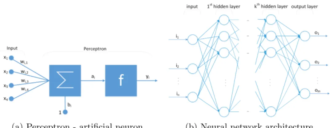
Fig. 2 shows the MLP architecture and a detailed view of the i-th

per-ceptron. A perceptron’s input is either the neural network’s input, if the perceptron is in the 1st layer, or the output of another perceptron in a previ-ous layer. Regardless of the origin, every incoming connection has a weight assigned to it, i.e., the strength of the signal. Input values are multiplied by the connection weight and combined by an aggregation function Σ. The

perceptron then applies an activation function f over the aggregated output

ai, which determines the output signal (yi).

(a) Perceptron - artificial neuron (b) Neural network architecture

Figure 2: Multi-Layer Perceptron Neural Network

The activation function is a non-linear function that determines how much a neuron is activated by its input, effectively mapping the aggregated input to the output. For example, if we needed our neuron to only return a value (activate) whenever the aggregated input value is above 5, we would do so with an activation function such as the one in Fig. 3. A sigmoid (Eq. 1) or a

(11)

Rectified Linear Unit (ReLU) (Eq. 2) are quite popular in recent literature, although we could also define our own.

Figure 3: Example activation function

sigmoid(x) = 1

1 +e−x (1)

ReLU(x) = max(0, x) (2)

(a) Sigmoid with different biases (b) Sigmoid with different weights

Figure 4: Sigmoid activation functions

Fig. 2 shows the bias term (bi) as input to the aggregation function. Its

purpose is to adjust the function along the input axis. Notice in Fig. 4a how the function is shifted by different biases, thus allowing us to set at which input value we want to centre the activation function.

Fig. 4b shows how the activation function is affected by different weights, for instance, we can see how a higher weight causes the sigmoid to go quicker from 0 to 1.

(12)

These weights are what a NN learns during training, which allows the NN to learn the distribution of the training data and use it to make predictions. With Fig. 2 in mind, let us see how the training process works:

1. Data: every data sample is made of an array of values, known as the features which characterise the sample, and a label. For example, in a health care dataset we may find as features the patient’s age, the sex and whether he does an annual check-up and the label could be the age at which he died.

2. Network initialization: weights are randomly initialized to a value be-tween 0 and 1; the bias term is initialized to 1.

3. Forward pass: the Input Layer receives the values of the first training samples and the perceptrons are applied layer by layer on the inputs and producing the outputs (from left to right).

4. Backwards pass: once the forward pass is complete, i.e., the last hidden layer has computed its output, the values of the Output Layer are compared to the values we expected and the error is measured; from the Output Layer we do a backwards pass (from right to left) updating the weights of every neuron depending on how responsible they were for the error (using the Back-propagation algorithm [2]).

5. Every forward and backwards pass over all the samples is called an epoch. The training process is an iteration of epochs.

The more epochs we test the network, the more it will learn, i.e., the closer the weights will bring the output of the network to the target output. However, by training for a large number of epochs we risk overfitting, which is when the network stops learning the data structure and starts learning the data instead [3], which in its turn will make the network less able to generalize and make good predictions with new data.

In addition to the specific perceptron parameters shown in Fig.2, the training process also depends on the following hyper-parameters:

• loss function: the function the network should use to evaluate the error of the prediction with respect to the target.

• optimizer: which strategy the network should follow to modify the weights, i.e., learn, in order to minimize the loss. A common strategy is to allow for significant changes in weights at the beginning of training and reduce their magnitude, as it progresses, for fine-tuning.

(13)

• batch size: samples are processed by the NN in groups and after every batch has been processed the weights are updated. Smaller batches require less memory to process and result in more frequent updates, hence the network learns faster and we can reduce the number of e-pochs. The downside is in the additional processing time and in the optimization process: NNs work by trying to minimize the loss, i.e., the difference between the predicted value and the target, if the weights are updated frequently and based on a small number of samples, the loss is going to fluctuate more than if we use a larger batch. As a result,

the loss between epoch i and epochi+ 1 can vary considerably.

2.2 Convolutional Neural Networks

CNNs are a type of NN which try to imitate how the brain processes images. In a series of experiments [4], [5], [6] the neurophysiologists David Hubel and Torsten Wiesel tried to determine the most basic facts about how the mammalian vision system works. Their findings were based on recording the activity of individual neurons in cats and monkeys’ brains and observing how they responded to images projected in precise locations on a screen in front of the animals. They discovered that neurons in the early visual system responded most strongly to very specific patterns of light, such as precisely oriented bars, but responded hardly at all to other patterns [7].

These studies inspired the neocognitron [8], which gradually evolved into

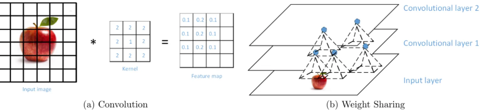
what are known today as CNN. An important milestone was the introduction of the LeNet-5 architecture [9], which built on previous efforts to create a system capable of recognizing handwritten check numbers. In this paper, the authors used fully connected layers (like the ones we saw in MLP) and sigmoid activation functions together with convolutional and pooling layers. As the name suggests, the basic operation of the convolutional layer is the convolution. A convolution applies a filter (or kernel) over the pixels of an image looking for specific patterns; the result is known as a feature map (Fig. 5a), which can be processed by higher layers in the CNN.

Fig. 5b conveys the idea of how every neuron is processing a small region of the image, pixels that are close together share the same weights. This idea makes CNN significantly more efficient than if we tried to have every pixel in the image linked to every neuron in the first hidden layer. It should be noted that by using weight sharing the network is able to leverage the pixels location information in its analysis.

Things to keep in mind when working with convolutional layers are the

stride, i.e., how many pixels do we move the kernel between convolutions, and the kernel size, bigger kernels can recognize more intricate features although

(14)

(a) Convolution (b) Weight Sharing

Figure 5: Convolutional Neural Network

they require more computation.

Pooling layers parameters are somewhat similar to convolutional, we need

to define the kernel size and the stride, although they do not have weights.

They are used to subsample the input image by aggregating pixels within the kernel region with an aggregation function, e.g,. mean, average, maximum. This allows for a reduced computational load, memory usage and limits the number of parameters in higher layers, hence limiting the risk of overfitting. Pooling the input also allows for some degree of location invariance, since the averaged result will be similar between shifted images even if the location is not exactly the same.

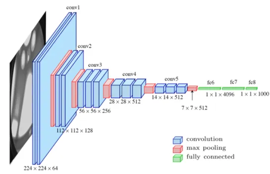
VGG-16 [10] is an example of a well-known CNN architecture. Fig. 6 shows how the different convolutional, pooling and fully connected layers are stacked to perform object recognition. We will work with VGG-16 when we look into image embeddings in the next sections.

2.3 Support Vector Machines

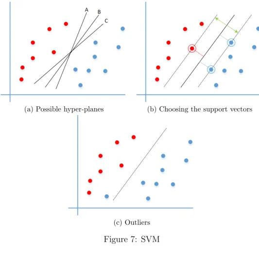
SVM is a supervised machine learning technique which can be used to solve classification as well as regression problems. It works by finding the best splitting boundary between the data points belonging to different categories, also known as the dividing hyper-plane.

Fig. 7a shows a few of the different hyper-plane options available to sep-arate data points belonging to two different categories. We mentioned above

that an SVM’s goal is to find the best splitting boundary; we now define

the best as the one with the widest margin to the closest data points with different labels, also known as the Support Vectors. In Fig. 7b we can see the Support Vectors from every group (circled), their distance to the hyper-plane and the hyper-plane’s margin in green.

(15)

Figure 6: VGG-16 architecture

Support Vectors, the rest of the training data will be ignored whenever we try to classify new data samples, which makes its execution quite fast.

Unfortunately, we will not always be able to neatly separate the data: sometimes the data is just not separable, other times outliers are the ones making the task difficult. For example, in Fig. 7c notice the blue sample on the red region. Normally, we have two options to deal with outliers:

• We can keep the original hyper-plane and control how flexible the SVM

algorithm can be, allowing some points to cross the boundary (effec-tively ignoring them). This may be a good option if we have a large number of samples and we are relatively certain that those points are really outliers.

• Otherwise, the SVM can look for a new hyper-plane that correctly

classifies all samples. The downside to this approach is that the new hyper-plane will have a narrower margin, which may result in poorer predictions for new data.

The balance between correctly classifying all the training samples and

obtaining the maximum margin possible is controlled with the C parameter:

(16)

a highCwill enforce correct classification with a narrower margin. We should fine tune this parameter on a per problem basis.

(a) Possible hyper-planes (b) Choosing the support vectors

(c) Outliers

Figure 7: SVM

Linear SVMs are good at working with linearly separable data, although that may not always be the case, see for example Fig. 8a. In those cases, we can use a function to map the original space into another one with a higher number of dimensions, where the data may be separable (Fig. 8b). This is

commonly referred to as the kernel trick, and depending on the function we

apply we will be working with a different SVM. The most commonly used functions, or kernels, are: polynomial, Radial Basis Function (RBF) and sigmoid. In Section 3, we will use an RBF to separate images.

2.4 Image Embeddings

As we saw earlier, CNNs try to imitate the way the brain processes images. During training, neurons focus on certain parts of an image and learn features which help them classify it. Classification is achieved when the neurons tied

(17)

(a) Non-linearly separable data (b) Kernel transformation

Figure 8: Kernel SVM

to features that belong to a particular class activate more than those tied to features that do not belong. Following this premise, a picture of a horse and a car should activate different sets of neurons.

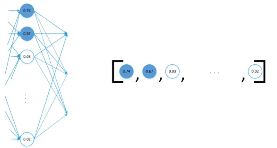
Figure 9: Embeddings: neuron activation used as a feature vector In a typical CNN performing a classification task, the last layer will usu-ally be a Softmax which will return the predicted label and its probability. For embeddings, however, we should focus on the layer immediately before,

a fully connected layer made of N different activations which, to reiterate,

represent features belonging to a class. Now, let us take this one step further and instead of thinking about a NN layer, imagine we rotate this layer on its side, see Fig. 9, and consider its output as a point in an N-dimensional space. This point is known as an embedding, the representation of the input image in that space. Theory suggests that points belonging to the same class should be closer to each other than to others, which allows us to use an SVM (or any other linear classifier) for image classification.

(18)

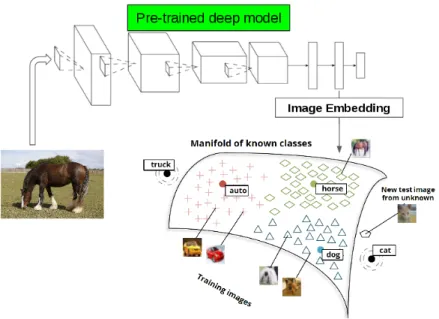
Figure 10: Image embedding space encoding its visual representation lan-guage

• During training, the N-dimensional space is partitioned in subspaces,

each belonging to a different class.

• Afterwards, if we consider images whose class was not used during

training, e.g., truck or cat, we can see that they fall relatively close to their most similar trained class (auto, dog).

Given a large training set, e.g., ImageNet 2012 [12] with 1000 classes, and a powerful deep learning model, e.g., the VGG-16 architecture [13] which includes 13 convolutional and 3 fully-connected layers, the resulting trained model should contain a large and rich visual representation language, i.e., features. These features could be used for other problems beyond the original purpose by training and applying a non-deep learning classifier, e.g., an SVM, on the embedding representation.

The process of applying knowledge learnt from one task to another is known as transfer learning. As a matter of fact, this case is defined as feature representation transfer by Pans et al. [14], or simply transfer learning for feature extraction.

One of the first works exploring the extraction and reuse of deep network activations was DeCAF [11]. In that work, the AlexNet [15] architecture, with 5 convolutional and 3 fully connected layers, is trained for the Ima-geNet 2012 challenge. After training, the authors freeze the weights on the network (ImageNet) and feed-forward images from new datasets, extracting

(19)

activations from the previous to last layer. As we noted before, these activa-tions are an embedding representation that encodes image information based on the visual language learnt by the model. One of the target datasets used is the SUN-397 [16] dataset, which contains scene images classified into:

• Outdoor man-made

• Outdoor natural

• Outdoor both

• Indoor

• Indoor and outdoor man-made

Fig. 11 [11] allows us to visualize those samples in the embedding space. Using this new representation, the authors evaluated different classification schemes using linear classifiers (SVM and/or Logistic Regression) and were able to outperform previous state-of-the-art classification approaches based on traditional hand-crafted features.

Figure 11: Images from the SUN-397 dataset colored based on their class. Their position corresponds to the learnt embedding space

2.5 Face detection

In this paper, we will leverage the work of [17] to detect faces in the image of every scene, which, according to the authors, outperforms other state of the art methods. Their paper proposes a cascaded CNN approach to predict face and landmark locations in an image. Fig. 12 [17] shows their pipeline:

1. They start by resizing the image being analyzed to different scales, thus building an image pyramid, which will be the input to the CNN.

(20)

Figure 12: Face recognition pipeline

2. In the first stage, a shallow CNN (Proposal Network, or P-Net, with 2 convolutional layers) produces candidate windows to contain a face. They use Non-Maximum Suppression (NMS) to merge highly over-lapped candidates.

3. After merging, the remaining candidates are fed to a second CNN called Refine Network, or R-Net, with 2 convolutional layers, which rejects a large number of false candidates and refines the bounding box around the face.

4. Last, a final CNN (3 convolutional layers) further refines the result and outputs facial landmark positions together with the level of confidence that the analyzed image is in fact a face.

It is worth noting that by cascading relatively shallow networks they are able to obtain good results (the edge of the precision-recall curve is at

[0.851,0.851], well above the other solutions against which their compare)

with relatively good computing performance.

In [18] we can find the Python implementation of cascading networks we will use in our solution.

2.6 Audio processing

It is quite common to apply computer vision models to audio processing with very few modifications, if any at all. One technique which makes this possible

(21)

is spectrogram analysis.

A spectrogram is a representation of how the frequency content of a signal changes with time [19]. Time is displayed along the x-axis, frequency along the y-axis, and the amount of energy in the signal at any given time and frequency is displayed as a level of grey or colour (see Fig. 13d). During regions of silence, and at frequency regions where there is little energy, the spectrogram appears white whereas dark regions indicate areas of higher energy.

[20] gives a very good introduction on spectrograms and how they are created. First, data digitally sampled in the time domain is broken up into segments. Then, the Fast Fourier Transform (FFT) is used to calculate the magnitude of the frequency spectrum for each part (Fig. 13a), also known as the spectrum. Next, that magnitude of frequency is transformed into a one column colour map (Fig. 13b). Finally, we repeat the process for every segment (Fig. 13c) and lay the results side by side to form the spectrogram image (Fig. 13d).

(a) From audio signal to frequency ampli-tude

(b) Transform frequency amplitude into a colour map

(c) Repeat and stack (d) Final spectrogram

(22)

Since the spectrogram is an image, we can use a CNN to try to learn patterns, like trying to identify specific sounds or phonemes if we are working with speech. However, research has shown that there are other techniques, e.g., Cepstral analysis or the Mel spectrogram, that can yield better results [20].

If we look at the spectrum in Fig. 14a, we will clearly see some peaks, marked with arrows, and some valleys. When working with a speech signal, those peaks denote the dominant frequency components. They are referred

to as formants and they carry the identity of the sound. Cepstral analysis

focuses on how we can separate the spectrum into individual formants, also

known as the spectral envelope, and the spectral details so that only the

important features of the envelope are analyzed.

As far as Mel-Frequency analysis is concerned, it is based on experimental evidence showing that the human ear acts as a filter and concentrates on certain frequency components. This is shown in Fig. 14b, which has more filters in the low frequency regions and less in high frequencies. Interestingly, the Mel-scale allows us to represent those signals so that sounds that feel similar to the human ear are close in the scale and apart otherwise. This is used to derive the Mel-Frequency Cepstral Coefficientss (MFCCs) in the following process:

1. Apply the FFT over the audio signal to obtain the spectrum.

2. Apply filters to obtain the spectrum, also known as the Mel-scale.

3. Take the logs of the powers at each of the Mel frequencies.

4. Take the discrete cosine transform of the list of Mel log powers, as if it were a signal.

5. The MFCCs are the amplitudes of the resulting spectrum.

In [21], the authors use various CNN architectures to classify the sound-tracks of a dataset of 70 million training videos (5.24 million hours), each tagged from a set of approximately 30000 labels. They examine and compare fully connected Deep Neural Networkss (DNNs), AlexNet [15], VGG [13], In-ception [22] and ResNet [23]. Their strategy was to:

1. Divide the audio into non-overlapping 960ms frames.

2. Each frame is decomposed into separate frequencies with a Short-Time Fourier Transform (STFT) applying 25ms windows every 10ms, thus overlapping the windows.

(23)

(a) Cepstral analysis

(b) Mel filters

Figure 14: Cepstral and Mel analysis

3. The spectrum is processed to build the Mel spectrogram.

For every architecture they analyze, the authors try to fine tune the networks by searching for the best hyper-parameters, e.g., for the DNNs they generate different combinations of the number of layers and the number of neurons in every layer, using between 10 and 40 GPUs.

As far as metrics are concerned they use the Area Under the Curve (AUC): probability of correctly classifying a positive example (correct accept rate) as a function of the probability of incorrectly classifying a negative example as positive (false accept rate); perfect classification achieves AUC of 1.0.

Their results show that while fully connected DNNs achieve an AUC of 0.851, they are outperformed by all other computer vision architectures, being ResNet-50 the superior model.

[24] trains a CNN on the TIMIT [25] dataset for speaker recognition. TIMIT contains studio quality recordings of 630 speakers (192 female, 438 male), each reading 10 phonetically rich sentences, sampled at 16KHz, cov-ering the eight major dialects of American English. They first compute the Mel-spectrogram with 128 elements in frequency direction for each sentence of the dataset, preserving the 16KHz original sampling rate, taking 1024 sam-ples FFT window length and 160 samsam-ples as hop length. They then perform dynamic range compression of the spectrograms by applying the element-wise

function f(x) = log(1 +C ∗x) with C = 10000. Finally, they extract one

second long snippets of non-overlapping pieces from the spectrograms and use these images of 128 x 100 pixels as the basic input to the CNN (Fig. 15 [24]).

(24)

With this setup, the authors report a 97% accuracy, thus correctly iden-tifying 611 out of the 630 speakers.

Figure 15: CNN architecture

[26] proposes using very deep CNN that directly use time-domain wave-forms as inputs. The major disadvantage of this approach is the amount of processing power it requires. The authors try to mitigate this by down-sampling the audio from 16KHz to 8KHz, and by customizing the receptive field of the first convolutional layer to only cover 10-millisecond duration, thus looking to reduce the number of weights by taking advantage of the weight sharing feature in the convolutions.

They tested different architectures with 3, 5, 11, 18 and 34 convolutional layers over a dataset consisting of 8732 audio clips of at most 4 seconds, totalling 9.7 hours. The performance was measured in absolute accuracy and they obtained the best results for the architecture of 18 layers (71.68%).

In [27], the authors work with Convolutional Deep Belief Networks (CDBNs) to classify audio, learning features in an unsupervised manner and outper-forming spectrograms and MFCCs. CDBNs are based on Convolutional Re-stricted Boltzmann Machines (CRBMs), which in their turn are an extension of the regular Restricted Boltzmann Machine (RBM) to a convolutional set-ting.

(25)

RBMs [28], [29] are a two-layer network where stochastic binary pixel-s are connected to pixel-stochapixel-stic binary feature detectorpixel-s upixel-sing pixel-symmetrically weighted connections (Fig. 16). The pixels correspond to ‘visible’ units of the RBM because their states are observed; the feature detectors correspond

to ‘hidden’ units. A joint configuration of the visible and hidden units (v, h)

has an energy given by:

E(v, h) =− X i∈visible aivi− X j∈hidden bjvj − X i,j vihjwij (3)

wherevi, hi are the binary states of visible unitiand hidden unitj,ai, bj

are their biases and wij is the weight between them.

The network assigns an energy to every (v, h) configuration. While being

trained, the weights are adjusted so that the energy assigned to the training configurations is low, i.e., the RBM effectively learns a pattern so that dur-ing testdur-ing, the samples resembldur-ing the traindur-ing configurations will have low energy as well.

RBMs can be used for multi-category classification if we add the label to the input data and when testing, for every sample we add all the possible categories it can predict; the right category will be the one with the lowest energy.

CRBM is an extension of the regular RBM to a convolutional setting, in which the weights between the hidden units and the visible units are shared among all locations in the hidden layer. The authors stack multiple CRBMs to obtain a CDBNs.

For the application of CDBNs to audio data, the authors first convert time-domain signals into spectrograms and reduce their dimensionality by applying PCA-whitening, going from 160 components to 80. Spectrograms were created with a 20ms window size and a 10ms overlap.

Table 1 [27] show the results, measured as accuracy, of speaker identi-fications comparing CDBNs vs. MFCC features [30] vs. combining both approaches. We can see that in all cases CDBNs perform equally or better than MFCC, and in all cases the combination of features outperforms them by separate.

The authors follow a similar approach to do gender classification and phone classification with similar results.

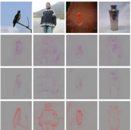
[31] discusses Layer-wise Relevance Propagation (LRP), a technique ap-plied to image processing which assigns a relevance score to every pixel of an image depending on how much it contributes to its correct classification. In a nutshell, their idea is to start at the output layer assigning a relevance score to every neuron and work their way back layer by layer until reaching the input. Fig. 17 shows how with different hyper-parameters LRP successfully

(26)

#training utterances per speaker MFCC [30] CDBN MFCC [30] + CDBN 1 40.2% 90.0% 90.7% 2 87.9% 97.9% 98.7% 3 95.9% 98.7% 99.2% 5 99.2% 99.2% 99.6% 8 99.7% 99.7% 100.0%

Table 1: Speaker identification accuracy with CDBNs

shows on which parts of the image the neural network focuses to perform classification.

Figure 17: Original images (top row) and Layer-wise Relevance Propagation applied with different parameters

In [32] the authors build on the work of [31] (LRP) applying it to the classification of audio signals. They build their own dataset, AudioMNIST [33], which consists of 30000 audio recordings (approximately 9.5 hours) of spoken digits (0-9) in English with 50 recordings per digit from each of the 60 different speakers. They annotated the dataset to include the speaker’s age, gender, origin and accent.

Using this data they built two classifiers, one working with spectrograms and another with raw waveforms.

• Spectrograms: audio recordings were re-sampled to 8KHz, zero-padded

to a fixed signal dimensionality of 8000 and transformed to a spectro-gram representation via STFT. STFT parameters were set to yield spectrograms of dimensions 228 x 230 which they cropped to 227 x 227

(27)

by discarding the highest frequency bin and the last two time-bins. The amplitude was converted to decibels and used as input to the network. They used a modified version of AlexNet [15].

• Raw waveforms: processed by a CNN, which the authors call AudioNet,

inspired by the one described in [10]. As with spectrograms, audio recordings were re-sampled to 8KHz, zero-padded to a fixed signal di-mensionality of 8000. They added two dummy axes to represent width and depth, required by the convolution operation of the CNN’s first layer. Finally, the signal was normalized by the waveform’s 95th am-plitude percentile. They did not use the maximal amam-plitude due to outliers which they attribute to environmental noise.

The authors applied these classifiers to solving digit and gender recog-nition. Table 2 [32] shows how, consistent with what we have seen so far, spectrogram analysis yields better results than waveform.

Architecture Input Digits Gender

AlexNet Spectrogram 95.82% 95.87%

AudioNet Waveform 92.53% 91.74%

Table 2: Accuracy: spectrogram vs. waveform

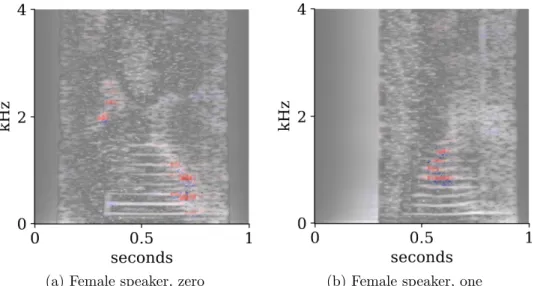
Fig. 18 shows the LRP analysis of a spectrogram. For digit classification, the authors do not know how these pixels in the image map to higher con-cepts, such as phonemes, although they hypothesize that gender classification is based on the fundamental frequency and its immediate harmonics.

Fig. 19 shows the LRP analysis of a raw waveform used for gender classifi-cation. Fig. 19c is particularly interesting as it shows that the network focuses on the signal points with a greater magnitude. We believe it would be inter-esting to perform an experiment where the raw waveform is pre-processed in a way that removes all the intermediate points, verify the impact on network accuracy and see how much computing power it saves.

VoxCeleb [34] uses spectrograms for speaker identification and verifica-tion. They first start by creating their own dataset by setting an automatic pipeline:

• Obtain a list of people: they use the VGG Face dataset [35] as a list of

celebrities names (2622 identities).

• Download videos from YouTube: the top 50 videos for every name are

(28)

(a) Female speaker, zero (b) Female speaker, one

Figure 18: Spectrograms as input to AlexNet with relevance maps overlaid

(a) Male speaker, zero

(b) Heatmap: positive relevance in favour of class male is coloured in red and negative relevance, i.e., relevance in favour of class female is coloured in blue

(c) Selected range of the waveform above where single samples are coloured according to their relevance

Figure 19: Gender classification of the raw waveform of a spoken zero

• Face tracking: they use the HOG-based face detector [36] to detect

faces in every frame of the video.

• Active speaker verification: verifies that the person in the video is

(29)

• Face verification: they use VGG-16 trained on the VGG Face dataset to identify the faces. The authors substitute manual annotation by setting a high threshold, i.e., if the network identifies a face with a confidence below the threshold the sample is rejected and not included in the dataset.

The result of this process is the VoxCeleb dataset, which contains auto-matically tagged utterances from over 1000 celebrities. The authors use the dataset to conduct speaker identification experiments.

The audio is first converted to single-channel 16-bit streams at a 16KHz sampling rate for consistency. They generate spectrograms in a sliding win-dows fashion using a hamming window of 25ms of width, 10ms step and 1024-point FFT. This returns spectrograms of size 512 x 300 for 3 seconds of speech. They perform mean and variance normalization on every frequency bin of the spectrum, which according to the authors leads to an almost 10% increase in classification accuracy. These short time magnitude spectrograms are used as input to a CNN.

The paper uses a variation of the VGG-M [37], replacing some layers to make them invariant to temporal position but not frequency.

They report results of a 80.5% classification accuracy for speaker identi-fication, 20% higher than state of the art solutions.

(30)

3 Speaker identification

3.1 Introduction

Leaving the background and state-of-the-art behind, we will now focus on building our dataset and creating new models for image-based speaker recog-nition, audio-based and a combined model. We will explore different tech-niques and set-ups in the search for increased accuracy.

The first step is to build a tagged dataset of both images and audio fragments categorized by person. After careful consideration, we chose the Parks and Recreation (PR) TV series as our data source because of the way it was filmed: PR is a mockumentary following the life of city-hall employees, most of which occurs in a well-lit building. For the record, it also features outdoors scenes, at night and with background music, although in a lesser amount.

We purchased the DVD set for the entire series and used ffmpeg [38] to extract the audio and the images we required. The sections below give more information on the process we followed to convert every episode into short scenes and from those scenes how did we collect the characters’ faces. Final-ly, we matched the samples with their belonging character, thus manually classifying more than 4000 pictures and 11000 audio samples.

After building the dataset we will start experimenting with image recog-nition:

• We will begin by building a CNN architecture which is able to

distin-guish between any of the 10 members of the PR cast.

• Data augmentation will be applied to the dataset to see if (i) there are

any performance gains and (ii) it could be used to reduce the size of the dataset while maintaining accuracy (and therefore reduce the effort required to manually classify the samples).

• Using the best model trained with data augmentation, we will freeze the

weights and analyze its predictions when processing images containing faces from other people or even no faces at all. We expect to see low predicted probabilities in all the 10 characters. This should allow us to reject unknown samples by establishing a probability threshold so that all samples with a smaller predicted probability can be discarded without affecting the model’s performance.

• We will use transfer learning to obtain image embeddings and classify

them with an SVM. Its performance will be compared against the CNN model.

(31)

Next we will focus on processing the audio, mirroring the experiments we defined for images:

• We will define how to create the spectrograms from every segment.

• Build a spectrogram-based CNN for character identification.

• Determine the impact of spectrogram length in the model’s accuracy.

• Propose a data augmentation technique for spectrograms and measure

its validity.

• Observe how does the best trained model behave when processing

sam-ples from music and unknown voices.

Finally, using Keras [39] functional API, we will define a multi-input network which processes faces and spectrograms at the same time. Different architectures will be applied and compared against each other.

It should be noted that for every experiment, data will be divided into training (68%), validation (12%) and test (20%) sets. Data augmentation, when applied, will only be performed over the training set.

3.2 Image based identification

3.2.1 Data pre-processing

Our first approach to split every video episode into scenes or

sentences/utter-ances was to use pauses (silences) in the audio. We tried usingauditok [40], a

software tool for audio tokenization which is supposed to be able to recognize audio activities based on a signal threshold set by the user. We tried fine tuning the threshold over different scenes but the results were unsatisfactory, with segments cut mid-sentence.

Instead, we went in another direction and used the subtitles, which in addition to the audio transcription, contains the time start and end of every utterance. With this information we split each episode into short scenes from which we extracted the audio (sampling at 16KHz) and the first image.

The next step was to focus on how to obtain the faces from every scene. As detailed in Section 2.5, we used MTCNN [17] for face detection. Its imple-mentation by [18] worked out of the box and even though we experimented with its hyper-parameters we obtained the best performance with the de-faults. Fig. 20 [18] shows how the algorithm returns a bounding box around a face and the location of a set of features (eyes, nose and mouth).

(32)

Figure 20: MTCNN face detection - boxing and features

We processed the scene images through the algorithm and created a dataset just containing the characters faces. The face images were also re-sized, since a CNN requires all input samples to be of the same dimensions. These were manually labelled and became the dataset for the next phase, with 400 face pictures per character.

3.2.2 Face recognition - part 1: CNN

Once we had compiled a face dataset, we were able to start experimenting with a CNN for face recognition. Fig. 21 shows the architecture we put together by stacking convolutional, pooling and fully connected layers. The dropout layers were added after our firsts experiments and are responsible for an approximate 5% increase in accuracy (see Section A.2 for more information on the layers parameters). Functionally, dropout consists in randomly setting a fraction of input units to 0 at each update during training time, which helps prevent overfitting. Theory suggests they may increase the model’s overall performance by making the layers on top (further away from the input) more resilient to the loss of information.

The model was trained for 2437 epochs over 272 images for each catego-ry (2720 total), we used early stopping with a patience of 500 epochs and checkpointing the weights with the best validation accuracy. Fig. 22 shows the accuracy and loss over the training process, how the model is able to reach nearly 1.0 accuracy and almost 0 loss on the training data yet it ends up stagnating with the validation set. This model yielded an accuracy of 0.936 and loss of 0.288 over the test data.

Looking into ways to improve the model’s performance without having to

invest more time in manually tagging new images we found the

ImageData-Generator provided by Keras [39]. Basically, instead of feeding the training data to the model we fed it to the generator which randomly altered the images before passing them on to the model. The code excerpt below shows the used transformations:

(33)

Figure 21: CNN architecture

(a) Accuracy by epochs (b) Loss by epochs

Figure 22: CNN trained for face recognition

# random r o t a t i o n ( d e g r e e s , 0 t o 1 8 0 ) r o t a t i o n r a n g e =10 , # r a n d o m l y s h i f t i m a g e s h o r i z o n t a l l y ( f r a c t i o n o f t o t a l w i d t h ) w i d t h s h i f t r a n g e = 0 . 1 , # r a n d o m l y s h i f t i m a g e s v e r t i c a l l y ( f r a c t i o n o f t o t a l h e i g h t ) h e i g h t s h i f t r a n g e = 0 . 1 , # s e t r a n g e f o r random zoom z o o m r a n g e = 0 . 3 , # s e t mode f o r f i l l i n g p o i n t s o u t s i d e t h e i n p u t b o u n d a r i e s f i l l m o d e= ’ n e a r e s t ’ , # r a n d o m l y f l i p i m a g e s h o r i z o n t a l f l i p =True )

Listing 1: Data augmentation configuration

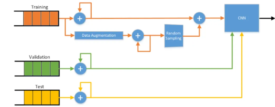
It should be noted that data augmentation was only applied to the train-ing set, not to validation nor test. Fig. 23 depicts the pipeline.

(34)

Figure 23: CNN experiment pipeline

epochs and yielded a test accuracy of 0.956 and test loss of 0.159, thus outperforming the previous result by a 2% margin. Fig. 24 shows the training process. It should be noted how the validation accuracy and loss now seems to almost overlap with the results for the training data.

Starting with 2720 training pictures, through data augmentation the net-work ended up using almost 7 million.

Comparing this with the basic CNN, we can see this one trained for almost 500 more epochs. One may wonder if the difference between one experiment and the other comes from the extra training epochs instead of from using data augmentation (despite having the same patience). Therefore, we repeated this experiment with augmented data and fixed the maximum epochs to 2061. This yielded a 0.954 accuracy and 0.1967 loss, still outperforming the original results and showing that data augmentation does improve the model.

(a) Accuracy by epochs (b) Loss by epochs

Figure 24: Best CNN with data augmentation

Looking at those results we wondered how much we could decrease the number of labelled images, while still using data augmentation to compensate

(35)

the difference, without affecting the model’s performance. For consistency

(and repeatability), we used theImageDataGenerator to generate augmented

images over the training dataset beforehand and split them into 30 batches of 1000. The model was modified to test over every batch iteratively:

1. Train over every batch (patience= 500).

2. When it stops, measure performance with test set.

3. Use the checkpointed model, i.e., the one with the best validation ac-curacy during training, and test it with a new batch of augmented images.

Fig. 25 shows the comparison between using 68 images per character, 136, 204 and 272. The first thing we see is the 68 images accuracy and loss fall behind the other three options. Looking at it with more detail we observe that 136 is always below 204 and 272 and that 204 and 272 intersect at multiple locations, thus indicating that neither options is significantly better than the other. This allows us to conclude that using data augmentation, we could decrease our training dataset size to 204 images per character without impacting performance.

Finally, we should note that even with 30000 augmented samples, the best accuracy was around 0.93, thus showing that using pre-partitioned sets

of augmented images is not the best option (as opposed to an online

Image-DataGenerator).

(a) Accuracy by samples (b) Loss by samples

(36)

3.2.3 Facing something unknown

Even though the MTCNN [18] does a good job identifying faces in video frames, it is not perfect and there are times where our character recognition CNN is going to receive non-face images. In addition, we need to be able to discriminate between the main characters and random extras appearing in a given scene. To that end we manually tagged a smaller fraction of images not showing a face or showing other characters (extras) faces.

In this experiment, we froze the weights of the best CNN with data aug-mentation and ran it over the training, validation, other characters and non-faces image data sets and observed the probabilities of the Softmax in the last layer. What we expected to see is that the probabilities for the trained characters would be high and probabilities for extras and non-faces would be low, thus allowing us to set a probability threshold that would allow us to discard unwanted images.

Fig. 26 shows the results of the experiment. For each probability threshold we plot how many samples (proportion) are above it. If we look at the faces validation data, we can see that over 80% of the samples are correctly

classified with a predicted probability≥0.90, i.e., that 20% of the samples are

predicted with a probability<0.90. If we look at faces from other characters

or non-faces, we can see that approximately 10% are identified as one of the

main characters with a probability ≥ 0.90. This means that if we set the

threshold to 0.90 the accuracy of the network will be negatively affected by both misclassifying some of the main characters as well as other characters and non-faces.

Figure 26: CNN predicted probabilities: trained faces (Training) vs. new images of trained faces (Validation) vs. images of other faces (Others) vs. images of not faces (Non-faces)

To try to improve on these results, we decided to implement a one vs.

(37)

C’s samples as positive samples and all the other’s as negative. We applied data augmentation and early stopping with patience of 500 epochs. The first thing we noticed is that the accuracy over the test dataset was higher than the best CNN with data augmentation from section 3.2.2, which could be explained by the fact that recognizing a character is easier than recognizing

10. Fig. 27 shows the accuracies for classifying all the test samples per

character: average accuracy is 0.987, with a minimum accuracy of 0.976 for one of the characters.

It should be noted that we did not change the architecture, hence we used 10 CNNs trying to solve the same problem (divide and conquer approach). We also expected some difficulties during training as there are 9 times more negative samples than positive; however, that was not the case.

Figure 27: 1 against all CNN: classification accuracy

Once again, we froze the weights and tried to classify faces from other actors (others) and non-faces (Fig. 28). Other faces yields an average accu-racy of 0.95 and non-faces a 0.935. Note how some characters are worse than others, which means they are more easily confused with other people (Jerry, Leslie) or things (Jerry, Leslie, Dona).

Finally, we combined the 10 different models into one by adding a layer at bottom which processes the predicted probability of every individual model and outputs a label for one of the main characters. We froze the layers of the individual models and trained the new layer with the training data. This new model yields an accuracy of 0.95, similar to the results obtained by the CNN with data augmentation presented in the previous section (0.956). Although, it is interesting to note this is much more consistent in prediction, always on 0.95x whereas the other model went from 0.94 to 0.96.

Fig. 29 shows how training is significantly faster, which is to be expected since the individual model layers are frozen and we are only training the new layer at the bottom.

(38)

(a) Other faces (b) Non-faces

Figure 28: One vs. all CNN: other faces and non-faces

(a) Accuracy (b) Loss

Figure 29: 10 One vs. all CNN assembled together

As far as predicted probabilities go, Fig. 30 shows how the samples are distributed. The first thing to notice is that the highest probabilities in the network are below 0.40; there are no samples above it. The minimum probability in the validation dataset is of 0.20, whereas the maximum of other faces is 0.42 and 0.39 for non-faces. Once again, there does not seem to be a clear probability boundary that indicates an image does not belong to the main cast.

We leave as future work further experimentation with this ensemble ar-chitecture (adding more layers) and looking into Siamese Networks [41], a particular kind of networks which are trained by recognizing images that look similar but that are different, and as a result are more resilient to un-known samples.

(39)

Figure 30: Ensemble CNN predicted probabilities: trained faces (Training) vs. new images of trained faces (Validation) vs. images of other faces (Oth-ers) vs. images of not faces (Non-faces)

3.2.4 Face recognition - part 2: image embeddings

In this section we decided to experiment with image embeddings, as defined in Section 2.4. Fig. 31 shows the proposed pipeline:

1. Use data augmentation for the training dataset.

2. Feed the training, validation and test data to a VGG-16 architecture pre-trained with the ImageNet dataset (weights frozen).

3. Obtain the activation of the last fully connected layer and use it as the image embedding.

4. Classify the embeddings with an SVM.

Fig. 32a shows the accuracy results for SVM without data-augmentation, 0.766, well below the 0.936 obtained with a CNN with the same data (2720 training samples).

Fig. 32b shows our attempt to run an SVM with data augmentation pro-ducing as many samples as our hardware would process (150000). Originally, we tried with 300000 but the SVM did not scale well as the dataset size grew. The results in the image show an accuracy slightly over 0.83, an improvement but still below the CNN results (0.956).

Finally, we tried to repeat the detailed study of how accuracy grows as we increase the use of augmented data. Interestingly enough, 204 and 272 samples yield similar results, as we saw in the CNN experiment (Fig. 25a).

(40)

Figure 31: Embedding experiment pipeline

(a) Original data (b) With data augmentation - overall best

(c) Data augmentation impact

(41)

3.3 Audio based identification

3.3.1 Data pre-processing

For this part of the project we needed to create a voice dataset using audio from the TV-show. We followed the same process described in 3.2.1 and took an audio sample from every utterance.

We examined and tagged over 11000 audio samples (Fig. 33a), and we noticed that (i) a large number of samples were invalid (multiple voices, noises, only music, etc.) and (ii) getting enough samples from the some of the actors would require a very long time with this process. Hence, we decided to pad some of the characters samples with their actors’ interviews on Youtube (Fig. 33b).

(a) TV-show (b) TV-show + Youtube

Figure 33: Audio sample distribution by character

Having built the dataset, we started investigating how we could extract the spectrograms. The authors of [34] generate spectrograms in a sliding window fashion using a hamming window of width 25ms, step 10ms and 1024-point FFT; we followed the same approach and defined as well the Mel scale with 128 bins, based on [24].

[34] processes audio in 3s segments. However, due to the nature of our dataset, if we were to follow the same approach, we would be discarding a significant portion of shorter audio samples. Hence, we decided to start with 1s spectrograms.

3.3.2 Audio CNN

The next step after creating the spectrograms was to define a CNN archi-tecture appropriate for voice recognition. [34] uses a modified version of the

(42)

VGG-M [42], which they test on a Nvidia Titan X GPU. Given our more lim-ited resources, we tried a similar architecture albeit with reduced dimensions (depicted in Fig. 34).

Figure 34: Audio CNN

Just like for image recognition, we will be using early stopping although with less patience, 100 epochs.

Fig. 35 shows the training process over accuracy and loss, notice how the model stops learning at around 0.6 accuracy. Using 588 samples per character, we were able to obtain an accuracy of 0.67 on the test dataset.

Figure 35: Voice recognition - all characters

Given the gap in samples between main and supporting characters, we decided to repeat the experiment just by looking at the top-4, i.e., the 4

(43)

characters with more samples. Fig. 36 shows accuracy and loss during train-ing, notice how the distance between the validation and training curve is now reduced by almost half. Using 962 samples per character, we obtained an accuracy of 0.824 on the test set, significantly improving the previous results. However, we should note that classifying samples from 4 classes is simpler than classifying from 10. We repeated the top-4 classification with a reduced dataset (588 samples) and obtained an accuracy of 0.72, thus showing that both problem simplification and a bigger dataset share credit for the overall improvement.

Figure 36: Voice recognition - top 4

We experimented with different combinations of hyper-parameters and architectures and these were the best results we obtained. It is interesting to note that the face recognition network we used in the previous section yielded a 0.784 accuracy on the top-4 dataset, without any modifications.

3.3.3 Data augmentation

Considering the difficulty of gathering samples for some of the characters, we once again looked for some form of data augmentation. We hypothesized that the network should be able to recognize a given sound (frequency) re-gardless of its position in the spectrogram. Hence, we created spectrograms in a sliding window fashion (Fig. 37), i.e, for every sample we (i) took a 1s segment, (ii) created the spectrogram, (iii) slided the window 100ms and repeated from (i).

We designed a experiment where we applied the technique described above to the training dataset; we were mindful not to have training, vali-dation and test share any sample-augmented sample pair. We ran the CNN over the data with at most [0, 1, 2, 3, 4, 5] augmented samples (cannot

(44)

guar-Figure 37: Sliding window sampling with overlap

antee the exact number of augmented samples we could generate from an audio slice since segments vary in length).

Fig 38 shows the results for the top-4 characters: we can see that as we increase the samples, the accuracy increases, with a best result of 0.904 with over 12000 samples. The improvement is greatest when going from 0 (2616 samples) to 3 (9922 samples), going from 0.824 to 0.889.

These results show that the data augmentation technique does help im-prove the model.

A similar improvement can be seen in the 10 classes experiment (Fig.39), going from an accuracy of 0.67 to 0.788 with 20974 samples.

3.3.4 Spectrogram length

In this experiment intend to verify if the length of the spectrogram has an impact on the model’s performance. To that end, we defined a new set of spectrograms of length 500ms (as opposed to the 1s used earlier) over the same audio data, which resulted in twice as many images.

Using 500ms spectrograms for the top 4 characters, the model yielded a 0.802 accuracy and 0.500 loss, vs. the 0.824 accuracy and 0.463 loss obtained by the 1s experiment in 3.3.3, hinting that longer spectrograms are better.

(45)

Figure 38: Voice recognition - Top 4

Figure 39: Voice recognition - All

This goes in line with the results shown by [34], where the authors select 3s spectrograms. It is worth pointing out that they were able to work with long audio segments because they processed interviews, where the conversational pattern is usually a short question and a long answer, as opposed to our dataset where the pattern is usually people talking naturally and interjecting each other.

3.3.5 Music and other voices

In this section we wanted to examine the predicted probabilities of a trained network when facing new data. To that end, we took the network trained over top-4 with at most 4 augmented samples per original (accuracy 0.90) and looked into its predicted probabilities when processing (i) new data of the voices on which it was trained (test set), (ii) new voices and (iii) music. The first thing we notice when looking at Fig. 40a is that 94.5% of the

(46)

samples which are correctly classified have a probability above 0.9. Fig. 40b shows that for new voices the proportion of samples above 0.9 is 36.1% and Fig. 40c shows 20.2% for music. This means that if we were to set a prob-ability threshold on 0.9, i.e., samples below 0.9 are considered invalid, we would be able to discard about 80% of the music samples and 74% of new voices, thus indicating that spectrogram recognition is more resilient than face recognition (Section 3.2.3), even if the character accuracy is lower.

(a) Predicted probabilities - test set (b) Predicted probabilities - other voices

(c) Predicted probabilities - music

Figure 40: Recognizing new sounds - predicted probabilities

3.4 Image & audio identification

In our last experiment with spectrograms and augmented data for all the characters we pushed the limits of our hardware set-up. The model itself required 11GB of memory (our graphics card has 11.1GB) in addition to a bigger swap partition, since the data went over the available memory. Hence, before looking into how to build the combined model itself we needed to find a way to improve our pipeline.

(47)

By default, LibROSA [43] generates colour spectrograms with differen-t colours indicadifferen-ting differendifferen-t energies. However, we hypodifferen-thesized differen-thadifferen-t we should be able to obtain the same results by using a grey scale, which would allow us to go from 3 channel images to 1.

We repeated the top-4 and the all classification experiments with da-ta augmenda-tation and obda-tained similar results, top-4 0.898 accuracy and all 0.798, thus confirming the hypothesis.

This allowed us to work with smaller samples (we used 1 channel instead of 3), which decreased the amount of RAM memory needed by 2/3 and freed up some space on the GPU to start working on the combined model.

Figure 41: Image & Audio CNN

Fig. 41 shows our proposed architecture. We decided to create a new network which takes two inputs: (i) a face image and a (ii) spectrogram image. To that end we took the Head of the Spectrogram CNN (all layers before and including flattening the features) and the Head of the Face Image CNN (Fig. 21), concatenated the resulting features and fed them to the Spectrogram Tail (the fully connected layers after the flattening) (see Section A.4 for the definition). Our reasoning for using the spectrogram tail was that it being the most powerful of the two it could work with both faces and

(48)

spectrogram features.

We tested the architecture by using 400 pairs of character’s faces and spectrograms (just like we did in Section 3.2.2). The results are depicted in Fig. 42: accuracy of 0.899 and loss of 0.312 vs. 0.936 and 0.288 of the original experiment where we used a CNN over face images (without data augmentation).

Figure 42: Combined results - without data augmentation

In order to compare the best joint model with the best overall model so far (CNN over faces with data augmentation - accuracy of 0.956) we needed to apply data augmentation as well. This posed a problem since we could not augment spectrograms in the same way we augment faces. Instead, we decided to use the augmented spectrograms we had (with up to 5 samples per original) and randomly match them with an original or an augmented face image of the same character.

This set-up yielded an accuracy of 0.901 and a loss of 0.357, Fig.43, thus showing that in this scenario data augmentation did not make an improve-ment.

It is interesting to note that from a spectrogram-only point of view (ac-curacy 0.788), the combined model is indeed an improvement. This result suggests that combining a good classifier with a mediocre one reduces per-formance since the joint model is unable to learn when to rely on one or the other.

We tried slight changes to the architecture with different results:

1. V2: back when we were designing the face recognition CNN, we recall that too many or too large layers after flattening the input resulted in lower performance. Hence, we tried simplifying the tail (see Section A.5), although this resulted in an accuracy of 0.712.

(49)

Figure 43: Joint results - with data augmentation

2. V3: we also tried changing the point at which we merged both networks (see Section A.6), instead of merging right after flattening we allowed the spectrogram head to include 2 convolutional layers from the tail. Accuracy 0.823.

3. V4: finally, we decided to let the networks run separately and join them before the Softmax with a fully connected layer (Section A.7 - Fig. 44). This gave a similar performance to v1 (0.889 accuracy).

(50)

We were surprised by these results. At the very least, we believe the joint model should perform at least as well as the face image CNN on its own. Logically, the network should learn not to rely on spectrograms if they do not contribute to the right prediction. Although that may require a larger dataset.

Following up on this intuition, we examined the learnt weights of the 4 versions of the model at the first fully connected layer after the concatenation. We computed the average weights connecting to the image CNN and the average for the spectrogram. Results are shown in Table 3.

Architecture Face weights Spectrogram weights Accuracy

v1 0.00077 0.00037 0.90

v2 0.00107 0.00052 0.712

v3 0.00024 0.00038 0.823

v4 0.00180 0.00263 0.0889

Table 3: Joint models average weights

These show that the joint model is drawing input from both networks. For instance, despite relying differently on faces and spectrograms, v1 and v4 perform similarly.

We hypothesize that the joint model requires more data to be able to learn as well as each model does by separate. To verify this hypothesis, we prepared one final experiment were we tried to reduce the number of trainable parameters:

1. We trained a face image CNN with data augmentation and stored the weights. We also persisted which images where used as train, test and validation.

2. We trained a spectrogram CNN with data augmentation (5 augmented samples) and stored the weights and the train/test/val data distribu-tion.

3. Using model v4 (Fig. 44 - Section A.7), which consists basically of the original networks with an additional fully connected layer connecting them, we initialized its layers to the individually trained weights and froze them. The only layer we were going to train is the fully connected we added at the end.

4. Merged train faces with train spectrograms, validation with validation and test with test.