Wavelet penalized likelihood estimation in generalized functional models

Wavelet penalized likelihood estimation in generalized

functional models

Ir`

ene Gannaz

To cite this version:

Ir`ene Gannaz. Wavelet penalized likelihood estimation in generalized functional models. test, Springer, 2013, 22 (1), pp.s11749-012-0310-6. <10.1007/s11749-012-0310-6>. < hal-00577733v2>

HAL Id: hal-00577733

https://hal.archives-ouvertes.fr/hal-00577733v2

Submitted on 19 Sep 2013

HAL is a multi-disciplinary open access archive for the deposit and dissemination of sci-entific research documents, whether they are pub-lished or not. The documents may come from teaching and research institutions in France or abroad, or from public or private research centers.

L’archive ouverte pluridisciplinaire HAL, est destin´ee au d´epˆot et `a la diffusion de documents scientifiques de niveau recherche, publi´es ou non, ´emanant des ´etablissements d’enseignement et de recherche fran¸cais ou ´etrangers, des laboratoires publics ou priv´es.

Wavelet penalized likelihood estimation in generalized functional

models

France.

[email protected]

Abstract

The paper deals with generalized functional regression. The aim is to estimate the influence of covariates on observations, drawn from an exponential distribution. The link considered has a semiparametric expression: if we are interested in a functional influence of some covariates, we authorize others to be modeled linearly. We thus consider a generalized partially linear regression model with unknown regression coefficients and an unknown nonparametric function. We present a maximum penalized likelihood procedure to estimate the components of the model introducing penalty based wavelet estimators. Asymptotic rates of the estimates of both the parametric and the nonparametric part of the model are given and quasi-minimax optimality is obtained under usual conditions in literature. We establish in particular that theℓ1

-penalty leads to an adaptive estimation with respect to the regularity of the estimated function. An algorithm based on backfitting and Fisher-scoring is also proposed for implementation. Simulations are used to illustrate the finite sample behaviour, including a comparison with kernel and splines based methods.

KEYWORDS: Generalized partially linear regression; semiparametric models; M-estimation;

penalized loglikelihood estimation; wavelet thresholding

1

Introduction

The aim of this paper is to consider a regression model, where the responseY is to be predicted by covariates z, with Y real-valued and with z a real explanatory vector. Relaxing the usual assumption of normality, we consider a generalized framework. The response value y is drawn from a one-parameter exponential family of distributions, with a probabilistic density of the form:

exp yη(z)−b(η(z)) φ +c(y,φ) . (1)

In this expression, b(·) and c(·) are known functions, which determine the specific form of the distribution. The parameter φ is a dispersion parameter and is also supposed to be known in what follows. The unknown function η(·) is the natural parameter of the exponential family, which carries information from the explanatory variables. Given a random sample of sizendrawn independently from a generalized regression model, the aim is to predict the functionη(·). Such a model gives a large scope of applications because observations can result from many distribution families such as Gaussian, Poisson, Binomial, Gamma, etc. For a more thorough description of generalized regression modeling, we refer to McCullagh and Nelder(1989) orFahrmeir and Tutz (1994).

In the following z = (X,t), with X a p-dimensional vector and t a real-valued covariate. The functionη(_·)is given by:

G(µ(X,t)) =η(X,t) =XTβ+ f(t), (2) whereβis an unknown p-dimensional real parameter vector and f(·)is an unknown real-valued function; such a model is called a generalized partially linear model (GPLM). Taking XT = 0 or f = 0 lead respectively to a functional and a linear model. Results presented here can thus easily be deduced for both models. Given the observed data(Yi,Xi,ti)i=1,...,n, the aim is to estimate from

the data the vectorβand the function f(·).

In a Gaussian modelization, Rice (1986) and Speckman (1988) put in evidence that the rates of the estimates for linear and nonlinear parts could not be both optimized without a control of the correlation between the explanatory variable of the linear part and the functional part of the model. With such a control, Speckman(1988) proves that it is possible to obtain both optimal linear rate

and nonparametric rate for the estimates. To my knowledge, the only paper establishing such a result in GPLM isMammen and Van der Geer(1997).

Many papers focus on the asymptotic behaviour of the estimator of the parametric part β in generalized partially linear models (see e.g. Chen (1987) by a penalized quasi-least squares or Severini and Staniswalis(1994) byprofile likelihoodmethods). A recent article ofBoente et al(2006) establishes a uniformly convergent estimation for β using a robust profile likelihood similar to Severini and Staniswalis (1994). But few works consider simultaneously the parametric and the nonparametric part of the model. The paper ofMammen and Van der Geer(1997) shows minimax optimality for the estimations of both f andβwith a penalizedquasi-least squaresprocedure with a Sobolev type penalty. Their correlation condition given for attaining optimality for both parametric and nonparametric estimators appear to be less restrictive than Rice’s (1986) or Speckman’s (1986).

This paper proposes a new estimation procedure based on wavelet decompositions. Wavelet based estimators allow to consider heterogeneous functions and can lead to adaptive procedure with respect to the smoothness of the target function. The use of wavelets for estimating the nonparametric component of a Gaussian partially linear model has been investigated by Meyer (2003), Chang and Qu (2004), Fadili and Bullmore (2005) or Gannaz (2007b) and Gannaz (2007a) more recently. But it has not been studied in the context of GPLM. Estimation methods encountered in literature need the choice of a smoothing parameter, whose optimal value depends on the regularity of the functional part f. A cross-validation procedure is then necessary to evaluate this parameter. As noted by Rice(1986) orSpeckman (1988), cross-validation can present much instability in partially linear models. The use of wavelets here leads to a procedure where no cross-validation is needed. This adaptivity is the main novelty of our estimation scheme in such models. We moreover establish the near-minimax optimality of the estimation for both the linear predictor

βand the nonparametric part f, under usual assumptions of correlation between the two parts. Finally, we present an algorithm for computing the estimates.

The paper is organized as follows: Section 2 presents the assumptions and the estimation procedure. It also gives the main properties of our estimators. We distinguish two cases: non adaptive penalties and a ℓ1 _{type penalty, which leads to adaptivity. In Section 3, we propose a}

computational algorithm of the adaptive estimation procedure. We present a simulation study with a numerical comparison with kernel and splines estimators. Proofs of our results are given in the Appendix.

2

Assumptions and estimation scheme

We consider a generalized regression model, where the responseYdepends on covariates (X,t), whereYis real-valued,Xis a p-dimensional vector andtis a real-valued covariate. The value yis drawn from an exponential family of distributions, with a probabilistic density of the form given by equation (1). As noted above, we are interested in this paper by a semiparametric expression (2) of the functionη(·).

The vector β and the function f are respectively the parametric and nonparametric components of the generalized partially linear model (GPLM). In the following,(Yi,Xi,ti)i=1,...,nwill denote an independent random sample drawn from the GPLM described here.

Recall the conditional mean and variance of the ithresponseYiare given by:

E[Yi|zi] = b˙(η(zi)) = µ(zi), (3)

Var[Yi|zi] = φb¨(η(zi)), (4) where ˙b(·) and ¨b(·) denote respectively the first and second derivatives of b(·). The function G=b˙−1is called link function and one hasG(E(Yi|zi)) =η(zi).

2.1 Penalized maximum likelihood

The aim of the paper is to estimate simultaneously the parameterβand the function f, given the observed data(Yi,Xi,ti)i=1,...,n. We propose a penalized maximum loglikelihood estimation. LetL

estimators bfnandbβ_nare solutions of: (bfn,bβ_n) = argmax {f,kfk∞≤C∞},β∈Rp Kn,λ(f,β) (5) with Kn,λ(f,β) = n

∑

The presence of the penalty Pen(·)corresponds to a constraint on f being in a given space. The parameterλcontrols the degree of smoothness given on the estimation bfn.

In what follows, we will assume the penalty Pen(_·) is convex and the likelihood function is bounded in order to ensure the existence of maxima (unicity is not garanteed but there is no local maxima). We refer toAntoniadis et al(2011) for the conditions of existence of such a maximization problem with non convex penalties. We did not succeed in getting rid of the constraintkfk∞ ≤C∞

in the proofs but such a condition does not seem too restrictive in practice.

The computation of the maximization problem is done in two steps. Some studies, such as Speckman(1988), incite to estimate first the functional part. Thus, we will proceed as follows:

1. ef_n,β= argmax {f,kfk∞≤C∞} Kn,λ(f,β). 2. βb_n =argmax β∈Rp Kn,λ(ef_n,β,β). 3. bfn = ef n,βb_n.

Actually, a classical procedure during the second step is to maximise a modified criterion called profile likelihood (see among othersSeverini and Wong (1992) orBoente et al(2006)). The criterion maximized is then∑n_i=1L(yi, ˙b(XT_i β+ ef_n,β(ti))). The expression of ˙b(XiTβ+ efn,β(ti))can indeed be simplified using first order conditions of step 1. Due to the non-linearity of our procedure, we choose here to keep a loglikelihood approach.

Note also that an usual estimation procedure used in generalized models is quasi-likelihood maximization, which has the advantage of being efficient for a wider class of models

than generalized. For details, we refer among others to Severini and Staniswalis (1994) or McCullagh and Nelder(1989). In GPLM, quasi-likelihood estimation was developed for example byChen(1987) andMammen and Van der Geer(1997).

2.2 Discrete wavelet transform

The aim of the present work is to introduce a wavelet penalty in estimation, which will lead to a wavelet representation of the functional part. Thanks to their time and frequency localization, wavelets allow to capture local singularities and to consider more spatially inhomogeneous functions than kernel or splines based estimations. Moreover some non linear wavelets procedures are adaptive with respect to the smoothness of the estimated function while splines or kernel estimators need to choose a smoothing parameter using a cross-validation procedure. We recall here briefly some facts on wavelets bases. For more precision on wavelets, the reader is referred to Daubechies(1992),Meyer(1992) orMallat(1999).

Let L2_{[0, 1],h·,·i be the space of squared-integrable functions on [0, 1] endowed with the inner} producthf,gi = R_[0,1] f(t)g(t)dt. Throughout the paper we assume that we are working within an R-regular (R ≥ 0) multiresolution analysis of L2_{[0, 1],h·,·i, associated with an orthonormal} basis generated by dilatations and translations of a compactly supported scaling function, ϕ(t), and a compactly supported mother wavelet,ψ(t). For simplicity reasons, we will consider periodic wavelet bases on[0, 1].

For any j ≥ 0 and k = 0, 1, . . . , 2j −1, let us define ϕj,k(t) = 2j/2ϕ(2jt−k) and ψj,k(t) = 2j/2_ψ(2j_{t−k). Then for any given resolution levelj}

0≥0 the family n

ϕj0,k, k=0, 1, . . . , 2

j0 _{−1; ψj,k, j≥ j0;k =0, 1, . . . , 2}j₋₁o

is an orthonormal basis of L2[0, 1]. Let f be a function ofL2[0, 1]; if we denote bycj0,k = hf,ϕj0,ki

(k = 0, 1, . . . , 2j0 −_{1) the scaling coefficients and byd}

j,k = hf,ψj,ki(j ≥ j0; k = 0, 1, . . . , 2j−1) the wavelet coefficients of f, the function f can then be decomposed as follows:

f(t) = 2j₀₋₁

∑

∑

∑

Yet in practice, we are more concerned with discrete observation samples rather than continuous. Consequently we are more interested by the discrete wavelet transform (DWT). Given a vector of real valuese= (e1, . . . ,en)T, the discrete wavelet transform ofeis given byθ= Ψn×ne, whereθis ann×1 vector comprising both discrete scaling coefficients,θS_j

0,k, and discrete wavelet coefficients,

θW_j,k. The matrix Ψ_{n×n is an orthogonal} n×n matrix associated with the orthonormal periodic wavelet basis chosen, where one can distinguish the Blocs spanned respectively by the scaling functions and the wavelets.

Note that ifFis a vector of function valuesF = (f(t1), . . . ,f(tn))T at equally spaced pointsti, then the corresponding empirical coefficients θS_j

0,k andθ

W

j,k are related to their continuous counterparts cj0,k anddj,k with a factorn−

1/2_{. Because of the orthogonality ofΨ}

n×n, the inverse DWT is simply

given byF = ΨT

n×nθ. Ifn = 2J for some positive integerJ,Mallat(1989) propose a fast algorithm, that requires only ordernoperations, to compute the DWT and the inverse DWT.

2.3 Assumptions and asymptotic minimaxity

To ameliorate the comprehension of the results and the assumptions, the subscript 0 will identify in the following the true values of the model. Let k.k denotes the euclidean norm on Rp and khk2

n = 1n∑ni=1h(ti)2 for any functionh. The relevant inner product associated to the exponential law of the data is the following:

for allx∈ Rn,y∈Rn < _x,y>_G= 1 n n

∑

The norm will be noted k.kG. Recall that the function ¨b(_·) is associated to the variance of the observations and that one has ¨b>_0.

Due to the use of the Discrete Wavelet Transform described above, we will consider in the following that the functional part is observed on an equidistant sample ti = _ni, and that the sample size satisfies n = 2J for some positive integer J. Even if it is quite restrictive in practice, many applications verify such assumptions. For instance in neurosciences, electrocadiogram studies, functional MRI,etc, the signals are observed at regular time intervals andtidenotes the time.

We introduce the notationη0,i = XTi β0+ f0(ti)fori = 1, . . . ,nandη0 = (η0,i)i=1,...,n. LetBbe the diagonal matrix withithterm ¨b(η0,i). DefineH=X(XTBX)−1XTthe projection matrix for the inner product<_{., .}>_{Gon the space generated by the columns ofX. The hat matrixHadmits a rank and}

thus a trace equal to p. Ifhi = Xi(XTBX)−1XTi denotes theith diagonal term ofH, this means that

∑hi = p.

We introduce the following assumptions:

(A1) 1_n∑n_i=1b¨(η0,i)XiXTi converges to a strictly positive matrix whenngoes to infinity, and 1nXTF0 goes to 0 whenngoes to infinity, withF0= (f0(t1), . . . ,f0(tn))T.

(A2) h= max i=1...nhi →0. (A3) sup_{η∈Rn_,kη−η 0kn≤2C∞}_i=sup_1,...,n ... b(ηi) ≤ ... b∞ < ∞.

(A4.1) There exists a constanta>_{0 such that max}

i=1,...,nE

exp(_L˙(Yi,η0,i)2/a)≤ a,

(A4.2) There exist constantsK, σ₀2 >_{0 such that max}

i=1,...,nK

2 _{E[exp L˙(Yi,η} 0,i)

/K2]₋1≤σ₀2.

Assumption (A1) ensures the identifiability of the model. Assumption (A3) is not restrictive and holds for classical distributions like Gaussian, Binomial, Poisson, etc. Some more restrictive assumptions are made on the form of the distribution with assumptions (A4.1) and (A4.2). Assumption (A4.1) corresponds to exponential tails and is weaker than assumption (A4.2), which corresponds to sub-Gaussian tails. When assumptions (A4.1) or (A4.2) hold, they imply that there exists a positive constant ¨b∞ such that maxib¨(X_iTβ0+ f0(ti)) ≤ b¨∞ < ∞. As a consequence, for

every vectorv∈Rn,kvkG≤ b¨∞kvkn.

In Mammen and Van der Geer (1997), the authors establish their asymptotic results for distributions with a bounded likelihood and for the Binomial distribution. Comparing to their conditions, assumptions on distributions are here less restrictive. For example, they hold for the Poisson model, which does not verifyMammen and Van der Geer(1997)’s assumptions.

We then aim to control the correlation between the linear and the nonparametric parts of the model. Following Rice (1986) or Speckman (1988) we decompose the components of the design matrix X into a sum of a deterministic function of L2_{[0, 1] and a noise term. More precisely, the (i,j)} -component ofX, say xi,j, is supposed to take the formxi,j = gj(ti) +ξi,j with functions(gj)j=1,...,p forming an orthogonal family on L2_{[0, 1],h·,·i and with ξ}

i,j denoting a realization of a random variableξ_j.

We make an assumption on the distribution of the random variablesξ_j, and of course we suppose we control the regularity of the functionsgj.

(Acorr) ∀j=1, . . . ,p,i=1, . . . ,n, Xi,j =gj(ti) +ξi,j, with polynomial functionsgjof degree less or equal than the number of vanishing moments of the wavelet considered. For all j=1, . . . ,p,

(ξi,j)i=1,...,nis an-sample such that maxi=1,...,nE h

exp(ξ2_i,j/aj) i

≤ aj, for given constantsaj >0.

This condition corresponds to covariates xi,j and ti which are drawn from correlated random variables Xj andT with the relation E(Xj|T) = gj(T) +ξj. Ifti denotes the time, this condition allows the covariate(Xi,j)i=1,...,nto have a polynomial trend with respect to the time.

The form is very similar to the one given byRice(1986). In the gaussian partially linear regression the author proved that estimators of both the linear part and the functional part could attain optimal rates, respectively for each part, when f belongs to a Sobolev space Wm_{, if functions g}

j were polynomial with a degree strictly smaller thanm. The condition(Acorr)on design covariates appears to be more flexible than Rice’s (1986) in the sense that the maximal degree of the polynomial functions intervening in the covariates depends on the number of vanishing moments of the wavelet, instead of depending on the regularity of the function f.

Yet, in the Gaussian framework, the condition of Rice (1986) has been relaxed afterwards, first by Speckman (1988) who only suppose that the functions gj measuring the correlation are m times continuously differentiable. Recently, Wang et al (2011) also proposed a difference based approach leading to minimax optimality as soon as either f or functions gj are smooth enough ; more precisely if gj are ag-Lipschitz and f isaf-Lipschitz than it is sufficient that ag+af > 1/2.

Condition(Acorr)is more retrictive than those ofSpeckman(1988) orWang et al(2011) because it imposes the polynomial form on the correlation functions. In the generalized framework,(Acorr)is also more restrictive than the correlation assumption ofMammen and Van der Geer(1997) where, for example, minimax asymptotics are available if the function f and the functionsgjall belong to a Sobolev spaceWm_{. Yet, when considering non polynomial correlation functions g}

j in simulations, we still obtain a similar behaviour of our estimators. Thus assumption(Acorr)could probably bee relaxed.

2.3.1 Nonadaptative case

We suppose that the function f0in the nonparametric part belongs to a function classAwhich can be described byA = _{g, J(g)_≤C}, with J(_·) a given criterion on the functions from[0, 1]to the positive real line. We suppose that theδ-entropies of the subspaceAfor the distance associated to the normk · knbehave like

lim sup n→∞sup_δ>₀

δν_H(δ,A,k · kn) < ∞, for a given 0<_ν<_2.

The penalty in equation (5) is chosen according to the following assumptions:

(A5) For any functiong, λv2n

n Pen(g)≥ J(g)withvn= n1/(2+ν).

(A6) f 7→Kn,λ(f,β) =∑ni=1L(yi,XTi β+ f(ti))−λPen(f)is concave.

(A7) The penaltyPen(h)applies only to the wavelet decomposition coefficients(θW_j,k)j≥jS,k∈Zof the

functionhfor some 0 ≤jS< J−1.

Note assumption (A7) is introduced to exploit the special structure given in (Acorr) through a penalty on wavelet coefficients.

Theorem 1. Suppose assumptions (A1) to (A3), (A4.1), (A5) and (A6) hold and λv2n

n Pen(f0) < ∞. Let β be a given p-vector such that √nkβ₋β_{0k ≤} c with c a strictly positive constant. Define

e f_n,β= argmax {f,kfk∞≤C∞},β∈Rp Kn,λ(f,β).Then, vnkef_n,β− f0kn = P(1) J(ef_n,β) = P(1). Definebβ_n= argmax β∈Rp Kn,λ(ef_n,β,β). Then, vnkβbn−β0k=P(1),

If in addition the covariates of the linear part admit a representation of the form given in assumption(Acorr) and if the penalty satisfies (A7), then:

√

nkβb_n−β_0k=_P(1).

The results still hold if the number p of regression covariates goes to infinity provided the sequences h1/2p, n−ν/(2+ν)_{p and n−}(2−ν)/(2+ν)_{p go to 0 when n goes to infinity.}

The proof is given in Appendix. The main keys are controls given byVan der Geer(2000), relying on the entropy.

Minimax optimality is obtained both for the linear predictor and the nonparametric estimator. This result is available for a wide class of distributions; e.g. compared to Mammen and Van der Geer (1997), assumptions on the distributions seem weaker. But, as discussed previously, the correlation assumption (Acorr) under which optimality is acquired, even if weaker than Rice’s (1986), is more restrictive than many of those encountered in literature, and in particular comparing to Mammen and Van der Geer(1997). Note also that without correlation conditions both estimators attain nonparametric convergence rates.

The fact that the results hold for a number of covariate p going to infinity allows to have many covariates in the linear part. This remark can be useful for dimension reduction modeling, where the number of covariates is large. However the rate of convergence for pmay be poor when the regularity of the function f is poor.

In order to illustrate the general framework in which we gave the asymptotic behaviour, let us consider the penalty proposed in Antoniadis (1996). To exploit the sparsity of wavelet representations, we will assume that f belongs to a Besov space on the unit interval, Bs

π,r([0, 1]), withs+1/π₋1/2>_{0. The last condition ensures in particular that an evaluation of f at a given}

point makes sense. For a detailed overview of Besov spaces we refer toHärdle et al(1998a).

Corollary 1. Suppose f belongs to a Besov ball Bs

π,r(C) with C > 0, s > 1/2, 0 < s+1/π−1/2,

π > _{2/(1+2s)and1/π} < _s < _{min(R,N), where N denotes the number of vanishing moments of the}

waveletψand R its regularity. Take the penalty: Pen(f) = ∑J_j=−_jS122js_∑

k|θWj,k|2 whereθWj,k are the wavelet coefficients of f and jS ≥ 0 a given resolution level. Assume conditions (A1) to (A3), (A4.1), (A7) and

(Acorr)hold.

Ifλ_∼n−2s/(1+2s), we can deduce from Theorem1that

kbfnks,2,∞ = _P(1), ns/(1+2s)kfbn− f0kn = P(1) √ nkβb_n−β₀k = P(1). wherekfks,2,∞ =sup j≥jS 2j(s−1/2)∑_k|θW_j,k|21/2_.

Proof. Birgé and Massart(2000) establish the entropy of Besov ballsBs

π,∞(1), with 2/(1+2s) <π,

is ν = 1/s. One can see that λv2n

n Pen(f) ∼ kfk2s,2,∞ = J(f). Consequently the δ-entropy of

the functional set {f,J(f) ≤ c} can be bounded up to a constant by δ−1/s. We thus can apply Theorem1.

One drawback of this estimation procedure is its non adaptivity: the optimal value of the smoothing parameterλdepends on the regularity sof the function, which is unknown. Actually the way the penalty term is defined by (A5) cannot lead to adaptivity since it is closely linked to the norm of the functional space where the function f lies. Another penalty type may be introduced.

2.3.2 Adaptive case

This section deals with the introduction of an adaptive penalty. We choose to use a ℓ1_-penalty

on the wavelet coefficients. Theℓ1_{-penalty, or LASSO, in the general least squares and likelihood} settings was proposed byTibshirani(1996). It is well known to lead to adaptive soft-thresholding estimators in gaussian wavelets based regressions (see Donoho and Johnstone(1994)). We refer to Antoniadis and Fan (2001) for general theory on penalization on wavelets coefficients and to Loubes and Van der Geer(2002) for the use of theℓ1_{-penalty in functional models.}

Our asymptotic results for theℓ1_{-penalty are the following:}

Theorem 2. Suppose assumptions (A1) to (A3) and assumptions (A4.2) and (A6) hold. Suppose f belongs to a Besov ballBs

π,r(C)with s+1/π−1/2>0and1/2<s<min(R,N), where N denotes the number of vanishing moments of the waveletψand R its regularity.

Letβbe a given p-vector such that√nkβ−β₀k ≤c with c a strictly positive constant. Let Kn,λbe given by

equation (5), with the penalty: Pen(f) =λ∑n_i=i

S|θ W

i |where(θWi )are the wavelet coefficients of f . Define e

f_n,β= argmax

{f,kfk∞≤C∞},β∈Rp

Kn,λ(f,β).

Supposeλ = c0plog(n). There exists a positive constant C(K,σ₀2)depending only on K and σ_O2 given in assumption (A4.2) such that if c0>C(K,σ02), then, we have

n log(n) s/(1+2s) kfe_n,β− f0kn =P(1). Definebβ_n= argmax β∈Rp Kn,λ(ef_n,β,β). Then, n log(n) s/(1+2s) kbβ_n−β_0k=_P(1),

If in addition the covariates of the linear part admit a representation of the form given in assumption(Acorr), then:

√

nkβb_n−β₀k=P(1).

The results still hold if the number p of regression covariates goes to infinity provided the sequences h1/2p, log(n)4s/(1+2s)

n(2s−1)/(1+2s) p and

_log(n) n

s/(1+2s)

The proof is given in Appendix and relies on M-estimation techniques ofVan der Geer(2000).

As noted before, assumption (A4.2) is more restrictive than assumption (A4.1). The results of the Theorem2could probably be extended to exponential tails distributions, weakening assumption (A4.2). We refer to page 134 ofVan der Geer(2000) (Corollaries 8.3 and 8.8) for a discussion on the price to pay to release assumption (A4.2).

The adaptivity is acquired. As explained before, it gives the possibility of a computable procedure, without need of a cross-validation step. Yet, the parameterλis only chosen among an asymptotic condition and a finite sample application arises that the exact choice of this parameter is important. This will be discussed hereafter. Note also that the link with soft-thresholding is not evident, but appears in the iterative implementation of the estimators in next section.

The optimality of the functional part estimation is of course still available in a generalized functional model. In such models Antoniadis et al (2001) and Antoniadis and Sapatinas (2001) propose an adaptive estimation when the variance is respectively cubic or quadratic. These assumptions have to be compared with (A4.2). Recently,Brown et al(2010) introduced a method which consists of a transformation on the observations, based on the central limit theorem, in order to be able to use Gaussian framework’s results. Yet, even if the asymptotic results are satisfactory, the implementation needs an important number of observations. We will see in numerical study that our procedure is easier to compute. Note also that it is available with the presence of the linear part.

3

Algorithm and simulation study

This section is only devoted to the adaptive ℓ1_{-type penalty. Similar algorithms are available}

for other penalties but a cross-validation procedure should be elaborated because of the lack of adaptivity. An advantage of the proposed estimators is that they can be easily computed, by the way of iterative algorithms. A short simulation study is also given to evaluate the performance of the estimation with finite samples.

3.1 Algorithm

The implementation of the estimators was performed by abackfitting algorithm, as proposed by Hastie and Tibshirani(1990).

Backfitting:Letβ(0)be a givenp-dimensional vector. For each iterationk, do:

Step 1: f(k+1) =argmax f Kn,λ(f,β(k)). Step 2: β(k+1)=argmax β Kn,λ(f(k+1),β).

The algorithm is stopped either when a maximal number of iterationsκ is attained or when the algorithm is stabilized, i.e. whenkβ(k)₋β(k−1)_{k ≤} δkβ(k−1)_kfor a given tolerance value δ. The returned values arebβ_n= β(K)and bfn= f(K)withKmaximal number of iterations of the algorithm.

To compute each of the two steps we apply a classical Fisher-scoring algorithm, detailed among others page 40 of McCullagh and Nelder (1989). Usual in generalized models, this algorithm consists of building new variables of interest by a gradient descending method, in order to apply a ponderate regression on these new variables. Recall the notations of the GPLM given in equation (2): one hasη(X,t) =XTβ+ f(t)andµ(X,t) =b˙(η(X,t)). We will omit the dependence to(X,t)for the sake of simplicity.

Step 1:

Note f(k,0)_{= f}(k)_{. Repeat the following iteration forj=0 . . .J}

1−1: Letη(k,j)=Xβ(k)+ f(k,j). We introduceY(k,j)_{= f}(k,j)_{+ (y−µ}(k,j)₎ dη dµ µ=µ(k,j)andW (k,j) _=diag dη dµ µ=µ(k,j) . With an ℓ1_{-penalty, we establish that f}(k,j+1) _{is a nonlinear wavelet estimator for}

Donoho and Johnstone(1994,1995,1998)). The threshold levels areλΨW(k,j)₋1_ΨT_11n

×1 whereΨ_{denotes the forward wavelet transform and}ΨT_{the inverse wavelet transform.} Take f(k+1)= f(k,J1)_.

Step 2:

Defineβ(k,0) =β(k). Repeat the following iteration forj=0 . . .J2−1:

Letηe(k,j)=Xβ(k,j)+ f(k+1). We introduceYe(k,j)_{= Xβ}(k)_{+ (y} −µe(k,j)) d_dη_µ µ=_eµ(k,j)andWe (k,j) ₌ dη dµ µ=µ_e(k,j) .

Then β(k,j+1) is the regression parameter of Y(k,j) on X with ponderations We(k,j), i.e.

β(k,j+1) = (XTWe(k,j)−1X)−1_XT_We(k,j)₋1_Ye(k,j)_.

Takeβ(k+1) =β(k,J2)_.

Maximal number of iterations J1 and J2can be fixed to 1 to simplify the algorithm (this is what is proposed actually inMüller(2001)). In computation studies, no main difference is observed while modifying parametersJ1andJ2. We therefore also decide to fix them equal to 1. Note that the only matrix needing inversion is diagonal so we can expect a fast computation.

The initialization values are set as follows: for all j = 1, . . . ,p,β(_j0) = 0 and f ≡ 0, except for the Poisson distribution were for alli = 1, . . . ,n, f(0)(ti) = G(yi), withGthe link function associated to the model (with a slight modification if the value does not exist).

In the particular Gaussian case, the two steps are non iterative. We explicit how the estimators are implemented in a Gaussian framework to ameliorate the comprehension of the algorithm:

Step 1: The iterate f(k+1) is the wavelet estimator for the observations y−XTβ(k), with a soft-thresholding on wavelet coefficients with an uniform threshold levelλ.

Step 2: We obtain β(k+1) by a maximum likelihood estimation ony− f(k+1)_{; this means that one}

We can recognize the backfitting algorithm studied in Chang and Qu (2004), Fadili and Bullmore (2005) andGannaz(2007b). In a Gaussian framework, the variance in observations is constant and consequently the threshold level is uniform. In a generalized framework, the matrixWponderates the threshold level to take into account the inhomogeneity of the variance.

In generalized functional models, i.e. without the presence of a linear part, the numerical implementation of the estimators proposed here has already been explored by Sardy et al(2004). The authors propose an interior point algorithm based on the dual maximisation problem. Comparing to this resolution scheme, our procedure has the advantage of an easy interpretation of the different steps in the algorithm. As noted previously, wavelet estimators have also been explored byAntoniadis et al(2001),Antoniadis and Sapatinas(2001) andBrown et al(2010). These papers need to aggregate the data into a given number of bins. If the two first cited papers allow to choose small size of bins, it appears to be quite a constraint for the third one. Actually, it is worthy noticing the simplicity of our algorithm,e.g.comparing with those implementations.

Finally we can remark that the algorithm establishes the link between the soft-thresholding procedure and the ℓ1_{-penalty, usual in Gaussian models. We easily can see that other penalties} will lead to the usual thresholding scheme they are associated with. FollowingAntoniadis and Fan (2001) we can extend this algorithm introducing other thresholding schemes e.g. to hard-thresholding which will correspond to anℓ0_{penalty, or to SCAD-thresholding which will be given}

by a mixedℓ0_andℓ1_{penalty (seeFan and Li(2001)).}

3.2 Simulations

In this subsection, we give some simulation results. All the calculations were carried out in R version 2.14.1 on a Unix environment. For the DWT, we used thewaveletspackage 0.2-6 developed byAldrich(2010). In order to better study the quality of our estimates, we compared with kernel and splines based estimators. The computation of those procedures was done using theKernGPLM package developped byMüller(2009) and applied e.g. inMüller(2001). This package proposes four estimation procedures, based on kernel or splines estimators and using backfitting or Speckman’s

type algorithms. They are available for Gaussian and Bernoulli distributions and thus they have been extended here to Binomial and Poisson frameworks.

A cross-validation procedure has been implemented for kernel and splines methods. It is based on the Generalized Cross Validation criterion initially proposed by Craven and Wahba(1979). It has also been applied by O’Sullivan et al (1986) in generalized functional regression models and suggested by Speckman (1988) for partially linear models. Let µbn = G−1(XTbβ_n+ bfn) be the resulting estimation of the means and vbn = φb¨(XTβbn+ bfn) the estimation of the variances. If b

µn= R(λ)y, withR(λ)operator depending on the degree of smoothnessλof the procedure, than the GCV score is equal to

GCV(λ) = ∑

n

i=1(yi−µbi)2/vbi

(n−trace(_R(λ)))2.

The denominatorn−trace(R(λ))corresponds to the number of degree of freedom of the model. It is used for testing the GPLM by Härdle et al (1998b) or Müller (2001). Its computation is detailed in Müller (2001) and is available in the R-package of Müller (2009). In this paper we restrict the GCV procedure to kernel and splines based estimators but the GCV can also be proposed for an automatic choice of the wavelet thresholds (see e.g. Jansen et al (1997)). Note thatFadili and Bullmore(2005) used the GCV procedure combined with theℓ2_{wavelets penalty of}

Corallary 1 in Gaussian partially linear models. This estimation scheme could be extended here to others distributions using the algorithm of previous section.

We simulate n = 28 observations. The covariates are written according to assumption (Acorr): Xi = (x1,i, x2,i)with

• x1,i = g1(i/n) +ξ1,i, with ξ1,i independent and identically distributed variables following a uniform distribution on the interval[₋0.5, 0.5]and withg1(x) =2x−1.

• x2,i = g2(i/n) +0.5ξ2,i, withξ2,i independent and identically distributed variables following a standard normal distribution and withg2(x) = (x−0.5)2.

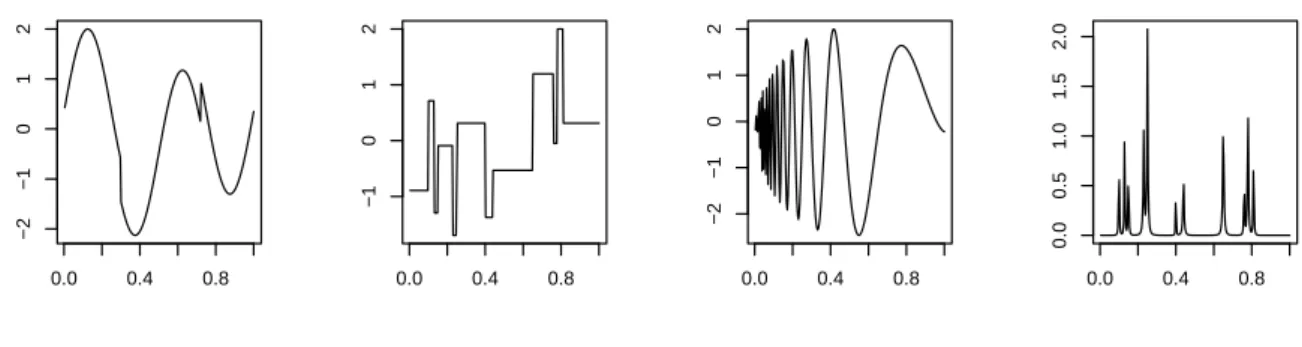
The four test signals introduced byDonoho and Johnstone(1994) were considered in the functional part f:

• theHeavisinefunction, for a smooth function, combination of sinusoidal functions, • theBlocksfunction, for a piecewise constant function,

• theDopplerfunction, for a high frequency signal

• and theBumpsfunction for a function presenting localised high variations.

These functions are given in Figure1.

0.0 0.4 0.8 −2 −1 0 1 2 (a) 0.0 0.4 0.8 −1 0 1 2 (b) 0.0 0.4 0.8 −2 −1 0 1 2 (c) 0.0 0.4 0.8 0.0 0.5 1.0 1.5 2.0 (d)

Figure 1: Functional part of the generalized partially linear model. Figure (a) corresponds to the Heavisinefunction, Figure (b) to theBlocksfunction, Figure (c) to theDopplerfunction and Figure (d) to theBumps function.

We will more precisely study the estimation quality for

• a Gaussian distribution; observations areyi ∼ N(ηi,σ2), withσ2=φ,

• a Binomial distribution; observations are yi such that yi×m ∼ B(µi,m)withm = φ−1and the logit link function,i.e.µi = ₁₊exp_exp(η₍i_η)_i),

• a Poisson distribution; observations areyi ∼ P(µi), with the link function,i.e.µi =exp(ηi),

To conclude with respect to the quality of estimation, we will give the mean value of the squared error for the parameterβ, notedMSE_βwhich is the empirical mean ofSEβ = ∑_jp=1(bβj−βj)2. For the nonparametric part, we will evaluate the average mean squared error, noted AMSEf, which is the empirical mean of MSEf = 1_n∑ni=1

b

fn(ti)− f0(ti) 2

. To evaluate the global estimation quality, we will also compute a global average mean sqared error AMSE, empirical mean of MSE=∑(1 n∑ n i=1 X_iTbβ_n+ bfn(ti)−XiTβ0−f0(ti) 2 .

All results were obtained on 500 simulations with the same covariatesXi and the same functional parts f. A maximal number ofκ =200 iterations was taken and the tolerance value defined above was equal toδ=10−10when applying the algorithms. The Daubechies’s wavelets base with a filter length of 8 was chosen. Concerning the kernel estimators, the Biweight kernel was used, with a bandwidth varying from 0.005 to 0.05 with a step of 0.005. The splines estimators were computed with a smoothing parameter varying from 0.2 to 0.7 with a step of 0.05. Kernel bandwidths and splines smoothing parameters are chosen by minimizing the GCV score.

3.2.1 Preliminary study: choice of the threshold level

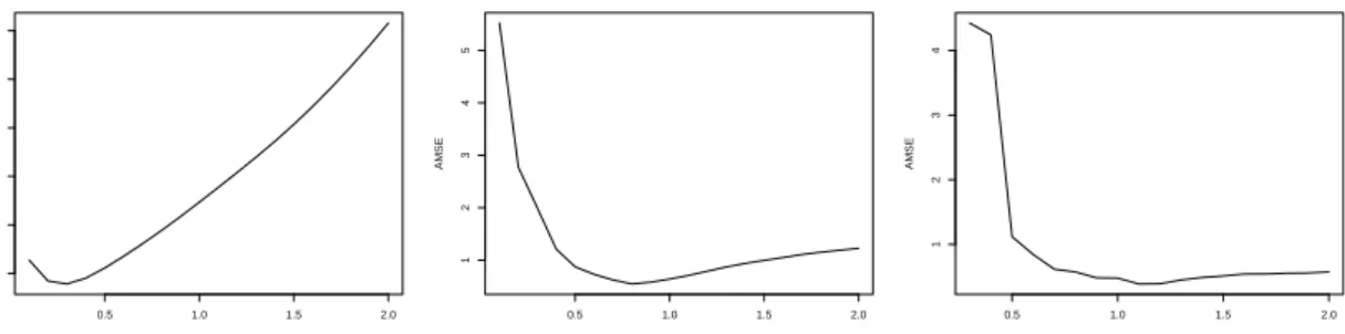
The asymptotic behaviour of the estimators only defines the threshold level λ up to a constant. Yet, numerical implementation needs to determine the exact threshold levelλin the algorithm. In practice, one can see it has an important impact on the quality of estimation. Figure2 gives the evolution of the AMSE with respect to the threshold level in the GPLM with different distributions. One can observe that the threshold levels attaining the minima are very different among the distribution.

With a Gaussian distribution, following Donoho et al (1995), we choose λ = p2φlog(n). This choice overevaluates the optimal threshold level in many cases but is the most often encountered in practice.

Binomial distribution. Due to homogeneity reasons, it seems well-adapted to fix a threshold level of the formλ = c′₀pφlog(n), whereφcorresponds to the dispersion parameter in distribution (1)

0.5 1.0 1.5 2.0 0.02 0.04 0.06 0.08 0.10 0.12 (a) AMSE 0.5 1.0 1.5 2.0 1 2 3 4 5 (b) AMSE 0.5 1.0 1.5 2.0 1 2 3 4 (c) AMSE

Figure 2: Evolution of the functional AMSE with respect to the threshold level in a generalized functional model with the Heavisine function. Figure (a) corresponds to a Gaussian distribution with the dispersion parameterφ = 0.05, Figure (b) to a Binomial distribution with the dispersion parameterφ=0.05 and Figure (c) to a Poisson distribution. Calculations were done on 50 data sets of sizen= 28.

andc′₀denotes a positive constant.

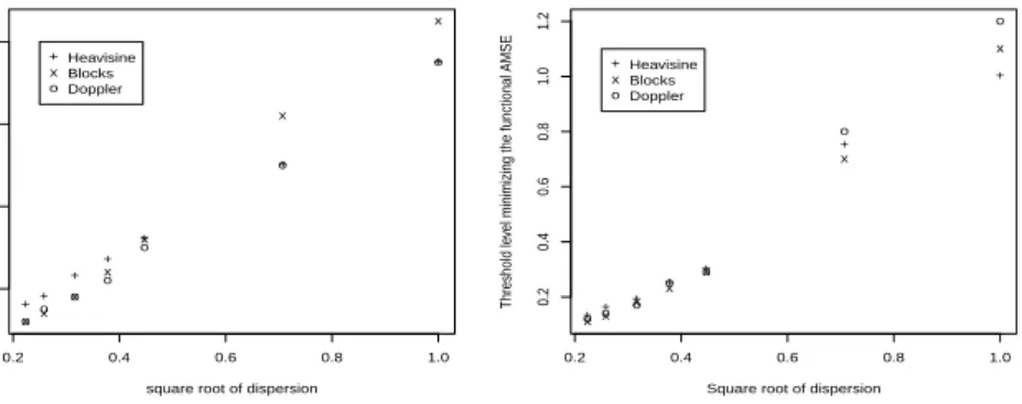
To ensure this conjecture in a Binomial setup, we plot the optimal threshold obtained for different value of the Binomial parameterm. The study was done on a generalized functional model (GFM) and on a GPLM. Figure 3 confirms that the chosen form seems appropriate. Linear fittings are given in Table1. The Bumpssignal was not considered during this preliminary step because the evaluation of the minima in the functional AMSE leads to a threshold level which clearly over-smoothes the function.

Table 1: Numerical indexes for the regression of the threshold level that minimizes the functional AMSE with respect to pφlog(n) with a Binomial distribution. Calculations were done on 100 samples of sizen=28_.

Generalized functional model Function Heavisine Blocks Doppler R2coefficient 0.999 0.992 0.988 constantc₀′ 0.306 0.269 0.258

Generalized partially linear model Function Heavisine Blocks Doppler R2coefficient 0.997 0.999 0.988 constantc′₀ 0.273 0.257 0.259

++ + + + + + 0.2 0.4 0.6 0.8 1.0 0.2 0.4 0.6 0.8 (a)

square root of dispersion

Threshold le

vel minimizing the functional AMSE

xx x x x x x oo o o o o o + x o Heavisine Blocks Doppler ++ + + + + + 0.2 0.4 0.6 0.8 1.0 0.2 0.4 0.6 0.8 1.0 1.2 (b)

Square root of dispersion

Threshold le

vel minimizing the functional AMSE

x x x x x x x o o o o o o o + x o Heavisine Blocks Doppler

Figure 3: Evolution of the threshold minimizing the functional AMSE when estimating the Heavisine, Blocks and Doppler functions in a Binomial setup, with respect to √φ. In a GFM on Figure (a) and in a GPLM in Figure (b). Calculations were done on 100 samples of sizen=28. The linear fitting is coherent provided the R2 coefficients. The constant c′₀ obtained by linear fitting is varying with respect to the simulated samples, but the observed variations are small. The mean value is 0.306 and the standard deviation is 0.019. The conjecture of a uniform constant seems acceptable. We therefore choose to take the value c′₀ = 0.3 in the following for Binomial distributions. Note that due to the central limit theorem, one would have expected to takec′₀=√2 for large values of the parameter m, but our simulation study shows that this would lead to an oversmoothing for small values ofm.

Note all the calculations were done with a fixed sample size n = 28. To better evaluate the form of the optimal threshold in practice, one could also study the evolution of the threshold level with respect to the sample sizen.

Poisson distribution. Estimation in a Poisson functional model has been more intensively

explored. Note thatSardy et al(2004) propose a threshold level. The main drawback is that the level given depends on the estimated function. Yet, the choice is based on an universal large deviation inequality which does not seem to be well-adapted in this procedure. Indeed, due to the iterative interpretation of the estimation, the inhomogeneity of the variance of the observations is taken into account within the estimation.

Recently, Reynaud-Bouret and Rivoirard (2010) have developed a procedure based on wavelet hard-thresholding estimation for Poisson regression. In their estimation the thresholding step is defined directly and not through a penalization procedure like here. The authors then present a detailed numerical study showing the high instability of the optimal threshold level with respect to the estimated function.

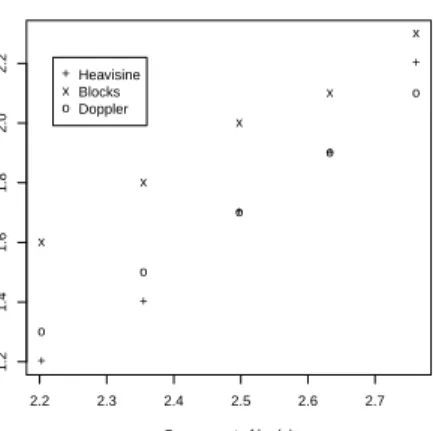
In our procedure, we observe that the optimal threshold level does not vary significantly with respect to the estimated function; this can bee seen on Figure4which represents the evolution of the threshold level which minimizes the AMSE with respect to plog(n) in a Poisson functional regression. The minima can clearly be identified in the generalized functional model but they are much more approximative in a partially linear context. Consequently, we prefer not to take them into account in our study.

+ + + + + 2.2 2.3 2.4 2.5 2.6 2.7 1.2 1.4 1.6 1.8 2.0 2.2

Square root of log(n)

Threshold le

v

el minimizing the functional AMSE

x x x x x o o o o o + x o Heavisine Blocks Doppler

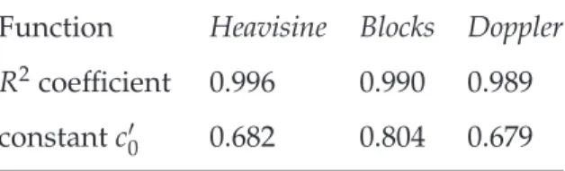
Figure 4: Evolution of the optimal threshold with respect toplog(n)with a Poisson distribution in a Generalized functional model. Calculations were done on 100 samples for each value ofn. As the theoretical result is asymptotic, we should study larger values of the sample size n. According to the results in Table 2, one may choose a constant approximatively equal to 0.72 in a functional model and in a GPLM. We therefore choose to take the valuec′₀=0.72 in the following for Poisson distribution.

Table 2: Numerical indexes for the regression of the threshold level that minimizes the functional AMSEwith respect toplog(n)with a Poisson distribution. Calculations were done on 100 samples for each size ofn.

Generalized functional model Function Heavisine Blocks Doppler R2coefficient 0.996 0.990 0.989 constantc′₀ 0.682 0.804 0.679

Remark: In a Gaussian or a Binomial regression, one may need the dispersion parameter φ.

Actually in literature, it is classically estimated at each iteration by

φ(k) = 1 n n

∑

Due to the bad quality of this estimator in GPLM, we prefer to consider in this paper that the dispersion parameter is known. In a Gaussian model, Gannaz (2007b) proposed an efficient QR-based estimator for φ. It would be interesting to explore whether it could be extended to generalized models.

3.2.2 Example 1: Gaussian distribution

Example 1 deals with a Gaussian model. The Gaussian distribution implementation is not a novelty for this estimation procedure, and we refer toChang and Qu(2004),Fadili and Bullmore(2005) and Gannaz(2007b) for detailed studies on simulated or real values data. We briefly consider this case in order to have a comparison base for other distributions.

The signal-to-noise ratio (SNR) of a signal is defined as the norm of the ratio of the mean value with respect to the standard deviation. In GPLM the SNR for the nonparametric part, notedSNRf and

the SNR for the linear part of the model, notedSNR_β, are respectively equal to SNR2_f = 1 n n

∑

∑

With a high SNR, say approximatively 5, one can expect a good quality of estimation, while with a small value, like 1, the quality of estimation cannot be satisfying.

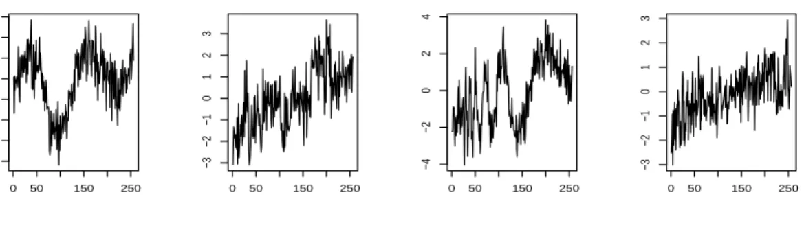
Example 1 considered Gaussian observations with a variance φ = σ2 = 0.05. An example of simulated observations obtained in this example are given in Figure5. TheSNR_β for the linear regressor is approximatively equal to 3.8 with each target signals and the functional SNRf is respectively equal to 5.5 for theHeavisine function, 3.6 for theBlocks function, 5.8 for theDoppler function and 0.97 for theBumpsfunction. Except for theSNRf of theBumpssignal, the SNRs are high and we expect a good quality in estimation.

0 50 150 250 −4 −3 −2 −1 0 1 2 3 (a) 0 50 150 250 −3 −2 −1 0 1 2 3 (b) 0 50 150 250 −4 −2 0 2 4 (c) 0 50 150 250 −3 −2 −1 0 1 2 3 (d)

Figure 5: An example of a simulated data set in Example 1, with theHeavisinefunction in Figure (a), the Blocksfunction in Figure (b), theDoppler function in Figure (c) and the Bumpsfunction in Figure (d).

In order to evaluate if the quality observed for the wavelets based procedure is due or not to the presence of the linear part, we give in Table3theAMSEfor an usual functional regression model yi ∼ N(f(ti), 0.05),i.e.without linear part.

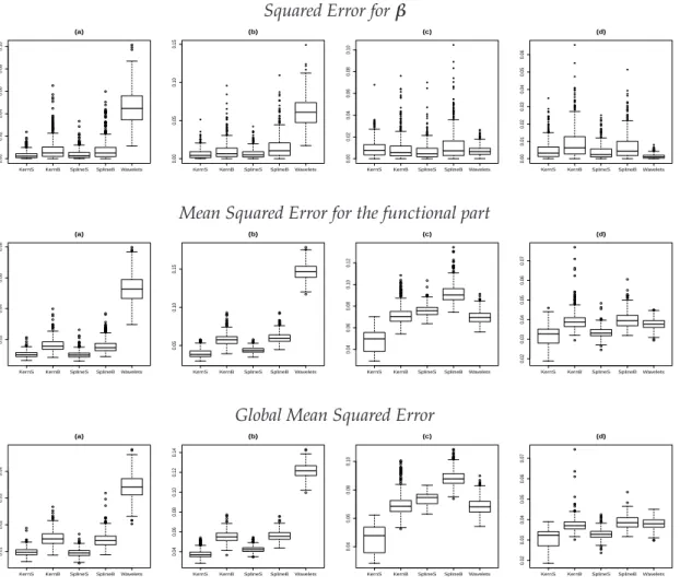
All the numerical measures for each estimation procedure are given in Table 4. This Table is completed by the boxplots of the squared errors for the linear part MSE, the mean squared errors for the functionnal part and the global mean squared errors, in Figure7.

Table 3: Measures of quality the wavelet estimator over the 500 simulations in an gaussian functional regression model yi = f(ti) +εi with n = 28, εi following a gaussian distribution N(0, 0.05)and differents functions f.

f Heavisine Blocks Doppler Bumps

AMSEf 0.03411 0.01061 0.698 0.0403

The quality indexes show that the wavelets based estimators do not perform as well as the kernel or spline based methods when estimating the functionsHeavisineorBlocks. The quality is also lower for the linear part when considering such functional parts. Yet, we can see with Table3that even in a functional model the AMSE for wavelets estimators are lower than those obtained by kernel or splines estimators. It would be interesting in such contexts to study if a GCV step improves the quality of the wavelets-based procedure.

Concerning the simulations with theDoppleror theBumpsfunctions, we can see that wavelets-based procedure is satisfactory. The best AMSE for the functional part is given by the kernel method with Speckman algorithm but then wavelets give results comparable with the others methods. Note also that the boxplots illustrate that wavelets lead to a more stable estimation of the linear part.

We can remark that in this example, whatever the functional part is, the backfitting procedures perform worse than the Speckman algorithms. The kernel based estimator with Speckman algorithm gives in many cases the best quality indexes. If results are close to the ones of splines estimator with Speckman algorithm for Heavisine and Blocks signals, it is more performant for DopplerandBumpsnonparametric parts.

Finally, to illustrate the visual quality of our functional estimators, we give in Figure 6 the estimated functions for one simulation with each test functions. As expected, the estimates tends to oversmooth the functions (see Donoho and Johnstone (1994)). Other threshold levels were proposed in literature but not tested here. The peaks in the Bumpssignal are not all identified by our procedure but this is coherent with the small SNR.

0.0 0.2 0.4 0.6 0.8 1.0 −2 −1 0 1 2 (a) 0.0 0.2 0.4 0.6 0.8 1.0 −1 0 1 2 (b) 0.0 0.2 0.4 0.6 0.8 1.0 −2 −1 0 1 2 (c) 0.0 0.2 0.4 0.6 0.8 1.0 0.0 0.5 1.0 1.5 2.0 (d)

Figure 6: An example of estimation of the nonparametric part in Example 1, with the Heavisine function in Figure (a), theBlocksfunction in Figure (b), theDoppler function in Figure (c) and the Bumpsfunction in Figure (d). Dots lines corresponds to the true functions and plain lines to their estimate.

Squared Error forβ

KernS KernB SplineS SplineB Wavelets

0.00 0.02 0.04 0.06 0.08 0.10 (a)

KernS KernB SplineS SplineBWavelets

0.00

0.05

0.10

0.15

(b)

KernS KernB SplineS SplineB Wavelets

0.00 0.02 0.04 0.06 0.08 0.10 (c)

KernS KernB SplineS SplineBWavelets

0.00 0.01 0.02 0.03 0.04 0.05 0.06 (d)

Mean Squared Error for the functional part

KernS KernB SplineS SplineB Wavelets

0.02

0.04

0.06

0.08

(a)

KernS KernB SplineS SplineBWavelets

0.05

0.10

0.15

(b)

KernS KernB SplineS SplineB Wavelets

0.04 0.06 0.08 0.10 0.12 (c)

KernS KernB SplineS SplineBWavelets

0.02 0.03 0.04 0.05 0.06 0.07 (d)

Global Mean Squared Error

KernS KernB SplineS SplineB Wavelets

0.01

0.02

0.03

0.04

(a)

KernS KernB SplineS SplineBWavelets

0.04 0.06 0.08 0.10 0.12 0.14 (b)

KernS KernB SplineS SplineB Wavelets

0.04

0.06

0.08

0.10

(c)

KernS KernB SplineS SplineBWavelets

0.02 0.03 0.04 0.05 0.06 0.07 (d)

Figure 7: Boxplots of the MSE in Example 1, with theHeavisine function in Figures (a), theBlocks function in Figures (b), the Doppler function in Figures (c) and the Bumps function in Figures (d). KernSandKernBstand for the kernel procedures respectively with Speckman algorithm and Backfitting algorithm, andSplineSandSplineBstands for the splines procedures respectively with27

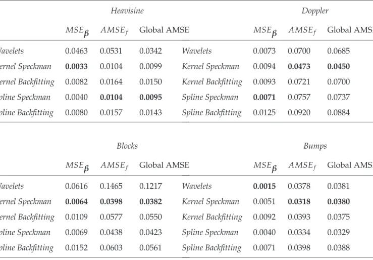
Table 4: Measures of quality the estimates over the 500 simulations in Example 1 withn = 28and

φ=0.05. Lowest values are in bold face type.

Heavisine

MSE_β AMSEf Global AMSE Wavelets 0.0463 0.0531 0.0342 Kernel Speckman 0.0033 0.0104 0.0099 Kernel Backfitting 0.0082 0.0164 0.0150 Spline Speckman 0.0040 0.0104 0.0095 Spline Backfitting 0.0080 0.0157 0.0143 Blocks

MSE_β AMSEf Global AMSE Wavelets 0.0616 0.1465 0.1217 Kernel Speckman 0.0064 0.0398 0.0382 Kernel Backfitting 0.0109 0.0577 0.0550 Spline Speckman 0.0069 0.0438 0.0423 Spline Backfitting 0.0152 0.0603 0.0561 Doppler

MSE_β AMSEf Global AMSE Wavelets 0.0073 0.0700 0.0685 Kernel Speckman 0.0094 0.0473 0.0450 Kernel Backfitting 0.0093 0.0721 0.0700 Spline Speckman 0.0071 0.0757 0.0737 Spline Backfitting 0.0125 0.0920 0.0884 Bumps

MSE_β AMSEf Global AMSE Wavelets 0.0015 0.0378 0.0381

Kernel Speckman 0.0051 0.0318 0.0380

Kernel Backfitting 0.0092 0.0393 0.0375 Spline Speckman 0.0040 0.0334 0.0329 Spline Backfitting 0.0071 0.0398 0.0388

3.2.3 Example 2: Binomial distribution

In Example 2, we consider a Binomial distribution: observations Yi are such that Yi ×m are independently drawn from Binomial distributionsB(µi,m)with the parametermequal tom= φ−1. The link function considered is the logistic. The mean is thus equal to

µi =

exp(XT_i β₀+ f0(ti)) 1+exp(X_iTβ₀+ f0(ti))

.

The logistic link makes sense if the canonical parameterη(·)belongs to the interval[−4, 4], as one can see for example page 28 ofFahrmeir and Tutz(1994). Consequently, to get a SNR of order 3 one may choose a parameter min the binomial distribution equal approximatively to 50. This choice is not adapted for real data applications, especially when the binomial regression corresponds to a classification problem.

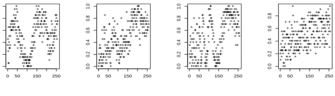
Due to this remark, we choose here to make a compromise and to apply the algorithm with a parameter m equal to 20, which corresponds to 21 classes. This choice is not coherent with a classification problem but allows to consider much reasonable SNRs. The observations of a simulated sample are represented in Figure 8. The results for this example are summarized in Table5. Figure9gives the boxplots of the squared error obtained by the five methods considered.

+ + + + + + + + + + + + + + + + + + + + + + + + ++ + + + + + + +++ + + + + + + + + + + + + ++ + + + + + + + + + + + + + + + + + + + + + ++ + + + + + + + + + + + + + + + + + + + ++++ + + ++ + ++ + + + + ++ + + + ++ + ++ + + + + + + + + + + + + + + + + + + + + + + + + + + + + ++ + + + + + + + + + ++ + + + + + + + + + + + + + ++ + + + + + + + +++ + + ++ + + + + + + + ++ + + + + + + + + + + + + + + + + + + + + + + + + + + + + + + + + + + + + ++ + + + + + + + + + + + + + + + + ++ + + + + + 0 50 150 250 0.0 0.2 0.4 0.6 0.8 1.0 (a) + + + + + + + + ++ + ++ + + + + + + + + + + + + ++ + + + + + + + + + + + + + + + + + + + ++ + + + + + + + + + + + + ++ + + + + + + + + + + + + + + + + + + + + + + ++++ + + ++ + + + + + + + + + + + + +++ ++ + + + + + + + + + + ++ + + + + + + + + + + + + + + + + + + + + + + + + + + + + + + + + + + + + + + + + + + + + + + + + ++ + + + + + + ++ + + + + + + + ++ + + + + + + + + + + + + + +++ ++ + + + + + + + + + + + + + + + + + + + + + + + + ++ + + + + + + + + + + ++ + + + + + + +++ + + + 0 50 150 250 0.0 0.2 0.4 0.6 0.8 1.0 (b) + + + + + + + + + + + + + + + + + + + + + + + + + + + + + + + + + ++ + + + + + + + + + ++ + + + + + + + + + + + + + +++ + + + + + + + + + + + + + + + + + + + + ++ + + + + + + + + + + + + + + + + + + + + + + ++ + + + + + + + + + + + + + + + + + + + + + ++ + + + + ++ + + + + + + + + + + ++ + + + + ++ + + + + + + + + + + + + + + + + + + + + + + + + + + + + + + + + + ++ + ++ + ++++ + + + + + + + + + + + + + + + + + + + +++ + + + +++ + + + + + + + + + + + + + + + + + + + + + + + + + + + + + + 0 50 150 250 0.0 0.2 0.4 0.6 0.8 1.0 (c) + + + + + + + + + + + + + + + + + + + + + + + + + + + + + + + ++ + + + + + + + + + + + + + + + + + + + + + + ++ + + + + + + + + + + + + + + + + + + + + + + + + + + + + + + + + + + + + + + + + + + + + + + + + ++ + + + ++ + + + + + + + + + + + + + + + + ++ + ++ + + + + + + + + + + + + + + + + + + + + + + + + + + + + + + +++++ + + + + + + + + + + + + + + + + + + ++ + + + + + + + + + + + + + + + + + + + + + + + + + + + + + + + + + + + + + + + + + + + + + + + + + + + + + + + + + + + + + + + + + + + + 0 50 150 250 0.0 0.2 0.4 0.6 0.8 (d)

Figure 8: An example of the observations obtained on a simulation in Example 2, with theHeavisine function in Figure (a), theBlocksfunction in Figure (b), theDoppler function in Figure (c) and the Bumpsfunction in Figure (d).

Contrary to Example 1 where the kernel procedures over-performed the splines in the functional part estimation, it appears in Example 2 that the splines-based procedures give better quality indexes. The case of the Doppler signal is the most relevant of this fact. On the same way, the

Table 5: Measures of quality the estimates over the 500 simulations in Example 2 withn = 28and

φ=1/20.

Heavisine

MSE_β AMSEf Global AMSE Wavelets 0.1538 0.1172 0.0691 Kernel Speckman 0.0305 0.0640 0.0621 Kernel Backfitting 0.1134 0.0932 0.0830 Spline Speckman 0.0244 0.0349 0.0339 Spline Backfitting 0.0294 0.0350 0.0355 Blocks

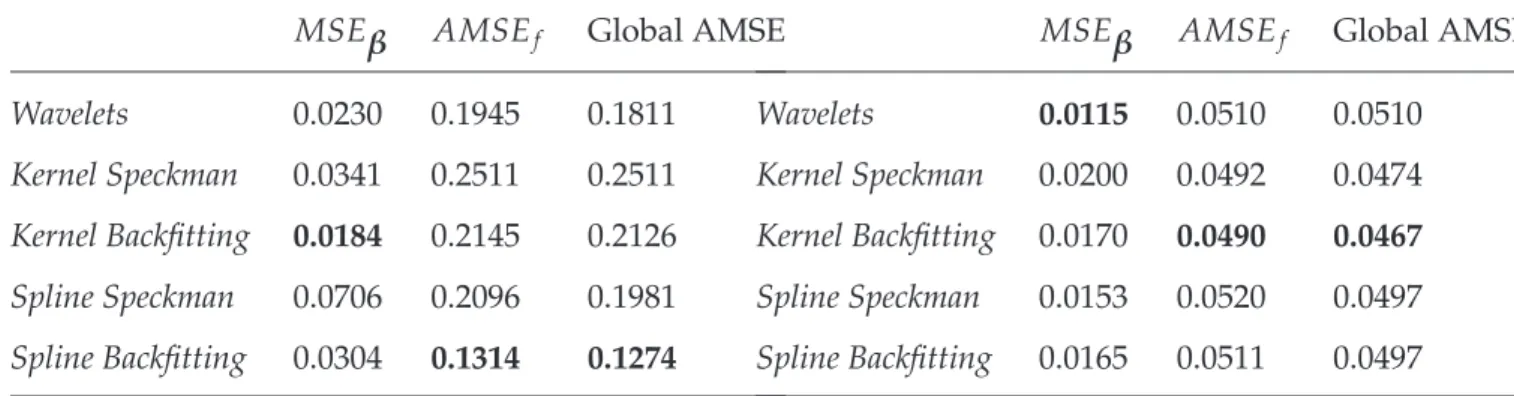
MSE_β AMSEf Global AMSE Wavelets 0.0230 0.1945 0.1811 Kernel Speckman 0.0341 0.2511 0.2511 Kernel Backfitting 0.0184 0.2145 0.2126 Spline Speckman 0.0706 0.2096 0.1981 Spline Backfitting 0.0304 0.1314 0.1274 Doppler

MSE_β AMSEf Global AMSE Wavelets 0.0159 0.1801 0.1846 Kernel Speckman 0.0427 0.03662 0.3737 Kernel Backfitting 0.0421 0.3486 0.3488 Spline Speckman 0.0444 0.2060 0.1914 Spline Backfitting 0.0233 0.1780 0.1762 Bumps

MSE_β AMSEf Global AMSE Wavelets 0.0115 0.0510 0.0510

Kernel Speckman 0.0200 0.0492 0.0474 Kernel Backfitting 0.0170 0.0490 0.0467

Spline Speckman 0.0153 0.0520 0.0497 Spline Backfitting 0.0165 0.0511 0.0497

differences which appeared in Example 1 between backfitting algorithms and Speckman algorithms are no more observed. The backfitting algorithm even give better results, except with theHeavisine signal.

Concerning the wavelets scheme, one can see that with the Heavisine functional part, it still has the worst quality for the linear and the functional part. Yet the difference with others methods is less important by comparison with the Gaussian distribution. With the others nonparametric test functions, the squared errors of the wavelets-based estimators are nearly the same as splines-based estimators and they lead to better quality indexes than kernel procedures.