Development and application of quantitative image analysis for preclinical MRI research

Al-Mubarak, Haitham (2020) Development and application of quantitative image analysis for preclinical MRI research. PhD thesis.

https://theses.gla.ac.uk/81370/

Copyright and moral rights for this work are retained by the author

A copy can be downloaded for personal non-commercial research or study,

without prior permission or charge

This work cannot be reproduced or quoted extensively from without first

obtaining permission in writing from the author

The content must not be changed in any way or sold commercially in any

format or medium without the formal permission of the author

When referring to this work, full bibliographic details including the author,

title, awarding institution and date of the thesis must be given

Enlighten: Theses https://theses.gla.ac.uk/ [email protected]

HAITHAM FAROOQ IBRAHIM AL-MUBARAK

B.Sc., M.Sc.

SUBMITTED IN FULFILMENT OF THE REQUIREMENTS FOR

THE DEGREE OF

Doctor of Philosophy

Institute of Neuroscience and Psychology

College of Medical, Veterinary and Life Sciences

II The aim of this thesis is to develop quantitative analysis methods to validate MRI and improve the detection of tumour infiltration. The major components include a description of the development the quantitative methods to better validate imaging biomarkers and detect of infiltration of tumour cells into normal tissue, which were then applied to a mouse model of glioblastoma invasion. To do this, a new histology model, called Stacked In-plane Histology (SIH), was developed to allow a quantitative analysis of MRI.

Validating imaging biomarkers for glioblastoma infiltration

Cancer can be defined as a disease in which a group of abnormal cells grow uncontrollably, often with fatal outcomes. According to (Cancer research UK, 2019), there are more than 363,000 new cancer cases in the UK every year, an increase from the 990 cases reported daily in 2014-2016, with only half of all patients recovering.

Glioblastoma (GB) is the most frequent and malignant form of primary brain tumours with a very poor prognosis. Even with the development of modern diagnostic strategies and new therapies, the five-year survival rate is just 5%, with the median survival time only 14 months.

Unfortunately, glioblastoma can affect patients at any age, including young children, but has a peak occurrence between the ages of 65 and 75 years. The standard treatment for GB consists of surgical resection, followed by radiotherapy and chemotherapy. However, the infiltration of GB cells into healthy adjacent brain tissue is a major obstacle for successful treatment, making complete removal of a tumour by surgery a difficult task, with the potential for tumour recurrence.

Magnetic Resonance Imaging (MRI) is a non-invasive, multipurpose imaging tool used for the diagnosis and monitoring of cancerous tumours. It can provide morphological, physiological, and metabolic information about the tumour. Currently, MRI is the standard diagnostic tool for GB before the pathological examination of tissue from surgical resection or biopsy specimens. The standard

III biological functions, pathogenic processes or pharmacological responses to therapeutic interventions (Atkinson et al., 2001). In fact, when new MRI methods are proposed as imaging biomarkers of particular diseases, it is crucial that they are validated against histopathology. In humans, such validation is limited to a biopsy, which is the gold standard of diagnosis for most types of cancer. Some types of biopsies can take an image-guided approach using MRI, Computed Tomography (CT) or Ultrasound (US). However, a biopsy may miss the most malignant region of the tumour and is difficult to repeat. Biomarker validation can be performed in preclinical disease models, where the animal can be terminated immediately after imaging for histological analysis. Here, in principle, co-registration of the biomarker images with the histopathology would allow for direct validation. However, in practice, most preclinical validation studies have been limited to using simple visual comparisons to assess the correlation between the imaging biomarker and underlying histopathology.

First objective (Chapter 5): Histopathology is the gold standard for assessing non-invasive imaging biomarkers, with most validation approaches involving a qualitative visual inspection. To allow a more quantitative analysis, previous studies have attempted to co-register MRI with histology. However, these studies have focused on developing better algorithms to deal with the distortions common in histology sections. By contrast, we have taken an approach to improve the quality of the histological processing and analysis, for example, by taking into account the imaging slice orientation and thickness. Multiple histology sections were cut in the MR imaging plane to produce a Stacked In-plane Histology (SIH) map. This approach, which is applied to the next two objectives, creates a

IV validate imaging biomarkers.

Second objective (Chapter 6): Glioblastoma is the most malignant form of primary brain tumour and recurrence following treatment is common. Non-invasive MR imaging is an important component of brain tumour diagnosis and treatment planning. Unfortunately, clinic MRI (T1W, T2W, CE-T1, and FLAIR) fails to detect regions of glioblastoma cell infiltration beyond the solid tumour region identified by contrast enhanced T1 scans. However, advanced MRI techniques such as Arterial Spin Labelling (ASL) could provide us with extra information (perfusion) which may allow better detection of infiltration. In order to assess whether local perfusion perturbation could provide a useful biomarker for glioblastoma cell infiltration, we quantitatively analysed the correlation between perfusion MRI (ASL) and stacked in-plane histology. This work used a mouse model of glioblastoma that mimics the infiltrative behaviour found in human patients. The results demonstrate the ability of perfusion imaging to probe regions of low tumour cell infiltration, while confirming the sensitivity limitations of clinic imaging modalities.

Third objective (Chapter 7): It is widely hypothesised that Multiparametric MRI (mpMRI), can extract more information than is obtained from the constituent individual MR images, by reconstructing a single map that contains complementary information. Using the MRI and histology dataset from objective 2, we used a multi-regression algorithm to reconstruct a single map which was highly correlated (r>0.6) with histology. The results are promising, showing that mpMRI can better predict the whole tumour region, including the region of tumour cell infiltration.

V

1.7.1 Surgery 7

1.7.2 Radiotherapy 8

1.7.3 Chemotherapy 9

1.8 Preclinical GB models 10

Chapter 2: The theory of magnetic resonance imaging 2.1 Background of MRI 13 2.2 MRI principle 13 2.2.1 Resonance 16 2.2.2 RF pulse 17 2.3 Relaxation 17 2.3.1 T1 relaxation 18 2.3.2 T2 relaxation 19 2.3.3 T2 * relaxation 19 2.4 Gradients 20

2.5 Gradient and spin echo sequences 22

2.6 MR signal 24

2.7 k-space 25

2.8 Main parts of MRI scanner 27

2.9 Applications of relaxation 28

2.9.1 T1 Weighted imaging 29

2.9.2 T2 Weighted imaging 29

2.10 Diffusion 30

2.10.1 Diffusion encoding 31

2.10.2 Apparent diffusion coefficient 33

2.10.3 Diffusion tensor imaging 34

VI

2.13 Perfusion 38

2.14 Perfusion weighted magnetic resonance imaging 39

2.14.1 Contrast Enhanced T1 40

2.14.2 Dynamic contrast enhanced 41

2.14.3 Dynamic susceptibility contrast MRI 41

2.14.4 Arterial spin labelling 41

2.15 Application of ASL 45 Chapter 3: An introduction to image analysis techniques 3.1 Introduction 47

3.2 MRI pre-processing 47

3.2.1 Retrieve data 47

3.2.2 Normalization 47

3.2.3 Sensitivity of surface coil 48

3.2.4 ADC map calculation 49

3.2.5 Skull stripping 49 3.2.6 Filter 50 3.3 MRI Post-processing 52 3.3.1 Segmentation 52 3.3.2 Registration 55 3.4 Histology 58 3.4.1 Pre-processing histology 60 3.4.2 Post-processing histology 61 3.5 Validation Measurement 61 3.5.1 Visual assessment 61

3.5.2 Dice similarity coefficient 61

3.5.3 ROC analysis 62

3.5.4 Reproducibility 63

Chapter 4: Material and experimental methods 4.1 Animal study design 66

4.1.1 Mice and tumour implantation 66

4.1.2 Experimental design 67

4.1.3 MRI acquisition 68

VII

5.6.1 Tumour volume measurement via single-section histology (SSH)

83

5.6.2 Determining optimal number of histology sections for SIH maps 84

5.6.3 SIH to MRI registration quality 86

5.6.4 Volumetric assessment of SIH maps 87

5.6.5 Towards voxel-by-voxel assessment 89

5.7 Conclusion 91

Chapter 6: Quantitative histopathological assessment of perfusion MRI as a marker of GB infiltration 6.1 Introduction 93

6.2 Tumour region of interest selection 95

6.3 Statistical analysis 96

6.4 Results 96

6.4.1 A marginal infiltration of mouse model 96

6.4.2 PWI detects more extensive regions of tumour infiltration than clinic MRI 98 6.4.3 Relationship between perfusion and invasion in tumour margin 101 6.4.4 Perfusion variation as a marker of tumour cell infiltration 102

6.5 Discussion 104

6.6 Limitations 107

VIII

data to detect GB infiltration

7.1 Introduction 109

7.2 Regression analysis models 112

7.3 MRI pre-processing 113

7.4 Statistical analysis 115

7.5 Results 116

7.5.1 Visual analysis 118

7.5.2 Pearson correlation 118

7.5.3 Volumetric analysis of tumour 119

7.5.4 Probability density function analysis 121

7.6 Discussion 123

7.7 Conclusion 125

7.8 Future directions 125

Chapter 8: General conclusion 8.1 Discussion 127

8.1.1 Limatations 131

8.2 Conclusion 131

8.3 Future directions 133

Appendix A Published peer reviewed articles during PhD study 135

IX

Figure 1.5: Three types of radiation therapy target volume GTV ,CTV and PTV.

9 Figure 1.6: Glioblastoma tumour cells derived from human biopsies

injected within the mouse brain’s healthy tissue. 10

Figure 2.1: The magnetic field causes the nucleus to precess at the

Larmor frequency. 14

Figure 2.2 Spin align with and without external magnetic field present. 15 Figure 2.3: Schematic diagram showing the separation of energy levels

with and without an external magnetic field.

15 Figure 2.4: Schematic diagram showing the net magnetisation parallel to

the external magnetic field during a 90° pulseand dephase.

17 Figure 2.5: T1 recovery and T2 decay curves. 18 Figure 2.6: A T2* signal decay after an RF pulse. 19 Figure 2.7: Gradient (Gz) as a linear function of main magnetic field. 20 Figure 2.8: Shows principles of slice selection. 21 Figure 2.9: In vivo brain MR images acquired in (A) Axial (B) Sagittal (C)

Coronal.

22 Figure 2.10: Time diagram of basic gradient-echo sequence. 23

X

Figure 2.12: k-space diagram. 26

Figure 2.13: The major parts of an MR scanner and electrical

components. 28

Figure 2.14: Example of T1W image of mouse brain. 29 Figure 2.15: Example of T2W image of mouse brain. 30 Figure 2.16: Free diffusion particle moving from two points. 31 Figure 2.17: The Stejskal-Tanner diffusion sequence. 31 Figure 2.18: Mono-exponential of diffusion signal decay of water in MR. 33 Figure 2.19: Illustration of isotropic and anisotropic diffusion. 34 Figure 2.20: Represented eigenvalues of isotropic and anisotropic

diffusion.

35 Figure 2.21: Example of DWI with a malignant brain tumour in mouse. 36 Figure 2.22: Example of ADC map of brain tumour in mouse. 36 Figure 2.23: Example of FA image of brain tumour in mouse. 37 Figure 2.24: Illustration of blood-brain barrier components. 37 Figure 2.25: Difference of flow between normal and abnormal tissue. 39 Figure 2.26: Injection of contrast agent (Gd) in mouse-tail. 40 Figure 2.27: Shows T1W brain image pre and post injection ,and

subtraction after injection of Gd contrast.

XI

Figure 3.3: T2W brain image before and after skull stripping. 50 Figure 3.4: Applying anisotropic diffusion filter. 52 Figure 3.5: Applying Gaussian Mixture Model on mouse brain. 55 Figure 3.6: Linear, rigid ,rotation and affine transformation models. 56 Figure 3.7: Comparison 2D histograms with and without rotation. 57 Figure 3.8: Block diagram of the histology process. 59 Figure 3.9: Example of H&E stains imaging. 59 Figure 3.10: Example of HLA stains imaging. 60 Figure 3.11: Visual assessment using checkerboard after co-registration

of MRI with histology images.

61 Figure 3.12: The interaction of two regions A and B. 62 Figure 3.13: Diagram of comparison of two regions true positive (TP),

true negative (TN), false positive (FP) and false negative (FN) regions.

XII

Regions of vascular cuffing by invading tumour cells are enlarged.

Figure 4.2: Experimental protocol of first study. 67 Figure 4.3: Experimental protocol of second study. 67 Figure 4.4: MRI Biospect 7T scanner and equipment used in the

experiment. 68

Figure 4.5 : Example of MR images of first experiment in week12. 70 Figure 4.6: Example of MR images of second experiment weeks 15 and

17.

71 Figure 5.1: Effect of cutting angle (φ) on MRI and histology with

comparison of slice thickness.

78 Figure 5.2: The cutting of histology sections were guided by 0.5 mm thick T2WHistology with slice thickness comparsion.

78 Figure 5.3: Simplified diagram of the image processing pipeline leading

to the production of 3D matrices after combining MRI modalities and SIH data.

79 Figure 5.4: Co-register of three HLA sections to construct at SIH map

and 3D matrix.

81 Figure 5.5: Examples of histology sections for both HLA and H&E stains

and tumour volume error comparison between sections. 83 Figure 5.6: SIH maps generated using several sections of HLA with

tumour volume comparison. ROC analysis to evaluate the ability of 5 sections SIH maps to probe the tumour volume.

85 Figure 5.7: Example of non-rigid co-registration of histology with T2W

MRI and Checkerboard validation. 86

Figure 5.8: Volumetric analysis for T2W five individual histology sections and SIH.

88 Figure 5.9: Power calculation between SIH and T2W for two different

single slice groups (A) section SSH1 (B) section SSH2.

89 Figure 5.10: Scatter plots between T2W, ADC MRI modalities and

histology.

90 Figure 6.1: T2W and CE-T1 (pre and post injection) at week 12 with Ki67

immunohistochemistry on slices.

XIII

modalities.

Figure 7.2: Schematic showing the voxel by voxel analysis method used to generate a single tumour map.

111 Figure 7.3: Examples of Linear regression, Quadratic regression, and

Cubic regression fitting.

113 Figure 7.4: Image processing pipeline to create regression maps. 114 Figure 7.5: Comparison of original MR images in different regression

maps.

118 Figure 7.6: Pearson correlation comparison between regression maps

and SIH. 119

Figure 7.7: Volumetric analysis of tumour between QRM and CRM regression maps and SIH map.

120 Figure 7.8: Comparison of volumetric analysis between multiple

regression maps and SIH 120

Figure 7.9: Comparison of volumetric analysis between QRM, CRM and SIH.

121 Figure 7.10: Comparison of normalised probability density function (PDF)

between CRM and SIH for whole brain.

122 Figure 7.11: Comparison between QRM, CRM and SIH. 123

XIV

Table 7.1: The multi-regression coefficients (bi) of IRM, QRM and CRM.

XV

XVI

Throughout my studies I received a tremendous amount of support from

multiple people. I would like to take this opportunity to thank them for

helping me to achieve my PhD.

First, I give thanks to Allah for helping me and giving me the knowledge,

patience, and strength to successfully complete this PhD. I would like to

acknowledge the advice and guidance of my advisors, Dr. William

Holmes and Dr. Antione Vallatos. They have been more than mentors

in guiding me throughout my entire time in the in INP/MVLS at University

of Glasgow and have played a pivotal role in this project. They were

always there to offer help and support and were understating of the

problems that arose throughout my writing. They provided the required

background and experiential knowledge for the work. Also, I would like

to thank Dr. Jozien Goense, Dr. John Foster, Dr. Joanna Birch, and

Giacinta Frisillo for their help and feedback.

I am sincerely thankful for the support of my family members, without

whom I wouldn’t have been able to finish my thesis.

No words can

express my gratitude and thanks to my wife for caring for my family while

I was busy with my studies, and for her patience and endless support

and sacrifices. Also, I would like to thank and appreciate my sponsor,

The Ministry of Higher Education and Scientific Research in Iraq, for

their administrative and financial support.

Finally, I would like to thank my colleagues, Abdulrahman, Mohammed

and Samantha

for their encouragement and support. In addition, I would

like to thank all the staff of INP/MVLs, Lindsay, James, Linda, and Conor

for providing me with essential information about the thesis that helped

a lot in planning and pacing my work.

XVII

XVIII

1_{H Hydrogen atoms}

3D Three dimensional 5-ALA 5-Amiinolevulinic acid A Cross-section area

ADC Apparent Diffusion Coefficient ASL Arterial Spin Labelling

b Magnitude of diffusion encoding gradients B1 RF magnetic field

BBB Blood-Brain Barrier

B0 The main magnetic field-7 Tesla

Blocal Local magnetization

C Curie

CA Contrast Agent

CAD Computer Aided Diagnosis CBF Cerebral Blood Flow

CBV Cerebral Blood Volume CE-T1 Contrast Enhanced T1 cMRI Clinic MRI

CNS Central Nervous System CRM Cubic Regression Map CSF Cerebrospinal Fluid

CT Computed Tomography

CTV Clinical Target Volume CV Coefficient of Variation D Diffusion coefficient DC Direct Current

DCE Dynamic Contrast-Enhanced Dice Dice Similarity Coefficient

DICOM Digital Imaging and Communication in Medicine DSC Dynamic Susceptibility Contrast

DTI Diffusion Tensor Imaging DWI Diffusion Weighted Imaging EM Expectation Maximization EPI Echo Planner Imaging

f Frequency

FA Fractional Anisotropy

FCM Fuzzy C-Means

FID Free Induction Decay

FITC-dextran Fluorescein Isothiocyanate–dextran FLAIR Fluid Attenuated Inversion Recovery FN False Negative

FOV Field Of View FP False Positive G Gradient amplitude

Gd-DTPA Gadolinium-Diethylene Triamine Penta-Acetic

GB Glioblastoma

Gd Gadolinium

GE Gradient Echo

GM Grey Matter

XIX

LRM Linear Regression Map

mbASL Multiple Boli Arterial Spin Labelling mpMRI Multiple parametric MRI

Mcontrol Control Image

MD Mean Diffusivity MI Mutual Information mI Spin quantum number

Mlabel Labelled Image

Mpost Image post injection with Gd

Mpre Image pre injection with Gd

M0 Net equilibrium magnetisation

MRA Magnetic Resonance Angiograph MRI Magnetic Resonance Imaging MTT Mean Transit Time

MSME Multi Slice Multi Echo

Mxy Transvers component of the net magnetisation

NC3RS UK government policy of Replacement, Refinement and Reduction

Mz Longitudinal component of the net magnetisation

Ndown Number of spins in lower energy level

NMR Nuclear Magnetic Resonance

Nup Number of spins in upper energy level

PBS Phospate Buffered Sline

PET Positron Emission Tomography PTV Planning Target Volume

PWI Perfusion Weighted Imaging QRM Quadratic Regression Map

RARE Rapid Acquisition with Relaxation Enhancement RF Radio Frequency

RGB Red, Green and Blue

ROC Receiver Operating Characteristic ROI Region Of Interest

S Signal

SE Spin Echo

SIH Stacked In-plane Histology SNR Signal to Noise Ratio SOC Standard Of Care

XX

SSH Single Section of Histology STD Standard Deviation

t Time

T Temperature

T1 Longitudinal relaxation time

T1W T1Weighted

T2 Transvers relaxation time T2* _{Effective T2 relaxation time}

T2W T2Weighted TE Echo Time TI Inversion Time TM Transformation Model TMZ Temozolomide TN True Negative tp Period of time TP True Positive TR Repetition Time US Ultrasound

VEGF Vascular Endothelial Growth Factor Vmax Maximum Tumour Volume

Vmin Minimum Tumour Volume

VOI Volume Of Interest

ω0 Larmor frequency

WHO World Health Organisation

WM White Matter

Δ Observation time

ΔE Energy difference

δ Duration of the gradient pulse

λ Parallel diffusivity

λ1, λ2, λ3 The first, second and third eigenvalues of diffusion tensor

μ Magnetic moment

Σi Covariance matrix

XXI Gilmour, L., Holmes, W. M., Chalmers, A. J., (2018), J Magn Reson Imaging: 1-12, Doi: 10.1002/jmri.26580.

• Changes an apparent diffusion coefficient across the macroscopic tumour margin correlate with novel tissue measures of infiltration in a preclinical glioblastoma Model (Conference abstract).

Thompson G., Vallatos A., Birch J., Al-Mubarak H., Gallagher L., Gilmour L., Waldman A., Holmes W., and Chalmers A., Neuro Oncol, 2018, 20: i15., Doi: 10.1093/neuonc/nox238.066.

XXII

• National 3R’s Prize 2018 by the Animal Welfare and Ethical Review Board (AWERB),UK.

XXIII

• British Neuro-Oncology Society Annual Conference, 21-23 June

2017, Edinburgh, UK.

1- Probing glioblastoma infiltration into healthy tissue by magnetic resonance perfusion imaging: a quantitative MRI evaluation, oral presentation, session OS-22F.

A. Vallatos, J.L. Birch, H. Al-Mubarak, L. Gallagher, L. Gilmour, J.E. Foster, A.J. Chalmers, W.M. Holmes.

2- Changes in Apparent Diffusion Coefficient across the Macroscopic Tumour Margin Correlate with Novel Tissue Measures of Infiltration in a Preclinical Glioblastoma Model, Abstract. Neuro-Oncology, Volume 20, Issue suppl_1, 1 January 2018, Page i15, https://doi.org/10.1093/neuonc/nox238.066.

Gerard Thompson, Antoine Vallatos, Joanna Birch, Haitham Al-Mubarak, Lindsay Gallagher, Lesley Gilmour, Adam Waldman, William Holmes, Anthony Chalmers.

3- BBB permeability as a magnetic resonance imaging biomarker for low glioblastoma infiltration, Abstract, Neuro-Oncology, Volume 20, Issue suppl_1, 1 January 2018, Page i25 , https://doi.org/10.1093/neuonc/nox238.115.

Antoine Vallatos, Joanna Birch, Haitham Al-Mubarak, Lindsay Gallagher, Lesley Gilmour, Anthony Chalmers, William Holmes.

• 25th _{Annual ISMRM Meeting and Exhibition, 22-27 April 2017,}

Haonolulu, USA.

Multi-parametric MRI of glioblastoma invasion quantitative evaluation using histological stacks, Poster,2929.

H. Al-Mubarak, A. Vallatos, L. Gallagher, J.L. Birch, L. Gilmour, J.E. Foster, A.J. Chalmers, W.M. Holmes.

• ESMRMB Magnetic Resonance Materials in Physics, Biology and

Medicine, Congress, October 19 – 21, 2017, Barcelona, Spain.

Detecting of Glioblastoma Invasion Cells Using Multi-parametric MRI and Quantitative Assessment with in-plane Histology, Oral presentation, 325.

H. Al-Mubarak, A. Vallatos, J. Birch, L. Glmour, L. Gallagher, J. Mullin, A. Chalmers, W. Holemes.

XXIV

• Annual ISMRM–ESMRMB Meeting, 16-21 June 2018, Paris, France.

1- Detecting glioblastoma invasion using multi-parametric MRI and

quantitative assessment with in plane histology,e-poster, 3831.

H. Al-Mubarak, A. Vallatos, L. Gallagher, J.L. Birch, L. Gilmour, J.E. Foster, A.J. Chalmers, W.M. Holmes.

2- Perfusion MRI as a marker of glioblastoma infiltration into health tissue, e-poster, 6026.

A. Vallatos, H. Al-Mubarak, L. Gallagher, J.L. Birch, L. Gilmour, J.E. Foster, A.J. Chalmers, W.M. Holmes.

3- Apparent diffusion coefficient correlates with histological tumour burden at infiltrating margins of a prclinical glioblastoma model, e-poster, 6526.

Gerard Thompson, Antoine Vallatos, Joanna Birch, Haitham Al-Mubarak, Lindsay Gallagher, Lesley Gilmour, Adam Waldman, William Holmes, Anthony Chalmers.

4-Quantitative Assessment of MRI Biomarkers Using Non-Rigid Registration of Stacked in-Plane Histology: Application in a Mouse G7 Tumour Model,e-poster, 4858.

H. Al-Mubarak, A. Vallatos, L. Gallagher, J.L. Birch, L. Gilmour, J.E. Foster, A.J. Chalmers, W.M. Holmes.

• The Sinapse Annual Scientific Meeting, 25 June 2018, Edinburgh, UK.

1- Stacked in plane histology for quantitative MRI assessment: Application to an infiltrative brain tumour model, oral presentation, O6.

H. Al-Mubarak, A. Vallatos, L. Gallagher, J.L. Birch, L. Gilmour, J.E. Foster, A.J. Chalmers, W.M. Holmes.

2- Perfusion as a marker of brain tumour infiltration into healthy brain tissue: a quantitative MRI evaluation, oral presentation, O13.

H. Al-Mubarak, A. Vallatos, L. Gallagher, J.L. Birch, L. Gilmour, A.J. Chalmers, W.M. Holmes.

• 24th _{Annual ISMRM Scientific Meeting of the British Chapter, 24-26}

September 2018, Oxford, UK.

1- Investigating How to Optimally Combine Multimodal MRI Data to Better Identify Glioblastoma Infiltration, oral presentation, O16.

H. Al-Mubarak, A. Vallatos, L. Gallagher, J.L. Birch, L. Gilmour, J.E. Foster, A.J. Chalmers, W.M. Holmes.

2- Stacked In-plane Histology for Quantitative Assessment of MRI Markers: Application to an Infiltrative Brain Tumour Model, Power pitch, PP24.

H. Al-Mubarak, A. Vallatos, L. Gallagher, J.L. Birch, L. Gilmour, J.E. Foster, A.J. Chalmers, W.M. Holmes.

1

1

Chapter 1

General Introduction to Imaging and

Treatment of Brain Tumours

2 aggressiveness. Benign tumours grow very slowly, have distinct borders, seldom infiltrate into the surrounding tissue, and can usually be completely removed by surgery and without recurrence (Louis et al., 2016). Malignant tumours on the other hand, grow rapidly, are difficult to remove completely by surgery and infiltrate to the surrounding normal tissues or metastasis (Hejmadi, 2013).

1.2

The brain anatomy

The brain is the most complex organ in the human body and is part of the Central Nervous System (CNS). It is surrounded by the skull and consists of Grey Matter (GM), White Matter (WM) and Cerebrospinal Fluid (CSF). GM consists of neural cell bodies, neuropil, glial cells, synapses, and capillaries (Mescher, 2016). WM contains myelinated axons. CSF is a clear fluid which exists in the ventricles and surrounds the brain and spinal cord.

1.3

Brain tumours

There are several types of brain tumours, such as glioblastoma, astrocytoma, pituitary adenoma, acoustic neuroma, meningioma, oligodendroglioma, haemangioblastoma, CNS lymphoma, and others (Hattingen and Pilatus, 2016, Mescher, 2016). Brain tumours can be classified into two categories: primary and secondary. Primary brain tumours arise from the cells inside the brain. Secondary brain tumours are the result of metastases. This occurs when tumour cells separate from a primary tumour site and migrate to the brain through the blood system or the lymphatic system (Cuddapah et al., 2014, Weinberg, 2007).

3

1.4

Glioma

Gliomas are the most common form of malignant primary brain tumours and arise

de novo from glial cells and their progenitors in the brain. Until recently, glioma

tumour cell classification was based on microscopic examination of tumour specimens by neuropathologists. However, since 2016, the World Health Organization (WHO) has classified tumours of the Central Nervous System (CNS) by integrating both classical histology features (morphological appearance) and molecular biomarkers that are based on the specific group’s molecular and gene expression profile (Louis et al., 2016).

Gliomas have a variety of grades and degrees of aggressiveness that can be divided into low-grade benign gliomas (grade I and II) or high-grade malignant gliomas (grade III or IV).

Grade I tumours are different from the three other grades. Typically, tumour cells are relatively unchanged compared to normal cells, and proliferate very slowly and rarely infiltrate into the surrounding tissue. Complete surgical resection can usually be achieved due to the distinct borders between a normal brain and tumour tissue (Louis et al., 2016).

Grade II tumour cells do not look like normal cells. The tumour grows slowly and often progress into a higher-grade tumour despite therapy. Studies show that the tumours return in the form of highly invasive tumours (grade IV) 5 to 10 years after the original diagnosis and subsequent treatments (Bogdanska et al., 2017).

Grade III (Higher malignant) tumours are invasive tumours that share common characteristics with grade IV tumours. The tumour cells invade healthy neighbouring brain tissue and after this are more likely to become rapidly dividing cells, but the tumours contain no dead cells at their centre (necrotic). The tumour tends to recur after surgery (Lacroix et al., 2001).

Grade IV is a glioblastoma, which is a very aggressive tumour; they are heterogeneous, grow very fast, build new blood vessels, contain dead cells (necrosis) in the centre, and complete surgical resection is not achievable (De vleeschouwer, 2017).

4 One of the hallmarks of high-grade glioma is the ability of a single tumour cell or small groups to infiltrate adjacent normal tissue (Krakhmal et al., 2015). The invasion of tumour cells can occur in several ways (Fig.1.1), i.e., through the parenchyma (dashed green square), along vasculature (dashed blue square), via white matter tracts (dashed purple rectangle), or in the leptomeningeal space, dashed red rectangle (de Gooijer et al., 2018, Zagzag et al., 2008). The leptomeningeal space is the space between the arachnoid membrane and pia mater that is filled with cerebrospinal fluid and contains the large blood vessels that supply the brain. In fact, glioma cells are locally invasive and very rarely metastasise.

5

Figure 1.1: Invasion of tumour cells in to normal brain tissue. Four different routes of invasion have been described: (1) via the brain parenchyma, (2) perivascular space, (3) white matter tracts, and (4) leptomeningeal space. Adapted from (de Gooijer et al., 2018).

The primary routes of invasion by glioma cells are by migrating through the perivascular space surrounding blood vessels or along white matter tracts. Claes et al. (2007) reported that high-grade glioma cells usually use the same routes of migration that are travelled by immature neurons. The invasion of tumour cells mostly happens along white matter fibers and extend to corpus callosum into the contralateral hemisphere.

1.6

Medical imaging of GB

There are several techniques to evaluate tumour progression, diagnosis, and monitoring of GB. The standard imaging techniques used to diagnose and monitor brain tumours are X-ray Computed Tomography (CT) and Magnetic Resonance Imaging (MRI). Other techniques have been used such as Positron Emission Tomography (PET), and Single-Photon Emission Computed Tomography, SPECT,(De vleeschouwer, 2017).

6

Figure 1.2: Shows the difference in spatial resolution between CT and MRI in mouse. MRI is superior in regards to the detail of the image and the tumour can be clearly seen. Image from (Karellas and Thomadsen, 2016).

MR images are generally classified into two types, clinic and advanced imaging. Clinic MRI (cMRI) images are qualitative, whereas advanced MRI methods provide quantitative or semi-quantitative measurements. These are discussed in chapter 2.

The standard MRI sequences that are used to detect GB in the clinic are T2-Weighted, T1-T2-Weighted, Contrast Enhanced T1 and Fluid-attenuated inversion recovery. These clinic MRI (cMRI) modalities are useful to discriminate between brain tumours and normal tissue, although they are not able to detect the infiltration of tumour cells into the normal tissue (Sternberg et al., 2014). Several studies show that cMRI cannot detect the invasion of tumour cells beyond oedema (Swanson et al., 2002, Baldock et al., 2013, Vallatos et al., 2018a). Clinic MR cannot detect the invasion of a low density of tumour cells because, the current limit for tumour cell detection by MRI is in range between 100-500 cells (Muja and Bulte, 2009, Heyn et al., 2005). For more details see Fig.1.3.

7

Figure 1.3: A theoretical distribution of tumour cell density represented by the smooth curve showing the tumour distribution extending beyond the region detected by T2W and beyond the region detected by CE-T1. Adapted from (Konukoglu et al., 2010).

1.7

Treatment of glioblastoma

The current Standard of Care (SOC) for glioblastoma treatment is maximal surgical resection followed by radiotherapy and chemotherapy with for example Temozolomide (Jain, 2018). However, since glioblastoma tumour cells can infiltrate several centimetres beyond the treatment volume defined by standard CT or MRI (Tracqui, 1995) this can lead to tumour recurrence and regrowth.

1.7.1

Surgery

Surgical resection is the first choice for the treatment of GB. However, this treatment routine almost always fails to remove the tumour completely due to the aggressive, heterogeneous and infiltrative nature of this type of tumour (Lacroix et al., 2001). Complete surgical removal is not always possible, as it is difficult to distinguish the tumour from normal tissue and sometimes the tumour’s location is too near essential regions of the brain.

A significant development in oncology in recent years has been the use of fluorescence-guided surgery. The patient consumes a drink that enables surgeons during operation to target brain tumours accurately, by making cancer cells fluoresce pink. The liquid is called 5-Aminolevulinic Acid (5-ALA) that uses a fluorescent dye to make cancerous cells fluoresce under UV light (Fig.1.4 A,B).

8

Figure 1.4: (A) Shows the surgical location of a small glioblastoma. (B) After drink of exogenous 5-ALA dye, the tumour cells become fluorescent under UV light. This feature can identify tumour cells clearly and facilitates resection. Adapted from (Hattingen and Pilatus, 2016).

1.7.2 Radiotherapy

Radiation therapy is an effective method to attack tumour cells. The radiation dose applied to the tumour is dependent on its location and the radio-sensitivity of the surrounding tissue. X-rays and gamma rays are routinely used in radiation therapy to treat various cancers. Their deposited energy can kill cancer cells or cause genetic changes resulting in cancer cell death (Baskar et al., 2012). The standard fractionated intensity X-rays in three-dimensional radiotherapy is in a total dose of 60Gy in 30 daily fractions, every weekday over a period of six weeks (Caranci et al., 2012).

In conventional radiation therapy three types of target volume are chosen to radiate. Firstly, the Gross Tumour Volume (GTV) is the lesion as identified in a magnetic resonance imaging scan with CE-T1 contrast. Secondly, the Clinical Target Volume (CTV) is defined as GTV plus an expansion margin of 2cm where there may be infiltration of tumour cells. Thirdly, the Planning Target Volume (PTV) is represented by CTV plus an expansion margin of 1cm (Burnet et al., 2004).

Figure 1.5 shows these three volumes. This additional margin results in a PTV, which may often be four or more times the volume of the original GTV. Figure 1.5 provides an illustration of how large PTV is compared to GTV. Hence, PTV usually incorporates a large number of critical brain regions and applying radiation to

9 these regions can result in irreversible damage. The conventional approach of adding a 2cm Euclidean margin to the GTV to construct a PTV is based on limited scientific evidence (Pirtoli and Gravina, 2016, Hattingen and Pilatus, 2016).

Figure 1.5: The three types of target volume are chosen to radiate the tumour: GTV in black representing tumour centre. CTV is together with a 2cm margin forms the GTV to be radiated. The PTV represents summation of areas GTV and CTV with additional 0.7cm margin. Adapted from (Burnet et al., 2004).

1.7.3 Chemotherapy

Chemotherapeutic agents work by targeting and killing tumour cells. There are many different types of chemotherapy medication, however, they all work in a similar way. The current drug for glioblastoma is Temozolomide (TMZ). TMZ is a DNA alkylating agent, which causes irreversible DNA damage and ultimately cell death.

Due to the lack of effective treatments available to cure glioblastoma patients, new therapies have been investigated such as anti-angiogenic gene therapy to reduce the rapid vascularization of GB (Gerstner and Batchelor, 2012), immunotherapy to increase patient survival , and hormone therapy to inhibit GB growth and to induce apoptotic pathways (Altiok et al., 2011).

10 There are currently many mouse GB cell lines that that can be used to recapitulate features of GB such as the G7, U251, U87, and GL261 that have been implanted into the brains of mice (Jacobs et al., 2011). Each glioma model may provide varying similarities to human GB, which can be used to test the effectiveness of novel chemotherapeutic combinations (Jacobs et al., 2011). However, there are two reasons why studying tumour cell invasion is difficult. First, there are few animal models that show an invasive growth pattern. Second, there is a deficiency of high-grade glioma staining for pathologic analysis (Inoue et al., 2012).

Figure 1.6: Glioblastoma tumour cells derived from human biopsies capture many characteristic of the tumour. Tumour cells are injected within the healthy mouse brain. Adapted from (Perrin et al., 2019).

This has recently improved with the use of the resected human G7 Glioblastoma cell lines, which were donated to the University of Glasgow by Dr. Colin Watts of the University of Cambridge, UK (Carruthers, 2015). This model is rich with stem cells which are resistant to radiotherapy and chemotherapy (Gomez-Roman et al.,

11 2017) and has a pathology resembling human disease, including an infiltrative margin which is useful to test new MRI techniques.

13

2.1

Background of MRI

Rabi et al. (1938) were the first to describe Nuclear Magnetic Resonance (NMR) as a method for determining nuclear magnetic moments. After the Second World War, Bloch (1946) observed the ‘NMR’ phenomenon, as an radio frequency signal response to irradiating magnetic nuclei in a magnetic field with continuous-wave Radio Frequency (RF) . Cope and Damadian (1970) were the first to use NMR to scan living things and observed that different types of tissue (e.g. normal tissue and cancerous tissue) have different signal relaxation properties. Following this discovery, many research groups started developing techniques and systems for imaging (Mansfield and Grannell, 1973, Lauterbur, 1973), leading to modern MRI.

In clinical practice, MRI has become a very common imaging tool, used for diagnosis, surgical planning, and follow-up of treatment outcomes. Compared with CT, MRI has superior soft-tissue contrast. MRI is also non-invasive and, unlike CT, does not use ionising radiation, thereby benefitting patient health. It is currently understood that exposure to the static magnetic field in MRI does not lead to harmful biological effects. MRI can be safely repeated to observe changes in pathology, such as the progression of a disease or the impact of treatment.

2.2

MRI principle

NMR signals are generally obtained from nuclei with an odd mass number (active MRI nuclei), such as 1_H, 13_C, 23_{Na and} 31_{P (exceptions being} 2_{H and} 14_{N). These}

nuclei have a non-zero nuclear spin quantum number and a magnetic moment (). The interaction of the nuclei with the external magnetic field (B0) causes the

nuclear magnetic moments to align with and precess around the external magnetic field as shown in Fig.2.1.

14

Figure 2.1: The external magnetic field causes the nucleus to precess at the Larmor frequency

ω0. The Larmor frequency of precession is related to the strength of the magnetic field, B0.

The precession frequency is called the Larmor frequency

𝜔

𝜔

= −γB

Where 𝛾 is the gyromagnetic ratio, a constant specific to a particular nucleus (for

protons, 𝛾 = 42.58 MHz/T), and B0 the strength of the external magnetic field in Tesla.

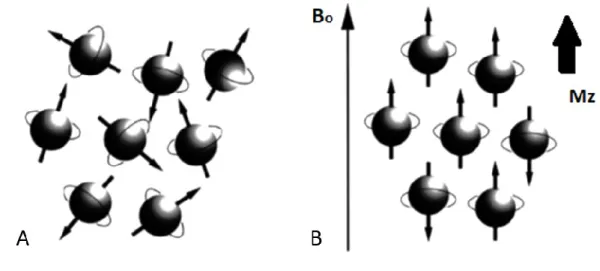
Generally, medical magnetic resonance imaging uses the signal from the nuclei of hydrogen atoms (1_{H) which contains a single proton. When no magnetic field is}

applied, the nuclear magnetic moments are oriented in random directions (Fig. 2.2A), and the net magnetisation (M0) will be zero. However, by applying an

external static magnetic field of B0, the nuclei will align along the flux lines of the

15

Figure 2.2 (A) With no external magnetic field present, spins rotate about their axes in a random direction. (B) In the presence of a magnetic field, slightly more spins align parallel to the main magnetic field, B, thus produce a net longitudinal magnetization, Mz. Note: diagram spins shown as perfectly aligned for convenience.

According to quantum mechanics, the number of possible orientations or energy states is determined by the nuclear spin quantum number, I. Hydrogen has a spin number of I= 1/2) and can adopt two possible spin states (2 I + 1). The low energy state (mI = +1/2), where the nuclear spin vector is in the same direction as the static field, is called spin-up. The high-energy state (mI = -1/2), where the nuclear spin vector is in the opposite direction, is called spin-down (Fig.2.3).

Figure 2.3: Schematic diagram showing the separation of energy levels of 1_{H with and without}

16

energy state (ΔE) is equal to:

∆E = hf = ħω = γħB

Where his Planck’s constant which is equal to 6.62×10-34 _m2_{Kg/s and ħ=h/2}

_π

M

=

cB

k

T

Where C is the Curie constant and M0 is the equilibrium net magnetisation.

2.2.1

Resonance

In physics, many systems are sensitive to the frequency of interactions, where the maximum energy transfer occurs at the resonance frequency. Excitation at this resonance frequency causes the system to enter an oscillating regime before returning to its initial state. NMR describes how protons aligned with the external magnetic field (B0) can be excited when a Radio Frequency (RF) pulse (‘excitation’

pulse B1), is applied at the same frequency as the precession frequency of the

nuclei.

In the presence of an external magnetic field (B0), the number of up and

17 RF pulse, the hydrogen nuclei absorb energy. This increases the number of high-energy (spin-down) nuclei (Fig.2.3) and creates phase coherence.

2.2.2

RF pulse

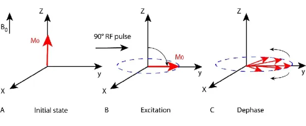
Magnetic resonance occurs when an RF pulse is applied at the same frequency as the Larmor frequency. For a group of nuclei, all the spins have the same phase after excitation by the RF pulse, resulting in a coherent transverse magnetization. In the presence of a receiver coil, the oscillating of the transverse magnetization induces an oscillating electric current in the receiver coil that can be measured. The dephasing due to the spins’ interaction during relaxation causes a loss of coherence and a decrease of transverse magnetization (Fig.2.4A-C).

Figure 2.4: Schematic diagram showing (A) The equilibrium net magnetisation (M0) parallel to

the external magnetic field (B0). (B) During the application of a 90° pulse, the M0 moves from

the z-axis to the xy-plane. (C) Spins lose coherence and dephase due to spin-spin relaxation.

2.3

Relaxation

Application of an RF pulse at the Larmor frequency will result in phase coherence and a net transverse magnetization (Mxy). The precessing transverse magnetization

gives rise to the MR signal in the receiver coil. However, the MR signal quickly disappears due to two independent processes that return the net magnetization back to the equilibrium state (M0). These two processes are spin-lattice relaxation

(T1 relaxation) and spin-spin relaxation (T2 relaxation), respectively (Weishaupt et al., 2006, McRobbie et al., 2006). For more details see Fig.2.5A-B.

18

Figure 2.5: (A) T1 recovery curve which represents exponentially increasing longitudinal magnetisation. (B) T2 decay curve that represents the decay of magnetisation in the transverse plane (Mxy) after switching off the RF pulse.

2.3.1

T1 relaxation

Spin-lattice relaxation (T1) refers to the time taken for energised nuclei (following a 90o _{pulse) to return to their equilibrium state. It is also known as the longitudinal}

relaxation time because, diagrammatically, it represents the time taken for the net magnetisation vector, M0, to recover along the B0 direction. The mechanism

underlying T1 relaxation is a transfer of energy from the nuclear spins to their surrounding lattice atoms (Guy and ffytche, 2005). The nuclei in the lattice are subject to vibrational and rotational motions, which create a separate, fluctuating local magnetic field (Blocal). This magnetic field can have frequency components

matching the Larmor frequency of the nuclei, which can drive transitions between energy levels, returning the system to equilibrium. The recovery is exponential, with an exponential time constant termed T1, equation 2.5, Fig.2.5A. The relaxation time is defined as the time taken for 63% of the longitudinal magnetisation to recover. T1 depends on the inherent characteristics of the tissue and the magnetic field strength. The longitudinal relaxation of the net magnetization vector, Mz, parallel to the external magnetic field can be described

by the equation:

M

= M

(1 − e

₎

Where t is time, M0 is the equilibrium net magnetization that depends on the

19

2.3.2

T2 relaxation

The z-component of the fluctuating local magnetic field Blocal, will add to the

static magnetic field B0, causing the local Larmor frequency to be time varying.

As individual spins experience a slightly different magnetic field, this results in dephasing and loss of transverse magnetisation (spin-spin relaxation). The decay is exponential, with an exponential time constant T2 (Fig.2.5B). T2 decay time is defined as the time taken for 63% of the transverse magnetisation to be lost. T2 also depends on the inherent characteristic of the tissue and the magnetic field strength and is usually faster than the corresponding T1 relaxation time. The transverse magnetization vector Mxy in the x-y plane can be described as:

M

= M

e

−t

T2 Equation 2.6

2.3.3

T2 * relaxation

After an RF pulse is applied, the Mz is tilted into the x-y plane, producing a signal

that is known as the Free Induction Decay (FID). The signal rapidly decays once the RF pulse is switched off due to parts per million level inhomogeneity in the static magnetic field, B0 (Fig.2.6).

Figure 2.6: After an RF pulse, T2* signal in rapid decay of resulting from inhomogeneities in the main magnetic field.

20

Figure 2.7: During a gradient pulse Gz where the magnetic field becomes a linear function of

position on the z axis. Bz = B0, at the centre of the magnet.

The gradient coils produce a linear variation of the magnetic field in the three directions, these are termed the x-gradient, Gx, the y-gradient, Gy, and the

z-gradient, Gz (Weishaupt et al., 2006). The magnetic field of these gradients can

be defined as follows:

G

=

∂B

∂x

,

G

=

∂B

∂y

, G

=

∂B

∂z

For example, the resultant magnetic field in the presence of a z-gradient can be expressed as:

21

B

= B

+ G

𝑧

Where B0 is the static magnetic field strength, Gz is a constant gradient measured

in T/m, and z is the spatial location within the object being imaged.

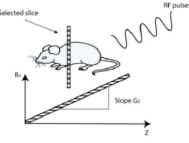
Magnetic field gradients can be used to select a slice for imaging. The slice- selection gradient is applied in the presence of an RF pulse whose bandwidth matches the precession frequency of spins in a thin slice that is to be imaged (Mougin, 2010), as shown in Fig.2.8.

Figure 2.8: Principles of slice selection are achieved by applying a one-dimensional, linear magnetic field gradient during the period that the RF pulse is applied.

A slice can be acquired with any orientation, but it is generally acquired in three orthogonal directions relative to the brain, namely, axial, sagittal, and coronal. Figure 2.9 illustrates MRI brain images taken in the three slice orientations.

22

Figure 2.9: In vivo MRI images acquired by 7T scanner showing (A) Axial (B) Sagittal, and (C) Coronal.

These magnetic field gradients are used to perform spatial encoding in two ways: frequency encoding and phase encoding. In frequency encoding, the gradient is applied to make the precession frequency linearly related to the spatial location (combining Equations 2.1 and 2.8):

ω(x) = ω

+ γG

𝑥

In phase encoding, the gradient is applied for a period of time (tp), during which

a phase is linearly accumulated along the phase encoding direction (z):

ϕ(y) = γG

yt

2.5

Gradient and spin echo sequences

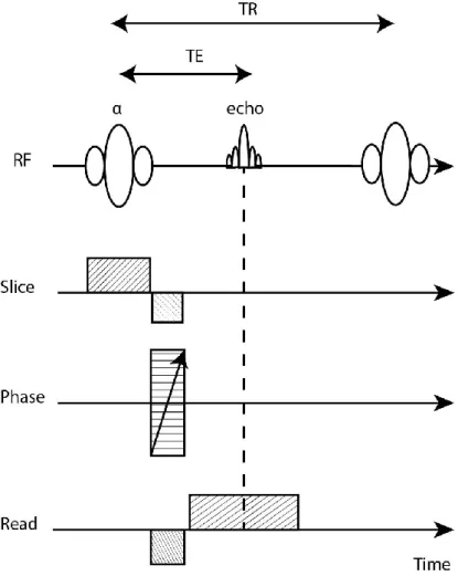
In MRI, signals can be generated using either Gradient-Echo (GE) or Spin-Echo (SE) sequences. In GE sequences (Fig.2.10), the RF pulse is set to produce a magnetisation rotation angle, called the flip angle (α), of less than 90o _{which is}

combined with short TEs and TRs. After the RF pulse, a negatively pulsed frequency-encoded gradient is immediately applied, causing rapid dephasing of the spins. A second frequency-encoded gradient with in opposite polarity is then applied, causing the spins to rephase. This is termed a gradient-echo. The signal obtained in this type of sequence depends on T2*, which is a fast decay following

23 the RF pulse. The time needed to produce an echo is shorter than that compared with SE sequences.

Figure 2.10: Time diagram of the basic gradient-echo sequence produced by a single RF pulse in conjunction with a gradient reversal. Adapted from (McRobbie et al., 2006).

In the basic SE sequence (Fig.2.11), a 90o _{RF pulse is first used to excite the}

hydrogen nuclei. After a certain period of time, during which the spins dephase naturally, an additional 180o _{pulse is applied (Westbrook et al., 2011). Such a pulse}

causes a rephasing of the spins, which produces an echo after a period equal to the time lapse between the two pulses.

24

Figure 2.11: Time diagram of the basic spin-echo imaging sequence produced by pairs of radiofrequency pulses 90o _{and 180}o_{, respectively. Adapted from (McRobbie et al., 2006).}

TR is the repetition time (the time between two successive 90o _{RF pulses). TE is}

the echo time (the time between the 90o _{RF pulse and the centre of the}

spin-echo).

2.6

MR signal

RF excitation creates a net ‘in-plane’ magnetisation Mxy, the precession of which

induces a signal in the receiver coil. The MRI signal can be expressed mathematically as follows:

s ∝ exp(i

𝜙

)

Where

𝜙

𝜙 =

25 Inputting equation 2.1 into equation 2.11 resulting in,

s ∝ exp(iγBt)

Where B external magnetic field and (t) time. In the rotating frame, while applying a gradient Bz(x)= Gx.x, the MRI signal is expressed as,

s ∝ e

2.7

k-space

The Cartesian coordinates of the reciprocal space vector, k, are termed k-space (Fig.2.12). K space is a spatial frequency domain that contains the digitised complex signals received during an MRI scan (Westbrook et al., 2011). Each point in k-space contains both the magnitude and the phase of the measured signal samples recorded in k-space, which can be transformed into a magnetic resonance image by using Fourier transform (Yankeelov et al., 2012). The signal detected by the receiver during an MRI scan is an oscillating circularly polarised magnetic field which can be separated into real and imaginary components. Two different image types can be generated. Magnitude images are most commonly generated by taking the modulus of the real and imaginary data, as in equation 2.15. Phase images are generated by taking the complex argument of the data, as in equation 2.16. Conventional MR is viewed in the magnitude image, while the phase image can be used to investigate flow.

Magnitude = √real

_{+ imaginary}

26

Figure 2.12: The analogue to digital conversion creates complex data points that are stored in a Cartesian grid called k-space, named after the reciprocal space vector k. Magnitude and phase images are generated by manipulation of the real and imaginary parts of the signal.

The frequency encoded (kx) and phase encoded (ky) in k-space are expressed as:

k

=

1

2π

γG

. t

k

=

1

2π

γG

. t

Integrating the signal for the whole sample, gives the total signal S(x,t). Equation 2.19 shows the Fourier relationship between the MRI signal and the spin density ().

S(x, t) = ∫

𝜌(𝑥)

+∞ −∞

27

2.8

Main parts of MRI scanner

In general, an MRI scanner includes the flowing elements:

1- The main magnet, which is commonly a coil made of superconducting wire immersed in liquid Helium, which carries a high electric current to generate a strong, stable, spatially uniform magnetic field B0 ,(Kenneth W. Fishbein).

2- A shim system containing coils carrying a small current that are used to compensate for the inhomogeneity of the main magnetic field (B0).

3- A gradient system consisting of three separate gradient coils, to produce linear gradients in the magnetic field in the x-, y-, and z-directions. These gradients are driven by powerful Direct Current (DC) amplifiers.

4- RF amplifier and RF transmit coil to produce the RF pulses.

5- Receiver coils (e.g. surface coil, head coil) used to receive signals from the body.

6- Various electrical components are controlling the scanner and the gradients, to create the MR images. For more details see Fig.2.13.

28

Figure 2.13: The major parts and electrical compounds of an MRI scanner are: the main magnet, gradient coils, shim system, RF transmitter and receiver, and the control computer.

2.9

Applications of relaxation

As discussed in section 2.3, the main relaxation processes are spin-lattice relaxation (T1 relaxation) and spin-spin relaxation (T2 relaxation). Relaxation produces the main form of contrast used in clinical MRI, as different tissues have different relaxation properties (Weishaupt et al., 2006).

29

2.9.1

T1 Weighted imaging

T1-weighting is obtained when both TE and TR are short. This procedure usually provides excellent contrast between fluids, water-based tissues, and fat-based tissues (McRobbie et al., 2006) . In the case of brain images, it presents a poor contrast between grey matter and white matter at 7 Tesla. In a T1W image, the CSF appears hypointense, while the brain tissues (GM and WM) appear with medium intensity, and fat has considerable hyper-intense values (Fig.2.14). Contrast agents can be intravenously injected, which alter the T1 of the tissue they perfuse (this is explained further in section 2.14.1).

Figure 2.14: Example of T1W image of mice with a G7 tumour model at 7 Tesla. Image parameters are TE=12.28 ms, TR=800 ms at a resolution of 176x176 pixels.

2.9.2

T2 Weighted imaging

Spin-spin relaxation is a much more rapid process, which refers to the time taken for coherent nuclei to dephase. Spin-spin relaxation is also known as transverse relaxation or T2 relaxation, it describes the reduction in the transverse magnetisation vector Mxy. Regarding the T2 values of brain tissues, this protocol

provides a good distinction between different parts of the brain e.g. GM, WM, CSF, and scalp fat. In regions with cerebrospinal fluid, e.g. the ventricles, the rapid molecular tumbling, results in the spin interactions occurring in shorter times with the slower loss of transverse coherence, which leads to a longer T2 time. Conversely, for more constrained structures such as the dense population of cells in the parenchyma, interaction and exchange with large molecules or solids result in faster loss of transverse coherence, which leads to shorter T2 times. Generally, in T2-Weighted images, fluids appear as hyperintensity, whilst water- and

fat-30

Figure 2.15: Example of T2W image of one nude mouse with G7 tumour type, TE= 47 ms, and TR = 4300 ms.

2.10

Diffusion

Robert Brown was the first to discover the random motion of pollen grains suspended in water while studying them through his microscope. Later, he demonstrated diffusive mixing by adding a few drops of ink to a glass of water, observing the ink spread (diffuse) and mix with the rest of the water (Moritani et al., 2005). This phenomenon is called ‘Brownian motion’. Later, Einstein described diffusion statistically by this equation:

< x

>= 6D∆

Where (

<x

_>)

proportional to the observation time (Δ), (Mukherjee et al., 2008) , Fig 2.16, and D is a constant, called the diffusion coefficient.

31

Figure 2.16: Free diffusing particle moving from two points, with displacement x, during observation time Δ.

2.10.1

Diffusion encoding

Stejskal and Tanner (1965) presented an NMR sequence sensitive to Brownian water motion. This sequence (Fig.2.17) is based on two gradients pulses (G) applied (in one spatial direction) on either side of 180o _{RF pulse. The presence of}

these gradients affects the spin-echo obtained at the end of the sequence. The greater the displacement of the spin along the gradient direction, the larger the dephasing and the greater the signal attenuation.

Figure 2.17: The Stejskal-Tanner sequence. The diffusion-encoding gradients are applied in two matched pulses. G gradient amplitude, δ gradient duration, Δ temporal separation of gradients.

During the first diffusion-encoding gradient, the spins accumulate a phase shift. If the spins are static, this phase shift is cancelled out by the second gradient, since

32

S (b) = S

exp

Where

b = γ

. δ

. G

. (Δ −

δ

3

)

Where 𝛾 is the gyromagnetic ratio (42.57 MHz/T for proton); G represents the

gradient amplitude; δ represents application time of the gradient and Δ the observation time, represents the separation between applied gradients.

The MRI signal that shows the diffusion displacement of spins in the direction of the gradient, is called the diffusion weighted signal. DW signals are not quantitative and the image obtained from these signals is called a Diffusion Weighted Image (DWI).

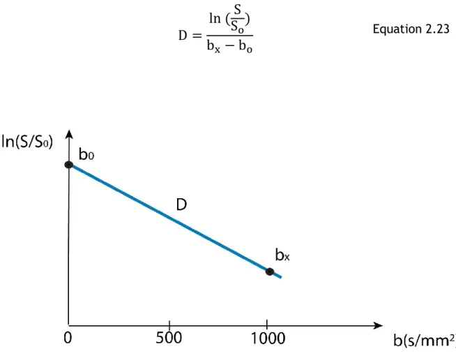
In order to calculate D, signal intensity needs to be measured with at least two b values. In a clinical setting, typically two (b) factors, 0 and 1000 s/mm2_{, are used.}

After performing a linear fit between ln (𝑆0/𝑆) and b, the diffusion coefficient D

can be calculated in a Region Of Interest (ROI) or voxel-by-voxel as the slope of linear regression (Mukherjee et al., 2008). For more detail see Fig.2.18.

33

D =

ln (

_S

S

)

b

− b

Figure 2.18: Mono-exponential signal decay curve of water signal in diffusion MR. The natural logarithm of the diffusion MR signal attenuation curve (ln (S/S0)) is shown against the b-value.

The slope of the line represents the diffusion coefficient.

2.10.2

Apparent diffusion coefficient

The measurement of the diffusion coefficients in three orthogonal directions (Dx,

Dy, Dz) can be used to generate an Apparent Diffusion Coefficient (ADC), which is

used to represent the quantitative measurement of the diffusion (mm2_{/s) in three}

directions.

ADC =

D

+ D

+ D

34

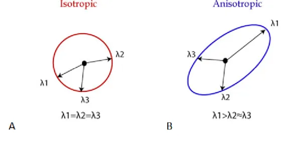
Figure 2.19: Illustration of isotropic diffusion and anisotropic restricted diffusion, with respective diffusion tensors. Adapted from (Mukherjee et al., 2008)

Diffusion tensor imaging (DTI) measurements in multiple directions of space (at least 6) can be used to produce a diffusion tensor for each voxel. The measures that can be extracted from the DTI dataset consist of the three eigenvalues (λ1, λ2 and λ3) that represent the diffusion coefficients measured along the 3

35

eigenvalues are of similar magnitude (λ1 ≈ λ2 ≈ λ3), Fig.2.20A, the diffusion of

water is not limited to any direction. However, restricted diffusion in a certain direction gives rise to diffusion anisotropy, Fig 2.2B, which can be quantified by the fractional anisotropy value (FA).

Figure 2.20: Representation of eigenvalues of isotropic and anisotropic diffusion of water.

FA can be computed (equation 2.25) as the ratio of the three eigenvalues, reflects the degree of directionality. FA has values between zero and one. FA=0 represents perfect isotropy (all eigenvalues are equal) and FA=1 corresponds to perfect anisotropy (diffusion in one direction only).

FA = √3 2

(λ1 − MD)2+ (λ2− MD)2+ (λ3 − MD)2

λ₁ + λ₂+ λ₃ Equation 2.25

Where MD is mean diffusivity:

MD =

λ

+ λ

+ λ

36

Figure 2.21: Example of DWI with a malignant tumour in a mouse brain. Acquired using b=1000 s/mm2_.

Several researchers have demonstrated the potential use of ADC as a non-invasive probe of tumour microstructure, which has motivated clinical and preclinical research to use ADC mapping to scan tumours (Moritani et al., 2005, Hecke et al., 2016). ADC measurement depends on the two b values, for example, measurements using low b values would be more sensitive to fast diffusion components such as blood, and measurement with high b values would be more sensitive to microstructure of the tissue (Drevelegas, 2011), Fig.2.22.

37 The magnitude and direction of diffusion of water molecules is determined by the geometry of the environment of the water spins. In grey matter, an FA value close to 0.2 is expected when little diffusion anisotropy is present, while in white matter, anisotropy is high and the FA values are expected to be nearer to 0.6, indicating a preferred direction of water diffusion, Fig.2.23.

Figure 2.23: Example of FA image map that is a quantitative measure of the micro-structural integrity and cohesion of white matter tracts.

2.12

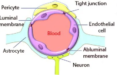
Blood brain barrier integrity

The Blood–Brain Barrier (BBB) was discovered in the late 19th _{century by Paul}

Ehrlich when he injected a dye into the bloodstream of a mouse. The dye infiltrated all tissues except the brain and spinal cord due to the existence of the blood–brain barrier. The blood–brain barrier is formed by endothelial cells of the blood vessel wall, astrocyte end-feet covering more than 90% of the blood vessel surface, pericytes embedded in the blood vessel basement membrane, and tight junctions (Ballabh et al., 2004). For more detail see Fig.2.24.

Figure 2.24: The illustration of the blood-brain barrier components. Adapted from (Liu et al., 2012).