On the diversity of super-luminous supernovae: ejected
mass as the dominant factor
M. Nicholl
1?, S. J. Smartt
1, A. Jerkstrand
1, C. Inserra
1, S. A. Sim
1, T.-W. Chen
1,
S. Benetti
2, M. Fraser
3, A. Gal-Yam
4, E. Kankare
1, K. Maguire
5, K. Smith
1,
M. Sullivan
6, S. Valenti
7,8, D. R. Young
1, C. Baltay
9, F. E. Bauer
10,11,12,
S. Baumont
13,14, D. Bersier
15, M.-T. Botticella
16, M. Childress
18,19, M. Dennefeld
20,
M. Della Valle
16, N. Elias-Rosa
2, U. Feindt
21,22, L. Galbany
11,23, E. Hadjiyska
9,
L. Le Guillou
13,14, G. Leloudas
4,24, P. Mazzali
15, R. McKinnon
9, J. Polshaw
1,
D. Rabinowitz
9, S. Rostami
9, R. Scalzo
17, B. P. Schmidt
17,
S. Schulze
10,11, J. Sollerman
25, F. Taddia
25, F. Yuan
171Astrophysics Research Centre, School of Mathematics and Physics, Queens University Belfast, Belfast BT7 1NN, UK 2INAF - Osservatorio Astronomico di Padova, vicolo dell’Osservatorio 5, I-35122 Padova, Italy
3Institute of Astronomy, University of Cambridge, Madingley Road, Cambridge, CB3 0HA, UK 4Benoziyo Center for Astrophysics, Weizmann Institute of Science, Rehovot 76100, Israel
5European Southern Observatory, Karl-Schwarzschild-Str. 2, 85748 Garching b. M¨unchen, Germany 6School of Physics and Astronomy, University of Southampton, Southampton, SO17 1BJ, UK
7Department of Physics, University of California, Santa Barbara, Broida Hall, Mail Code 9530, Santa Barbara, CA 93106-9530, USA 8Las Cumbres Observatory, Global Telescope Network, 6740 Cortona Drive Suite 102, Goleta, CA 93117, USA
9Department of Physics, Yale University, New Haven, CT 06520-8121, USA
10Instituto de Astrof´ısica, Facultad de F´ısica, Pontificia Universidad Cat´olica de Chile, 306, Santiago 22, Chile 11Millennium Institute of Astrophysics, Vicu˜na Mackenna 4860, 7820436 Macul, Santiago, Chile
12Space Science Institute, 4750 Walnut Street, Suite 205, Boulder, Colorado 80301
13Sorbonne Universites, UPMC Univ. Paris 06, UMR 7585, LPNHE, F-75005 Paris, France
14CNRS, UMR 7585, Laboratoire de Physique Nucleaire et des Hautes Energies, 4 place Jussieu, 75005 Paris, France 15Astrophysics Research Institute, Liverpool John Moores University, 146 Brownlow Hill, Liverpool L3 5RF, UK 16INAFOsservatorio Astronomico di Capodimonte, Salita Moiariello 16, I-80131 Napoli, Italy
17Research School of Astronomy and Astrophysics, Australian National University, Canberra, ACT 2611, Australia.
18ARC Centre of Excellence for All-sky Astrophysics (CAASTRO), Australian National University, Canberra, ACT 2611, Australia. 20Institut d’Astrophysique de Paris, CNRS, and Universite Pierre et Marie Curie, 98 bis Boulevard Arago, 75014, Paris, France 21Institut f¨ur Physik, Humboldt-Universit¨at zu Berlin, Newtonstr. 15, 12489 Berlin, Germany
22Physikalisches Institut, Universit¨at Bonn, Nuallee 12, 53115 Bonn, Germany 23Departamento de Astronom´ıa, Universidad de Chile, Casilla 36-D, Santiago, Chile
24Dark Cosmology Centre, Niels Bohr Institute, University of Copenhagen, Juliane Maries vej 30, 2100 Copenhagen, Denmark 25Department of Astronomy and the Oskar Klein Centre, Stockholm University, AlbaNova, SE-106 91 Stockholm, Sweden
14 January 2016
rameterizing the light curve shape through rise and decline timescales shows that the two are highly correlated. Magnetar-powered models can reproduce the correla-tion, with the diversity in rise and decline rates driven by the diffusion timescale. Circumstellar interaction models can exhibit a similar rise-decline relation, but only for a narrow range of densities, which may be problematic for these models. We find that SLSNe are approximately 3.5 magnitudes brighter and have light curves 3 times broader than SNe Ibc, but that the intrinsic shapes are similar. There are a num-ber of SLSNe with particularly broad light curves, possibly indicating two progenitor channels, but statistical tests do not cleanly separate two populations. The general spectral evolution is also presented. Velocities measured from Fe II are similar for SLSNe and SNe Ibc, suggesting that diffusion time differences are dominated by mass or opacity. Flat velocity evolution in most SLSNe suggests a dense shell of ejecta. If opacities in SLSNe are similar to other SNe Ibc, the average ejected mass is higher by a factor 2-3. Assuming κ = 0.1 cm2g−1, we estimate a mean (median) SLSN ejecta mass of 10 M(6 M), with a range of 3-30 M. Doubling the assumed opacity brings
the masses closer to normal SNe Ibc, but with a high-mass tail. The most proba-ble mechanism for generating SLSNe seems to be the core-collapse of a very massive hydrogen-poor star, forming a millisecond magnetar.
Key words: Supernovae: general – Supernovae: LSQ14mo – Supernovae: LSQ14bdq – Supernovae: SN 2013hx
1 INTRODUCTION
By the end of the last century, the diversity in observed supernovae (SNe) could be explained in terms of well-understood physical differences: explosions due to iron core collapse, or thermonuclear runaway; progenitor stars being hydrogen-rich, or -poor; the presence or absence of a dense circumstellar medium (e.g. Filippenko 1997). However in the era of expansive, untargetted sky surveys, such as the Palomar Transient Factory (PTF; Rau et al. 2009) Pan-STARRS1 (PS1; Kaiser et al. 2010), the La Silla QUEST survey (LSQ; Baltay et al. 2013) and the Catalina Real-Time Transient Survey (CRTS; Drake et al. 2009) thousands of supernovae are being discovered each year, revealing un-expected new types of explosions.
Perhaps the most mysterious of these are the “super-luminous” supernovae (SLSNe; Gal-Yam 2012), so called be-cause of peak luminosities over 2 magnitudes brighter than the bulk of the SN population (of which they make up only
∼0.01%; e.g. Quimby et al. 2013; McCrum et al. 2015). Al-though outliers had been noted previously, Quimby et al. (2011) were the first to define the SLSN class, and showed that the light curves of these objects are difficult to explain using only the release of energy deposited by the SN shock wave and the decay of synthesised56Ni, which are the energy sources for the known SN population. Because of their high lumosities, SLSNe have been spectroscopically confirmed up to redshiftz&1.5 (Berger et al. 2012), and candidates have even been detected photometrically at z = 2−4 (Cooke et al. 2012).
Three main models have been proposed to account for the enormous energy radiated by SLSNe. One is a central engine, such as a magnetised neutron star spinning with a
? Email : [email protected]
period of order milliseconds (often referred to as the magne-tar model; Kasen & Bildsten 2010; Woosley 2010). Magne-tars (albeit with longer periods) have been observed in our Galaxy, and are thought to originate from stars with main-sequence massesMZAMS= 30−40 M(Gaensler et al. 2005; but see also Davies et al. 2009). The compact object spins down and heats the ejected SN gas through high-energy emission, though it is an open question as to exactly how this energy can thermalise in the ejecta (Metzger & Piro 2014). Another model is a collision with (or shock breakout from) a highly opaque circumstellar medium (CSM), releasing shock energy at a large radius (Woosley, Blinnikov & Heger 2007; Ofek et al. 2010; Chevalier & Irwin 2011; Ginzburg & Bal-berg 2012). Comparisons with data have shown that magne-tar engines and circumstellar interaction can both reproduce the range of shapes of SLSN light curves and distinguishing between them has been problematic (Inserra et al. 2013; Chatzopoulos et al. 2013; Nicholl et al. 2014).
The final mechanism is thermonuclear runaway in a star with a main-sequence mass above 130M, triggered by pair-production in the hot carbon-oxygen core (a pair-instability supernova, or PISN; Barkat, Rakavy & Sack 1967; Rakavy & Shaviv 1967). A small number of SLSNe have been proposed to be PISNe based on their slowly fading light curves, which have decline rates that approximately match the decay of 56Co (e.g. SN 2007bi; Gal-Yam et al. 2009; Young et al. 2010). This physical scenario may be responsible for only a fraction of the SLSN population, since the slowly fading types appear to be rarer than those which decay too rapidly to be radioactively powered (Nicholl et al. 2013; McCrum et al. 2015, estimate the slowly fading SLSNe to be around 10% of the total SLSN population). However the physical re-ality of pair-instability explosions is not firmly established, and the rise times of well-observed events do not satisfac-torily match the predictions of quantitative light curve and
spectral modelling (Nicholl et al. 2013; McCrum et al. 2014; Dessart et al. 2012).
Extensive studies of SLSNe in the last few years il-lustrate a diversity of spectral and photometric proper-ties. Most display no signs of hydrogen (Pastorello et al. 2010; Inserra et al. 2013) and occur in low-metallicity dwarf galaxies – perhaps similar to the hosts of long-duration gamma-ray bursts (Neill et al. 2011; Chen et al. 2013; Lun-nan et al. 2014), and possibly in even more extreme star-forming environments (Chen et al. 2014; Leloudas et al. 2015). These objects have been termed SLSNe Ic, by anal-ogy with normal-luminosity SNe from stripped progenitors. Within this group, objects can show nearly identical spectral evolution and yet have very different light curves (Inserra et al. 2013; Nicholl et al. 2014). Some SLSNe Ic (SN 2007bi-like objects) clearly evolve on very long timescales (Gal-Yam et al. 2009; Nicholl et al. 2013; McCrum et al. 2014), but it is unclear whether these form a distinct subclass (and arise from a different physical mechanism, such as the pair insta-bility) or are part of a continuous distribution. For example, Inserra & Smartt (2014) found that their standardisation of SLSN peak magnitudes could encompass the slowly fading objects as well as the more typical ones.
Another group, SLSNe II, do have hydrogen in their spectra. This is sometimes in the form of strong, multi-component emission lines, almost certainly indicating in-teraction with CSM. The prototypical example here is SN 2006gy (Ofek et al. 2007; Smith et al. 2007), and the physi-cal mechanism (the conversion of kinetic energy to radiative energy by shocks at the ejecta-CSM collision) is well es-tablished. Quite a few such objects are now known – e.g. SNe 2006tf (Smith et al. 2008), 2008fz (Drake et al. 2010), 2008am (Chatzopoulos et al. 2011) and 2003ma (Rest et al. 2011) – and these are quite correctly dubbed ‘SLSNe IIn’, by analogy with the fainter SNe IIn, which are hydrogen-rich SNe showing narrow spectral lines from shocked CSM. However, a few SLSNe have much weaker hydrogen lines visible, which are not obviously multi-component and do not unambiguously point to interaction being the dominant power source of the radiative energy. The earliest example of this class is SN 2008es (Gezari et al. 2009; Miller et al. 2009). Although they are classed as SLSNe II, they resem-ble SLSNe Ic with H lines superimposed. Their overall light curve and other spectral properties are closer to SLSNe Ic than to the SLSNe IIn. One object in particular, CSS121015, prompted Benetti et al. (2014) to propose that the two spec-troscopic classes of SLSNe may in fact come from the same underlying physical process, with their observational prop-erties modified by the hydrogen mass in the ejecta/CSM. CSS121015 had one of the highest peak luminosities of any SLSN to date, but its light curve could be well fit with both interaction and magnetar models. The authors favoured the interaction scenario, due to the presence of time-variability in the narrow Balmer emission, indicating slow-moving ma-terial close to the SN.
As SLSNe are extremely rare events, and were largely unknown before the discoveries of SNe 2005ap (Quimby et al. 2007) and SCP06F6 (Barbary et al. 2009), the paucity of observed events has so far restricted the analysis of their properties as a group. This situation is now beginning to change, as transient surveys are becoming better at picking out these objects and dedicating resources to follow them
up. The first studies of SLSN samples were recently con-ducted by Inserra et al. (2013); Inserra & Smartt (2014), who showed that their properties could be explained by magnetar powered models, and their potential utility as standardisable candles for cosmology.
The Public ESO Spectroscopic Survey of Transient Ob-jects (PESSTO) has a strategy designed to classify un-usual types of transients early in their evolution, using light curve information from feeder surveys such as La Silla QUEST (LSQ; Baltay et al. 2013), Catalina Real-Time Transient Survey (CRTS; Drake et al. 2009), SkyMapper (Keller et al. 2007), OGLE-IV (Wyrzykowski et al. 2014) and Pan-STARRS1 (e.g. as described in Inserra et al. 2013). PESSTO is described in detail in Smartt et al. (2014) and re-duced and calibrated spectra are publicly available through both ESO archive1 and WISeREP2 (Weizmann Interactive Supernova data REPository; Yaron & Gal-Yam 2012). In this work, we construct the largest SLSN sample to date: a total of 24 objects, composed of 7 from PESSTO (Nicholl et al. 2014; Benetti et al. 2014, Inserra et al. in prep., Nicholl et al. in prep., Chen et al. in prep.), and 17 from the liter-ature. As all of the theoretical scenarios invoked to power SLSNe likely require stars more massive than typical SN progenitors, we investigate whether our sample have sys-tematically different ejected mass than normal-luminosity stripped-envelope SNe. In section 2, we describe the SLSNe in our sample, including the new PESSTO objects. The con-struction of our bolometric light curves is outlined in section 3. We investigate the light curve timescales in section 4, lead-ing to an analysis of generalised light curve shapes in section 5, and a search for evidence of a bimodal SLSN Ic popula-tion (i.e. with rapid and slow decline rates after maximum luminosity) in section 6. The typical spectral evolution is in-vestigated in section 7. Velocity measurements from spectra are described in section 8, and these are used to estimate SLSN masses relative to normal hydrogen-poor SNe Ibc in section 9. We summarise our main results in section 10, and conclude in section 11.
2 THE SAMPLE
In this work we focus on the Type Ic SLSNe. However, we also include three SLSNe II. While SLSNe Type IIn, such as SN 2006gy, show prominent multicomponent Balmer lines indicating circumstellar interaction, the three objects used in our sample showed only weak and/or broad hydrogen lines. As the power source for these objects is ambiguous, they may be related to SLSNe Ic. A full summary of the sample is given in Table 1. A comparison sample of normal-luminosity stripped-envelope SNe (Types Ib, Ic and broad-lined Ic) is listed in Table 2. This contains a compilation of SNe Ibc from the literature that have good photometric data ingriz, as well as the homogeneous SDSS II sample of Taddia et al. (2015)
1 For details on how to get the PESSTO Phase 3 data, see www.pessto.org
‘Gold’ sample: rest-framegri(z) coverage
SN2007bi Ic† 0.127 -20.20 Gal-Yam et al. (2009) SN2008es II 0.205 -21.43 Gezari et al. (2009),
Miller et al. (2009) SN2010gx Ic 0.230 -20.64 Pastorello et al.
(2010),
Quimby et al. (2011) SN2011ke Ic 0.143 -20.69 Inserra et al. (2013) SN2011kf Ic 0.245 -20.80 Inserra et al. (2013) SN2012il Ic 0.175 -20.73 Inserra et al. (2013) SN2013dg Ic 0.265 -20.30 Nicholl et al. (2014) SN2013hx II 0.130 -20.84 Inserra et al. (in
prep)
LSQ12dlf Ic 0.255 -20.68 Nicholl et al. (2014) LSQ14mo Ic 0.253 -19.95 Chen et al. (in prep) LSQ14bdq Ic 0.347 -21.68 Nicholl et al. (2015) PTF10hgi Ic 0.100 -19.61 Inserra et al. (2013) PTF11rks Ic 0.190 -20.01 Inserra et al. (2013) PTF12dam Ic† 0.107 -20.56 Nicholl et al. (2013) CSS121015 II 0.287 -22.00 Benetti et al. (2014) SSS120810 Ic 0.156 -20.45 Nicholl et al. (2014) PS1-11ap Ic† 0.524 -20.54 McCrum et al. (2014) ‘Silver’ sample: rest-frameg-band with bolometric correction SN2005ap Ic 0.283 -21.22 Quimby et al. (2007) SCP06F6 Ic 1.189 -21.56 Barbary et al. (2009) PTF09cnd Ic 0.258 -21.34 Quimby et al. (2011) PTF09cwl Ic 0.349 -21.15 Quimby et al. (2011) PS1-10ky Ic 0.956 -21.24 Chomiuk et al.
(2011)
PS1-10bzj Ic 0.650 -20.32 Lunnan et al. (2013) iPTF13ajg Ic 0.740 -21.50 Vreeswijk et al.
(2014)
∗Pseudobolometric magnitude at maximum light;†Described in the literature as a slowly-declining event
2.1 Published PESSTO objects
The first batch of SLSNe Ic classified by PESSTO were pre-sented and analysed by Nicholl et al. (2014). These were LSQ12dlf, SSS120810 and SN 2013dg. Each object exhib-ited spectral evolution typical of the class, despite their light curves being quite diverse. Another PESSTO SLSN, CSS121015, was studied by Benetti et al. (2014). This object was an extremely luminous SLSN II, but bore resemblance to SLSNe Ic in both the spectrum and overall light curve shape. Fitting by Nicholl et al. (2014), with magnetar- and CSM-powering, showed that for a given power source, the CSS121015 models occupied a similar region of parameter space to the SLSNe Ic. Including CSS121015 in our sample may help to clarify the existence of a link between normal SLSNe Ic, and some SLSNe II.
2.2 LSQ14mo
LSQ14mo was discovered rising steadily in LSQ observa-tions taken from 2014 Jan 12.2 UT. The transient is located at RA=10:22:41.53, Dec=-16:55:14.4 (J2000.0). A spectrum taken by PESSTO on 2014 Jan 31.2 UT was dominated by a blue continuum and O II absorption at around 4000 ˚A, revealing it to be a SLSN Ic at a phase of∼1 week before peak luminosity. The spectrum was an excellent match to PTF09cnd (Quimby et al. 2011) at a redshift z ∼0.25. A
2014). PESSTO has collected extensive data on this target, which will be presented in full in a future publication (Chen et al., 2015, in prep.).
2.3 LSQ14bdq
LSQ14bdq was also discovered by LSQ during a long rising phase (>40 days), with the first confirmed detection occur-ring on 2014 April 5.1 UT, at a position RA=10:01:41.60, Dec=-12:22:13.4. A spectrum was obtained by PESSTO on 2014 May 4.9 UT, showing it to be a SLSN Ic before maxi-mum light. The redshift was determined to bez = 0.347, initially by comparison with other pre-maximum SLSNe such as PTF12dam and PTF09cnd, and then more precisely through the detection of Mg II absorption (Nicholl et al. 2015).
2.4 SN 2013hx
A hostless transient was first detected by SkyMapper on 2013 Dec 27 UT at coordinates RA=01:35:32.83, Dec=-57:57:50.6. It was given the survey designation SKYJ1353283-5757506. PESSTO observed the object on 2014 Feb 20 UT after it had risen in luminosity for &30 days. The spectrum showed Hα emission at z = 0.13, at which redshift the absolute magnitude was ∼ −22, as well as broad features in the blue. It showed similarity to both SN 2010gx (a prototypical SLSN Ic; Pastorello et al. 2010) and CSS121015 (SLSN II; Benetti et al. 2014). The SN has been followed up by PESSTO and given the IAU name, SN 2013hx. A separate followup paper will present the full dataset (Inserra et al., 2015, in prep.)
2.5 SLSNe from the literature
The amount of data available for objects in the literature is highly variable. In some cases, they have only been observed in one or two filters; in others, they are at high redshift and the observed optical light corresponds to ultraviolet (UV) emission in the supernova rest-frame. High-redshift SNe also tend to have sparse spectral data, as they are fainter for observers.
The objects in our sample have therefore been divided into two bins (‘Gold’ and ‘Silver’ samples), depending on whether they have good coverage at rest-frame optical wave-lengths. This can be seen in Table 1. The mean redshift for Gold objects is hzi = 0.22. All but two of the SLSNe at z <0.3 have extensive photometry in observer-frameg, r, i and in most caseszfilters, which at this redshift covers the rest-frame optical regime. This includes all of the PESSTO objects, the 5 low-zSLSNe Ic from Inserra et al. (2013), the prototypical SN 2010gx (Pastorello et al. 2010), 3 slowly de-clining SLSNe Ic (classified as SN2007bi-like; Gal-Yam et al. 2009; Nicholl et al. 2013; McCrum et al. 2014) and one fur-ther type II event (SN2008es Gezari et al. 2009). PS1-11ap, atz= 0.524, falls in this group because of photometry in the NIR Pan-STARRS1yfilter, which corresponds to rest-frame i-band at this redshift (McCrum et al. 2014).
In the Silver sample (with a mean of hzi = 0.63), we
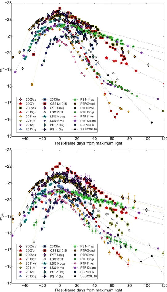
−40 −20 0 20 40 60 80 100 120 Rest-frame days from maximum light
−23 −22 −21 −20 −19 −18 −17 −16 −15 Mg 2005ap 2007bi 2008es 2010gx 2011ke 2011kf 2012il 2013dg 2013hx CSS121015 iPTF13ajg LSQ12dlf LSQ14bdq LSQ14mo PS1-10bzj PS1-10ky PS1-11ap PTF09cnd PTF09cwl PTF10hgi PTF11rks PTF12dam SCP06F6 SSS120810 −40 −20 0 20 40 60 80 100 120
Rest-frame days from maximum light −23 −22 −21 −20 −19 −18 −17 −16 −15 Mgr iz 2005ap 2007bi 2008es 2010gx 2011ke 2011kf 2012il 2013dg 2013hx CSS121015 iPTF13ajg LSQ12dlf LSQ14bdq LSQ14mo PS1-10bzj PS1-10ky PS1-11ap PTF09cnd PTF09cwl PTF10hgi PTF11rks PTF12dam SCP06F6 SSS120810
Well-observed SNe in the literature
SN1994I Ic −16.79 Filippenko et al. (1995), Richmond et al. (1996) SN1998bw IcBL‡ −16.84 Patat et al. (2001) SN1999ex Ic −16.84 Stritzinger et al. (2002) SN2002ap IcBL −16.49 Mazzali et al. (2002)
Gal-Yam, Ofek & Shemmer (2002)
SN2003jd IcBL −18.19 Valenti et al. (2008a) SN2004aw Ic −17.24 Taubenberger et al. (2006) SN2007gr Ic −16.36 Valenti et al. (2008b) SN2008D Ib −16.24 Soderberg et al. (2008),
Modjaz et al. (2009) SN2009jf Ic −17.34 Valenti et al. (2011) SN2010bh IcBL‡ −16.97 Cano et al. (2011) SN2011bm Ic −17.63 Valenti et al. (2012) SN2012bz IcBL‡ −18.82 Schulze et al. (2014) SDSS II sample from Taddia et al. (2015)
SN2005hl Ib −17.55 SN2005hm Ib −15.85 SN2006fe Ic −17.04 SN2006fo Ib −17.26 14475 IcBL −19.46 SN2006jo Ib −18.25 SN2006lc Ib −17.31 SN2006nx IcBL −19.71 SN2007ms Ic −16.95 SN2007nc Ic −16.82
‡Associated with observed gamma-ray burst
have two more objects from the Pan-STARRS1 Medium Deep Survey – PS1-10ky atz ∼0.9 (Chomiuk et al. 2011) and PS1-10bzj atz∼0.6 (Lunnan et al. 2013) – while most of the others featured in the original Quimby et al. (2011) sample that defined the SLSN Ic class. Although several of these objects are at redshifts 0.25 < z <0.3, the reddest available photometry is in the R-band, which corresponds to rest-frame B/g. SCP06F6 (z = 1.189) has HST i and z photometry (Barbary et al. 2009), which corresponds to rest-frame emission between the u- andg-bands. The final Silver object is iPTF13ajg (Vreeswijk et al. 2014), which has excellent photometric and spectroscopic coverage, but at z= 0.74 this mostly probes rest-frame UV. This means that for these objects we must rely on an estimated correc-tion to obtain bolometric light curves.
3 BOLOMETRIC LIGHT CURVES
To analyse the light curves of our SLSNe in the most ho-mogeneous way possible, we constructed two sets of light curves: rest-frameg-band magnitudes,Mg, and pseudobolo-metric light curves covering rest-frame SDSSgrizfilters. The first step was to applyK-corrections to the observed magni-tudes, to transform them to the rest-frames of our objects. These were determined as follows. We calculated synthetic photometry, using theiraf3package
calcphot, on all
avail-3 Image Reduction and Analysis Facility (IRAF) is distributed by the National Optical Astronomy Observatory, which is operated by the Association of Universities for Research in Astronomy, Inc.,
cluding a correction to the flux per unit wavelength by a fac-tor of 1 +z, and new synthetic magnitudes were calculated. TheK-correction at the epoch of a given spectrum is simply the difference between the rest-frame and observed synthetic magnitudes. These corrections were then linearly interpo-lated to the epochs with photometry. For most cases we simply correctedgobs→gRF etc., aside from the following: LSQ14bdq (robs→gRF); SN 2005ap, PTF09cnd, PTF09cwl (Robs→gRF); PS1-11ap (iobs →gRF;K-corrections taken from McCrum et al. 2014); PS1-10bzj, iPTF13ajg (iobs →
gRF); PS1-10ky (zobs→gRF); SCP06F6 (iobs, zobs→gRF). For the objects of Quimby et al. (2011), sometimes only one spectrum was available – in this case we also used the spec-tra of SN 2010gx from Pastorello et al. (2010) (a spectro-scopically typical event, with good temporal coverage), after artificially placing them at the desired redshift. Magnitudes were also corrected for Milky Way extinction according to the dust maps of Schlafly & Finkbeiner (2011), though host reddening was assumed to be negligible.
For the Gold sample, the bolometric light curve was then calculated using this rest-frame photometry from the gto z filters. For LSQ14mo, thez-band was estimated us-ing the colours of SN 2013dg, to which it has a very similar light curve in thegri-bands, while thez-band magnitudes for PS1-11ap and LSQ14bdq were taken from PTF12dam, as in McCrum et al. (2014). Most objects have good cov-erage before/around peak in one filter only. In these cases, the colours were assumed to be constant, with values from the first epoch that had multi-colour photometry available. This is a reasonable assumption, as the colours show lit-tle evolution until 1-2 weeks after maximum light (Inserra et al. 2013). A spectral energy distribution (SED) was then constructed by converting these magnitudes into flux at the effective wavelength of each filter. For all objects, the flux was set to zero blue-wards of theg-band and red-wards of z. The luminosity,Lgriz, was then calculated by integrating this SED over wavelength, and correcting for distance to the SN assuming a cosmologyH0= 72 km s−1, ΩM = 0.27, and ΩΛ= 0.73. This follows the procedure of Inserra et al. (2013). We express this in terms of pseudobolometric mag-nitude, using: Mgriz≡ −2.5 log10 Lgriz 3.055×1035 , (1)
based on the standard definition of bolometric luminos-ity. Our complete set ofg-band and pseudobolometric light curves are shown in Fig. 1.
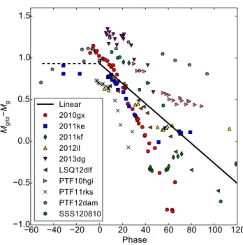
However, a different process was needed to derive the Mlight curves of the Silver objects. It was possible to find the average bolometric correction,Mgriz−Mg, as a function of time (we definet= 0 as the epoch of maximum luminos-ity), for the Gold sample, and apply this correction to our other objects. This correction is shown in Fig. 2. Unfortu-nately, there is significant scatter, but it is clear that the bolometric correction becomes more negative as a function of time. This is expected; as the SNe cool, bluer wavelengths
under cooperative agreement with the National Science Founda-tion.
−60 −40 −20 0 20 40 60 80 100 120 Phase −1.0 −0.5 0.0 0.5 1.0 1.5 Mgr iz − Mg Linear 2010gx 2011ke 2011kf 2012il 2013dg LSQ12dlf PTF10hgi PTF11rks PTF12dam SSS120810
Figure 2.Estimating the time-dependent bolometric correction for a typical SLSN. Our best fit is Mgriz−Mg= 0.90−0.012t fort >0, though the gradient can vary from this by a factor∼2 for individual objects. Uncertainty in they-intercept term has no effect on our analysis.
fade faster at late times. We fit only points where t > 0, assuming a constant correction before this. Our best fit is Mgriz−Mg= 0.90−0.012tfort >0 andMgriz−Mg= 0.90 fort <0. The uncertainty in this correction is∼0.5 magni-tudes by 50d after peak, hence at late phases the M light curves of Silver objects may become unreliable. However, note that only two Silver objects have data at this phase: PTF09cnd and PTF09cwl. Both of these objects closely re-semble PTF12dam in rest-frameg (but were not classified as being 2007bi-like), and this resemblance is preserved in the pseudobolometric light curves. Hence we feel justified in including these objects in our sample.
4 LIGHT CURVE TIMESCALES
4.1 Measurements
Having constructed our pseudobolometric light curves, we proceeded to measure the rates at which these supernovae brighten to their maximum luminosity, and subsequently de-cline. We define:
• τrise (the rise timescale): the time (t < 0) relative to maximum light (Lmax) at whichLgriz=Lmax/e
• τdec(the decline timescale): the time (t >0) relative to maximum light (Lmax) at whichLgriz=Lmax/e.
We make our measurements by fitting the light curves with low-order polynomials. Order four polynomials were found to give a good fit to all of our light curves for epochs t . 50 d. The fits were used to make a new estimate of the date when the pseudobolometric luminosity peaks. This tends to be later than the peak in g-band, as one would expect since the ejecta cool over time. We define the new
−20 0 20 40 60 80
Rest-frame days from maximum light 1042 1043 Lgr iz ³ er g s − 1 ´ Fit order = 4 Lmax/e 2010gx
Figure 3.Interpolating the light curve of SN 2010gx. The times at which the dashed line intersects the polynomial fit give the exponential rise and decline times.
peak, and then measure the quantities described above by interpolating the light curves with the polynomial fits. The method is demonstrated in Fig. 3. In some cases, the rise time had to be estimated by extrapolation using our poly-nomials. We consider this to be reliable for most objects, where we extrapolate only by a few days, but the rise time is poorly constrained for SNe 2007bi, 2005ap, and PS1-10ky. For slowly declining objects, the fourth order fit to the peak was not always a good fit at late epochs; for these objects, we made one fit tot . 50 d to estimate the peak and the rise time, as for the rest of our sample, and then measured the decline time by fitting another polynomial to only the post-maximum data points (fourth order and linear fits gave similar results). Our measurements are given in Table 3. The rise time of SSS120810 could not be constrained from the available data.
4.2 Correlation
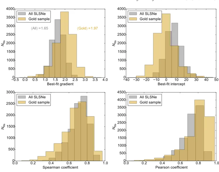
We plot the rise times vs decline times for our sample in Fig. 4. The best-fit lines to our Gold and complete samples are calculated as follows: we represent each data point by a two-dimensional Gaussian, with a mean given by our mea-sured values ofτriseandτdec, and standard deviations by the error bars. A Monte-Carlo method is then employed. A point is drawn at random from each probability distribution de-fined by these Gaussians, and we use standardPython rou-tines to calculate a straight-line fit, as well as Spearman and Pearson correlation coefficients, for the resulting rise-decline relation. This is repeated 10000 times. As can be seen in Fig. 5, the data are clearly correlated with high significance: Spearman’s rank correlation coefficient is 0.77±0.10 for the entire SLSN sample (0.75±0.11 for Gold sample only). Pear-son’s test gives 0.81±0.15 (0.84±0.14). The best-fit straight line to the data isτdec= (1.65±0.33)τrise+ (7.38±7.79) for the full sample, andτdec= (1.96±0.46)τrise+(−0.10±10.19) for the Gold objects. Although the formal best fit is different for the full sample compared to the Gold SLSNe only, the entire population is clearly consistent with a straight-line, and the two fits agree within the errors. It is no surprise
0 10 20 30 40 50 Rise timescale, τrise (days)
0 20 40 60 80 D ec lin e tim es ca le , τdec ( da ys ) τdec=τrise 94I 98bw 99ex 02ap 03jd 04aw 07gr 08D 09jf 10bh 11bm 12bz 2007bi 2008es 2010gx 2011ke 2011kf 2012il 2013dg 2013hx LSQ12dlf LSQ14mo LSQ14bdq PTF10hgi PTF11rks PTF12dam CSS121015 PS1-11ap 2005ap SCP06F6 PTF09cnd PTF09cwl PS1-10ky PS1-10bzj iPTF13ajg SN Ibc SN Ic-BL Taddia+ 2015 Ibc T15 Ic template
Figure 4.Rise vs decline timescales for SLSNe and normal stripped-envelope supernovae. The rise and decline times are clearly correlated, and in a similar way for both samples. The dashed black line gives the best linear fit to the entire SLSN sample (y= 1.65x+ 7.38), and the solid black line to the Gold sample only (y= 1.96x−0.10). The T14 Ic light curve was constructed by integrating thegriztemplates for SDSS SNe Ic from Taddia et al. (2015).
that the gradient is greater than unity, as the light curves of other SN types (both Type Ia and core-collapse) rise to maximum more quickly than they decline. We also measure rise and decline timescales for the SNe Ibc in Table 2. They obey a similar correlation as for SLSNe, but with shorter timescales than their more luminous cousins.
4.3 Models: overview
To interpret our correlation, we use the synthetic light curve code described by Inserra et al. (2013). This code al-lows us to model the luminosity from a homologously ex-panding spherical ejecta with constant opacity and a cen-trally located power source, Lin(t). The light curve equa-tion, re-derived following the original Arnett (1982) paper
but adapted for arbitraryLin, is
LSN(t) =e−(t/τm)2 Z t 0 2Lin(t0) t 0 τme (t0/τm)2dt 0 τm, (2)
where τm is the diffusion timescale (formally, the geomet-ric mean of the expansion and diffusion timescales; Arnett 1982).
In the most basic case (for a fixed form of the power in-put term,Lin, e.g. an exponentially declining term for heat-ing by radioactive decay, or a central engine with a power-law decline), our model takes three parameters: a diffusion timescale, a power input timescale (which we callτin), and an overall energy scale (which affects the luminosity of the light curve, but not the shape). In general, the diffusion timescale is a function of ejecta mass, opacity and
−0.5 0.0 0.5 1.0 1.5 2.0 2.5 3.0 3.5 4.0 Best-fLt graGLent 0 500 1000 1500 2000 2500 3000 3500 4000 NfLt s ⟨All⟩ 1.65 ⟨GolG⟩ 1.97 All 6L61e GolG samSle 0.0 0.2 0.4 0.6 0.8 1.0 3earson coeffLcLent 0 500 1000 1500 2000 2500 3000 3500 4000 4500 NfLt s All 6L61e GolG saPSle 0.0 0.2 0.4 0.6 0.8 1.0 6Searman coeffLcLent 0 500 1000 1500 2000 2500 3000 NfLt s All 6L61e GolG samSle −40 −30 −20 −10 0 10 20 30 40 50 Best-fLt LnterceSt 0 500 1000 1500 2000 2500 3000 3500 4000 NfLt s All SLS1e GolG samSle
Figure 5.Fit parameters for the rise-decline timescale correlation.
sion velocity: τm= 2κMej βcv 1/2 , (3)
where κ is the opacity, Mej is the ejected mass, β ≈13.8 (for a wide range of plausible density profiles) is an inte-gration constant,c is the speed of light and v is a scaling velocity for homologous expansion (Arnett 1980, 1982). For a given opacity and velocity, the diffusion timescale thus al-lows us to derive the mass. Other authors have taken the observed rise times of SNe as an estimate of τm (most re-cently Wheeler, Johnson & Clocchiatti 2014). This is a rea-sonable approximation for56Ni-powered light curves, where the decay time is well known, and is closely matched to the typical diffusion times (a coincidence that results in the high peak luminosities in Type Ia SNe). It is not surprising that the normal-luminosity hydrogen-poor sample shown in Fig. 4 obey a tight rise-decline correlation: the power input time is the same for all these56Ni-powered SNe, and hence the diversity in both rise and decline times is driven by only one parameter: the diffusion time. The fact that the SLSNe obey such a similar correlation suggests that the diffusion time may also drive the correlation in these objects.
However, for SLSNe the power input time,τin, is un-known, and may span a wide range of values. Ifτin is very different fromτm, it can have a large influence on the ob-served rise time, which is no longer a reliable proxy to τm. A better method here is to use the light curve width: we estimate that the diffusion time through the ejecta is τm∼(τrise+τdec)/2. This is explored in detail for the fol-lowing models, and will be important when we later attempt to estimate masses, in section 9.
4.4 Models:56Ni and generalised exponential
models
As a first step towards investigating the SLSN parame-ter space, we generated an array of models with a hypo-thetical exponentially decaying power source (i.e., with the same functional form as56Ni decay, but for a variable life-time). While this power source is not motivated by any pro-posed physical model, it aids in understanding the relevant timescales, by virtue of being the simplest possible scenario. This model takes only two parameters: the diffusion time (τm) and the input time (τin), with Lin = L0exp(−t/τin) (L0 is arbitrary). We varied the diffusion time between 10
0 10 20 30 40 50 Rise timescale, τrise (days)
0 20 40 60 80 D ec lin e tim es ca le , τdec ( da ys ) 56
Ni →
56Co →
56Fe
P(t)
∝
e
−t/τinτ
in=9d
τ
in=20d
τ
in=50d
SLSN Ic, Gold, 2005ap-like SLSN Ic, Gold, 2007bi-like SLSN Ic,Silver SLSN II SN Ibc SN Ic-BL Taddia+ 2015 Ibc Taddia+ 2015 Ic template 0 15 30 45 60 75 90 105 120 D iff us io n tim es ca le , τm ( da ys )
Figure 6.The observed rise and decline timescales of our sample overlaid on a grid of diffusion models (Arnett 1982), with a central heating term that decays exponentially with time. Input times of 10-20 d are needed to reproduce the SLSN correlation, which is then driven by variation in the diffusion timescale, as shown by the colour-bar.56Ni/56Co models are also shown (grey curve). This roughly matches the normal-luminosity SNe Ibc, although there is a slight offset, which depends on the efficiency of gamma-ray trapping (our model uses the trapping formalism of Arnett (1982), with a velocity of 10000 km s−1).
and 120 days, in steps of 10 days. A subset of these models are shown on Fig. 6. We see that, if SLSNe are powered by some universal, exponentially declining process, such a pro-cess must have a lifetime of∼10-20 days (the smaller points shown are spaced by 1 d in τin). However, if the timescale for power input is variable, SLSNe in the top right can have longer timescales (shown by the red curve and larger points, with τin= 50 d). Most importantly, this figure shows that for this simple model, the correlation in rise and decline timescales is driven byτm, as seen in the colour scale.
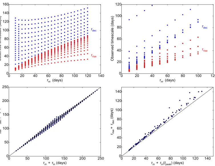
Figure 7 shows the relationship between diffusion time and measured rise/decline times for a full grid of mod-els, with τm,τin= 10-120 d, in steps of 10 days. Clearly, there is no straightforward way to deduce the diffusion time directly from either the rise or the decline. However, we find a strong correlation when the quantities are
com-bined:τrise+τdec≈τm+τin. This holds over the full range inτmand τin. Hence if we know the timescale of our expo-nential power source, we can accurately recover the diffusion time by measuring the rise and decline timescales. Measure-ment of the ejected mass through light curve fitting has been applied for many years to SNe Ibc. Since the input timescale is known for56Ni-powered SNe, the light curve width is typ-ically a measurement of the diffusion time (e.g. Arnett 1982; Drout et al. 2011; Valenti et al. 2008a). For SLSNe, most of the best-fitting exponential models haveτin∼τm. Therefore, from our relation between the 4 important timescales, an es-timate of the diffusion time is given byτm≈(τrise+τdec)/2. Figure 6 also shows the expected rise-decline curve for models powered by 56Ni-decay. In this case, the only im-portant variable is the diffusion time (56Ni mass sets the overall luminosity, but not the light curve width). We see
0 20 40 60 80 100 120 140 τm (days) 0 20 40 60 80 100 120 140 160
Observed timescale (days)
τdec τrise 0 50 100 150 200 250 τm+τin (days) 0 50 100 150 200 250 τrise + τdec ( da ys )
Figure 7. The relationships between various timescales in the simple exponential model. While neither the rise nor decline timescale is a good tracer of the diffusion time (top), the light curve width is determined by the sum of the power input and dif-fusion times, such thatτmcan be deduced from observedτriseand
τdecfor a givenτin (bottom).
that this model does predict the correlation exhibited by SNe Ibc, which must be controlled by the diffusion time as mentioned in the previous subsection. Although some of fast rising and fast decaying SLSNe Ic lie close to this56Ni decay curve, that power source has already been ruled out for these. As discussed in Chomiuk et al. (2011), Quimby et al. (2011) and Pastorello et al. (2010), the peak luminos-ity means that the56Ni mass would have to be greater than or similar to the total ejecta mass. Such expanding balls of 56
Ni are unphysical and ruled out by the observed spectra.
4.5 Models: magnetar
In one of the most popular models, SLSNe are powered by a central engine which re-shocks the ejecta after it has ex-panded to large radius, thus overcoming adiabatic losses. In the magnetar spin-down model, the energy source is the ro-tational energy of a millisecond pulsar, which is tapped via a strong magnetic field. It is generally assumed to radiate with
0 20 40 60 80 100 120 τm (days) 0 20 40 60 80 100 120
Observed timescale (days)
τrise τdec 0 20 40 60 80 100 120 140 τm+τin(tpeak) (days) 0 20 40 60 80 100 120 140 τrise + τdec ( da ys )
Figure 9.Same as Fig. 7, but for our magnetar model grid. The models shown have diffusion times of 10-100 d (steps of 10 d), B ={1,3,5,7,9} ×1014G, and P ={1,3,5,7,9}ms. Only models with peak luminosity greater than 3×1043erg s−1are plotted. the functional form of a magnetic dipole (Kasen & Bildsten 2010): Lmagnetar(t) = Ep τp 1 (1 +t/τp)2 erg s −1 , (4)
whereEp(the rotational energy,InsΩ2/2) andτpare deter-mined by the spin period,P, and magnetic field,B, of the magnetar. The energy input timescale for magnetar spin-down is given byτp= 4.75B14−2P
2
msd, whereB14is the mag-netic field in units of 1014Gauss andPms is the initial spin period in milliseconds. The shortest possible rotation period (corresponding to the largest energy reservoir) isP ∼1 ms; any shorter and centrifugal forces would lead to breakup. Galactic magnetars haveB <1015G (e.g. Davies et al. 2009, Table 3). This combination makes it difficult to achieve spin-down timescalesτp0.1 d.
We ran a grid of magnetar models, uniformly varying τm(in steps of 10 days),BandP(in unit steps of 1014G and milliseconds, respectively), which we compare to the data in Fig. 8. However, it is not obvious that we can varyB and Pindependently. The high magnetic field is likely generated
0 10 20 30 40 50 Rise timescale, τrise (days)
0 20 40 60 80 D ec lin e tim es ca le , τdec ( da ys )
Magnetar models
SLSN Ic, Gold, 2005ap-like SLSN Ic, Gold, 2007bi-like SLSN Ic,Silver SLSN II SN Ibc SN Ic-BL Taddia+ 2015 Ibc Taddia+ 2015 Ic template 10 20 30 40 50 60 70 80 90 100 D iff us io n tim es ca le , τm ( da ys ) 0 10 20 30 40 50 0 20 40 60 80 100 D ec lin e tim es ca le , τdec ( da ys )
B
0 10 20 30 40 50 0 20 40 60 80 100P
1 2 3 4 5 6 7 8 9 10 B ( 10 14 G ), P ( m s)Rise timescale, τrise (days)
Figure 8.We overlay a grid of magnetar-powered diffusion models with different spin period (P), magnetic field (B) and diffusion time (τm). All are varied in uniform steps. Only models withLpeak >3×1043erg s−1 are plotted. The top panel shows how increasing the diffusion timescale,τm, traces out the correlation we see in our data, and thatτmis the parameter most strongly driving the diversity in our light curves. The lower panels show the effect of varyingP andB. The bottom left region (where normal SNe Ic reside) is difficult to reach with magnetar models, as very highBis required. SLSN lie along the lower right edge of the magnetar distribution, whereP andBare least extreme (for givenτm).
0 20 40 60 80 100 τin(tpeak) (days) 0 5 10 15 20 25 Nm od el s
Figure 10. The distribution of the power input timescales at maximum light, for the magnetar models in Fig. 9. We caution that this is for a uniform distribution inB and P, whereas we do not know what initial spins and magnetic fields magnetars are likely to form with. In particular, models withτin<10 d require high magnetic field and fast spin.
by a dynamo mechanism during core-collapse (Duncan & Thompson 1992), as a primordialB-field in the progenitor core would couple its angular momentum to the envelope, braking the core and likely precluding formation of a mil-lisecond pulsar at collapse. The simplest assumption for the dynamo mechanism is that a constant fraction of the ro-tation energy,Ep ∝P−2, is converted to magnetic energy, Emag∝B2. In this case, we would haveB∝1/P. Using this approach (with uniformly distributed P), rather than uni-formly distributedB and P, results in no significant effect on the distribution of rise and decline timescales in Fig. 8. Bearing in mind that we do not know the initial distribu-tion of spin periods (and henceB-fields), we will continue our analysis assuming that B and P are independent pa-rameters for simplicity.
Only models that are brighter than the faintest SLSN in our sample (PTF10hgi) are plotted. We produced many more models of course, but the only ones that are relevant are those producing luminosities of the same order as the SLSNe. The models shown display a correlation in rise and decline timescales similar to that observed in SLSNe, al-though a small number of models have very slow declines relative to the rise time. The colour map shows that increas-ing τm drives the models to longer rise and decline times, tracing out the observed correlation. We also investigate the effect ofB andP. TheB-field influences the rise time, but has little effect on the decline.B∼1015G is needed to reach τrise.10 d. This could explain why no SLSNe are seen with such short rise times. The corollary also holds: if we were to observe SLSNe with rise times less than about 10 days, it would preclude the magnetar model would struggle to ex-plain them. Models with longPtend to rise quickly, but this is not a necessary condition, unlike the constraint onB.
Most of our SLSNe lie below the magnetar grid, but are consistent (within the errors) with lying along the locus of points on the sharp lower-right edge of the model
distribu-tion. This locus corresponds to weakerB, andP ∼2-5 ms. If SLSNe are powered by millisecond magnetars, the less-extreme magnetic field may account for why the data pref-erentially lie at the lower edge of the model distribution. Overall, magnetar models satisfactorily reproduce the basic trend we see in the data. For a sensible range of parameters, diffusion time dominates the diversity in timescales, just as we saw previously for the simplest models with a central (exponential) power source.
Although most of the energy injection in this model takes place within a time τp, the power input timescale is not a constant, unlike in exponential models. Using the definition τin= |Lin(t)/(dL/dt)|, we find that for magne-tars, τin(t) = 1
2(τp+t), whereas for radioactive sources, τin is simply the lifetime of the nucleus. In setting the peak width, the important timescale (in addition toτm) is τin(tpeak) = 1
2(τp+tpeak). Using this definition, we recover al-most exactly the same correlation between the 4 timescales: τrise+τdec≈τm+τin(tpeak). This is shown in Fig. 9. Does this mean that we can assumeτm≈(τrise+τdec)/2 in this case also? Fig. 10 shows the distribution ofτin(tpeak) for our magnetar grid. The mean is 19 days (standard deviation: 18 d). Of all the models, 76% haveτin between 5 and 30 days at peak; however those withτin(tpeak)<10 d need both fast rotation and strong magnetic field. This corresponds to the bottom left region in Fig. 8, where we do not have any ob-served SLSNe. Therefore the relevant models have timescales mostly in the range 10-30 d, with a tail extending to many tens of days. This is good news, as the assumption that τin∼τmis thus also reasonable for magnetar models. Hence we conclude thatτm≈(τrise+τdec)/2, for a range of sensible models with central power sources.
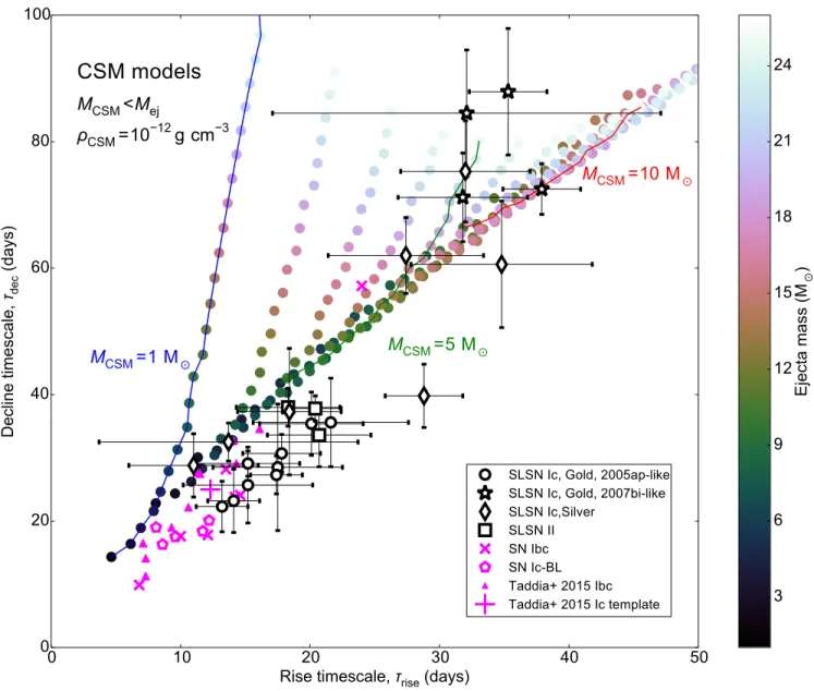
4.6 Models: CSM interaction
Alternatively, we can attempt to fit the observed correla-tions with parameterised models in which the ejecta collide with a dense CSM. This has been another popular model in-voked to explain SLSNe(Ginzburg & Balberg 2012; Cheva-lier & Irwin 2011; Moriya & Maeda 2012). As in Nicholl et al. (2014) (which followed the physical treatment of Chatzopou-los, Wheeler & Vinko 2012), we consider the limit of zero expansion velocity and luminosity input by strong external shocks. This model has many free parameters: ejected mass; CSM mass, radius and density (and density profile); explo-sion energy;56Ni mass. We ran a grid of models with fixed explosion energy (1051 erg; this mostly just affects the peak luminosity) and inner CSM radius (1012cm; the light curve is quite insensitive to this parameter), and assume no56Ni. The CSM is taken to be a spherically symmetric shell of constant density – its mass and density therefore determine its radial extent. We varied the ejected mass (Mej) in unit steps from 1-25 M, and CSM mass (MCSM) in similar steps from 1-15 M, with the additional restrictionMCSM< Mej. The CSM density was initially set toρCSM= 10−12g cm−3. The results are shown in Fig. 11. At a given MCSM, increasing Mej increases both τrise and τdec, in the same way as the diffusion time,τm, did for our magnetar models. Illustrative lines of fixedMCSMhave been marked – the ob-served rise-decline correlation is best reproduced by models withMCSM&Mej/2. This was a common feature of models presented by Nicholl et al. (2014), and in fact is probably a
0 10 20 30 40 50 Rise timescale, τrise (days)
0 20 40 60 80 D ec lin e tim es ca le , τdec ( da ys )
CSM models
M
CSM<
M
ejρ
CSM=10
−12g cm
−3M
CSM=1 M
⊙M
CSM=5 M
⊙M
CSM=10 M
⊙SLSN Ic, Gold, 2005ap-like SLSN Ic, Gold, 2007bi-like SLSN Ic,Silver SLSN II SN Ibc SN Ic-BL Taddia+ 2015 Ibc Taddia+ 2015 Ic template 3 6 9 12 15 18 21 24 E je ct a m as s (M ⊙ )
Figure 11.Same as Fig. 8, but for interaction-based models. In this case, we vary the ejected mass and CSM mass, and CSM density. We find that the shape of the rise-decline distribution is highly sensitive to the CSM density – the observed correlation is approximately recovered forρCSM= 10−12g cm−3. All of the light curve fits by Nicholl et al. (2014) (and many by Chatzopoulos et al. 2013) found
ρCSM∼10−12g cm−3. Increasing the ejecta mass moves light curves along our correlation, while increasing the CSM mass primarily affects the rise time. It can be seen that the correlation is best reproduced by the subset of models withMCSM∼Mej/2 – this was a general property of the light curve fits by Nicholl et al. (2014). Models with lower CSM mass rise too quickly for a given decline rate. If ejecta-CSM interaction does power all SLSNe, our rise-decline correlation puts tight constraints on the progenitor systems.
requirement for SLSNe powered by interaction, as the CSM mass must be an appreciable fraction of the ejecta mass to thermalise the bulk of the expansion kinetic energy.
More restrictive, but perhaps more interesting, is the effect of CSM density on our light curves. The rise-decline relation is similar to our data for ρCSM= 10−12g cm−3. In Fig. 12, we show the effect of varyingρCSMfor a few repre-sentative models. Marked on the figure is the approximate slope of the observed correlation for SLSNe. ChangingρCSM to 10−11g cm−3 or 10−13g cm−3 moves our models to re-gions of the rise-decline plot far from where our data reside. Why does this density have such a strong effect on the ratio of rise and decline times in our models? The dom-inant energy source is the forward shock from the
interac-tion, which deposits heat as it propagates through the CSM. At some point, the shock breaks out of the CSM shell, and can no longer contribute energy (a similar effect occurs with the reverse shock in the ejecta, but the forward shock turns out to be dominant in most cases); at this point our light curve usually peaks. The time taken for the forward shock to propagate through the CSM decreases with increasing den-sity (Chatzopoulos, Wheeler & Vinko 2012, equation 15). The model subsequently declines, as the stored energy dif-fuses out of the CSM, on the characteristic CSM diffusion time. This timescale increases with the CSM density, so that models with earlier peaks fade more slowly. Thus, for all other parameters fixed, there is an inverse relationship
0 20 40 60 80 100 120 Rise timescale, τrise (days)
0 20 40 60 80 100 120 140 160 D ec lin e tim es ca le , τdec ( da ys ) τdec= 2τrise ρCSM=10−11 g cm−3 ρCSM=10−12 g cm−3 ρCSM=10−13 g cm−3 Mej=5M⊙,MCSM=1M⊙ Mej=5M⊙,MCSM=5M⊙ Mej=20M⊙,MCSM=5M⊙ Mej=20M⊙,MCSM=10M⊙ −50 0 50 100 150 200 250
Rest-frame days from explosion 42.0 42.5 43.0 43.5 44.0 44.5 lo g10 ( L [e rg s − 1 ]) LSQ12dlf ρCSM=10 −11 g cm−3 ρCSM=10−12 g cm−3 ρCSM=10−13 g cm−3
Figure 12.Rise vs decline timescales for synthetic light curves powered by ejecta-CSM interaction. The relation is strongly de-pendent on the density of the CSM. Models with ρCSM ∼ 10−12g cm−3 (shown in Fig. 11) correspond best to our data. This can also be seen here in the lower panel, where we com-pare the SLSN LSQ12dlf to 3 models withMej=MCSM= 5 M, and varying CSM density. The light curves peak when the for-ward shock from the ejecta-CSM collision breaks out of the CSM, and the subsequent decline is controlled mainly by the diffusion time in the CSM. Denser CSM results in faster shock propagation (shorter rise) and slower diffusion (longer decline), giving the in-verse relationship between rise and decline times apparent in the top panel.
between rise and decline timescales as we varyρCSM, as seen in Fig. 12.
Clearly, if SLSNe are powered by interaction with a dense CSM, our observed rise-decline relationship can place narrow constraints on the range of CSM densities present. Of the 6 SLSN light curves fit with CSM models by Nicholl et al. (2014), 5 had densities in the range−12.54<log10ρCSM<
−11.74 (no convincing fit was found for the final object, SN 2011ke). It seems contrived that virtually all H-poor SLSNe would have such similar circumstellar densities, particularly when modelling indicates that a range of densities can gener-ate the observed peak magnitudes (e.g. Chatzopoulos et al. 2013, who also fit H-rich events). Three possibilities exist. The first and most obvious is that ejecta-CSM interaction is
not the power source in SLSNe Ic. Alternatively, our simple model may not be a good description of interacting SLSNe (for example, the shape of the CSM density profile may be important, and not a uniform shell). One very impor-tant weakness in this analysis is that the interaction mod-els of Chatzopoulos, Wheeler & Vinko (2012) and Nicholl et al. (2014) treat the shocks following Chevalier & Frans-son (1994), whose derivation was forMCSMMej, and it is unclear how the picture changes for massive CSM. Finally, some process in the evolution of SLSN progenitors might somehow be capable of consistently producing circumstel-lar environments within this density range. The homogene-ity in the spectral properties of SLSNe would then result from the similar physical conditions in the CSM. The last of these possibilities is intriguing, and determining this pro-cess could prove an important clue to understanding what kinds of stars produce SLSNe. However, observations of SNe known to be powered by CSM interaction (SNe IIn) show huge diversity and variation in their observed characteristics and inferred physical configurations. In any case, CSM mod-els will have to be able explain our observed correlation, if we are to continue to accept them as valid model for SLSNe.
5 GENERALISED LIGHT CURVES AND
PEAK LUMINOSITY
The correlation in rise and decline timescales, presented in the previous section, was found to be the same for SLSNe Ic and for normal-luminosity, hydrogen-poor core-collapse SNe. This suggested that the two populations have the same basic light curve shape (and we inferred that the slower evolution of SLSNe was due to longer diffusion timescales). To fur-ther investigate the relationship between SLSN and normal SN Ic light curves, we construct a generalised light curve for each type of SN. We do this simply by taking the area in magnitude-time parameter space that contains all of the light curves in each sample (SLSNe of Type II are excluded from this analysis). This is shown in Fig. 13, where we also include the SN Ibc light curve template from Taddia et al. (2015), and a number of SNe Ibc with unusually high lumi-nosity. As expected, the SLSN light curves are much brighter and broader than typical SNe Ibc. In the unscaled SN Ibc light curve, the decline rate starts to change at around 30 days after peak. This is because the ejecta are becoming op-tically thin, and the luminosity begins to track the decay of 56
Co. We do not typically see his behaviour in SLSNe, for two reasons. For most SLSNe, the decline after peak is too fast to be compatible with realistic56Ni-driven models with such a high peak luminosity, as discussed in Sect. 4.4. If they do contain some small amounts of56Co (comparable to that in SNe Ibc), this is masked by the bright luminosity source that powers the peak. The more slowly declining SLSNe (SN 2007bi-like), on the other hand, do match the56Co decay rate. If they were radioactively powered, the long rise times and broad peaks would allow them to join smoothly onto the56Co decay tail after maximum.
We find that a very simple transformation maps the SN Ic light curves onto those of the SLSNe: an increase along they-axis by 3.5 magnitudes (a multiplicative factor of≈25 in luminosity), and a broadening in time by a factor 3. The most obvious interpretation of this correspondence is that
−40 −20 0 20 40 60 Rest-frame days from maximum light −21 −20 −19 −18 −17 −16 −15 Mgr iz SLSNe Normal Ibc Normal Ibc (scaled) 1998bw 2012bz 2006nx 2011bm Taddia+ 2015 template
Figure 13. Generalised light curves for SLSNe compared with lower luminosity SNe Ic (normal and broad-lined). The blue area represents normal SNe Ic in our well-observed literature sam-ple. and those of Taddia et al. (2015). SN Ic light curves can be mapped onto the SLSNe by a 3.5 magnitude increase in bright-ness and a stretch along the time axis by a factor of 3. Some broad-lined SNe Ic lie in the magnitude gap, but tend to have narrower light curves than SLSNe. SN 2011bm (Valenti et al. 2012) shows a normal Ic spectral evolution but has a light curve width comparable to SLSNe.
the two sets of light curves are determined by the same un-derlying physics: the rapid expansion of shocked gas with small initial radius, heated by some internal power supply. The broader light curves of the SLSNe are indicative of a longer diffusion timescale (higher mass and/or lower veloc-ity) compared to the SNe Ic. The higher peak luminosity tells us that some additional energy source is heating the ejecta, compared to ∼ 0.1−1 M of 56Ni in SNe Ic (this could be, for example, a millisecond magnetar). Indeed, this is the established theory explaining the diversity within the SN Ic class, where higher ejecta mass and56Ni mass result in broader and brighter light curves, respectively.
If SLSNe Ic were powered by interaction of SN Ic ejecta with dense (and H-poor) circumstellar material, the light curve physics would be quite different: a combination of for-ward and reverse shocks in the ejecta and CSM, with a strong dependence on the various density profiles. Indeed, for the massive, optically thick CSM needed to generate super-luminous peak magnitudes, we should not actually see direct emission from the supernova ejecta until well after maximum light (Benetti et al. 2014). It would therefore be surprising to recover such a trivial transformation between normal and super-luminous Ic light curves. Circumstellar interaction can generate a range of light curve shapes (as shown in Fig. 12). For instance, the most conclusive exam-ple of a Type Ic SN interacting with H-deficient CSM is SN 2010mb (Ben-Ami et al. 2014), which had an extremely un-usual light curve shape with a plateau lasting for hundreds of days.
One interesting question is whether there is a continuum of peak luminosities between normal and super-luminous Type Ic SNe. Since the discovery and characterisation of
termine absolute magnitude distributions in the standard JohnsonB-band. Their study attempted to correct for bias and derive volume limited absolute magnitude distributions, however the targets do not all have enough data to deter-mine bolometric luminosities (Mgriz at maximum). There are some typing inaccuracies in the Richardson et al. sam-ple (e.g. 2006oz as a Ib, and 2005ap as a type II), however the normal and broad-lined Ibc population does appear to have an upper limit to their peak brightness of around−18 to−19, with the SLSNe sitting 3 magnitudes brighter.
We compare the brightness distributions of our SLSNe and other SNe in Fig. 14. The SLSNe Ic peak atMgriz=
−20.72±0.59 magnitudes, while the normal SNe Ibc tend to peak atMgriz=−17.03±0.58. We note here that Inserra & Smartt (2014) derived peak absolute magnitudes for a sample of 16 SLSNe (with a large overlap with our sam-ple) in a synthetic bandpass centred on 400 nm. They found
hM400i = −21.86±0.35. This seems to be more uniform thanMgriz, though it is worth bearing in mind that in some cases our derivedMgriz has been estimated using assumed colours, introducing additional uncertainty, whereas Inserra & Smartt (2014) had observations fully covering their syn-thetic bandpass for all of their objects at maximum light.
Selection effects and bias in our sample mean we cannot definitively say whether there is an excess of hydrogen-poor supernovae with peak absolute magnitudes brighter than Mgriz∼ −20 (i.e. SLSNe), or whether such events are the bright tail of a continuous magnitude distribution. The plot in Fig. 14 is not meant be be a representative luminosity function, as one would require accurate relative numbers in either a magnitude or volume limited survey. We know definitively that SLNSe are rare and their relative rate with respect to normal SNe Ibc is of order 1 SLSNe per 3000-10000 SNe Ibc (Quimby et al. 2013; McCrum et al. 2015). The SLSNe are obviously over-represented in our sample, relative to their rates of occurrence in nature, as we have compiled similar numbers of SLSNe and comparison SNe Ibc. To prove statistically that SLSNe comprise a separate population of events from the brightest ‘normal’ SNe Ic would require careful consideration of the selection factors in surveys such as PTF, PS1 and LSQ+PESSTO to determine unbiased relative numbers of SLSNe, SNe Ibc, and SNe Ic-BL and construct meaningful luminosity functions (e.g. as done for normal SNe in Li et al. 2011)
Nevertheless we can make some comments on the lu-minosity differences observed if we assume that the SNe Ibc we have compiled are fairly representative of the gen-eral population of such stripped envelope SNe. None of our spectroscopically normal SNe Ibc are observed to peak at Mgriz≈ −19. However, some broad-lined SNe Ic do have peak magnitudes spanning the gap between normal and super-luminous SNe. Broad-lined SNe Ic are often high56 Ni-producers, and some have been shown to be associated with observed gamma-ray bursts (GRBs) (Woosley & Bloom 2006). The large56Ni mass makes them brighter than typical SNe Ic. Fig. 13 shows two GRB-SNe, SN 1998bw (Patat et al. 2001) and SN 2012bz (Schulze et al. 2014). The brightest Ic-BL in the sample of Taddia et al. (2015) is also shown. The object, SN 2006nx, was discovered at redshiftz= 0.137, but if there was an associated GRB, it was not seen. SN 2006nx
actually has a similar peak magnitude to SLSNe, suggesting that it may in fact be a member of that class. However, its light curve is quite narrow not only compared to SLSNe, but also for such a luminous56Ni-powered SN. Its unknown spectral evolution precludes a robust answer to the question of whether it is physically related to the SLSN population.
It is interesting that some SNe Ic-BL/GRB-SNe do lie in the gap between SNe Ic and SLSNe, as some authors have suggested that SLSNe and GRBs are in fact related. Lun-nan et al. (2014) argued that the two types of explosion oc-cur in similar low-metallicity environments. Leloudas et al. (2015) also claimed that their host galaxies are similar, but also that those of SLSNe are more intensely star-forming than those of GRBs, perhaps implying more massive pro-genitors for SLSNe. Magnetar/engine-powered models have been invoked to explain both the high luminosities in SLSNe and the relativistic jets in GRB-SNe(Thompson, Chang & Quataert 2004; Metzger et al. 2011). However, the required magnetar parameters in GRB models are more extreme than for SLSNe, with spin periods∼1 ms and magnetic fields 10-100 times stronger, in order to drive a jet that punches through the stellar envelope (Bucciantini et al. 2009). Gal-Yam (2012) notes that some broad-lined SNe Ic, such as SN 2007D (Drout et al. 2011) and SN 2010ay (Sanders et al. 2012), reached peak magnitudes close to those of SLSNe, and likely required an additional energy source on top of the inferred∼1 Mof56Ni. Perhaps bright SNe Ic-BL represent events where the central engine enhances the luminosity as well as the kinetic energy of the explosion, but not to the same degree as in SLSNe, where the additional power source overwhelms the input from 56Ni decay. In this framework, there could thus be a continuum in luminosity between the various subclasses of SNe Ic, depending on the properties of the engine.
If, however, there is a significant gap in peak bright-ness, with very few objects intermediate between normal and super-luminous SNe Ic, it may be difficult to explain for circumstellar interaction models. For example, Type II su-pernovae show a broad but continuous distribution in peak magnitudes: from SNe II-P through Type II-L’s to bright Type IIn and SLSNe IIn. Some authors have argued that this hierarchy is driven by varying degrees of circumstellar interaction (Chevalier & Fransson 1994; Richardson et al. 2002; Gal-Yam 2012). A gap between SNe/SLSNe Ic could be more indicative of a threshold process – for example, only progenitors above some critical mass can form magne-tars, or undergo a particular instability (e.g. pulsational pair instability; Woosley, Blinnikov & Heger 2007). In the mag-netar model, there may also exist an observational ‘desert’ between cases where the spin-down power is sufficient to drive a stable jet (GRB), and cases where the spin-down is weaker and slower, forming a wind nebula and enhancing the late-time luminosity instead (SLSN). If the magnetar spins down very quickly but the jet does not break the stellar en-velope, there may be neither a GRB nor an enhancement in optical brightness (B. Metzger, private communication.) In summary, peak magnitude distributions of SNe from large, homogeneous samples are needed, and will provide an impor-tant constraint on the possible relationships between SLSNe and SNe Ic.
Table 3.Measured properties and derived masses SN τrise(d)a τdec(d)b v5169 (km s−1)c Mej/M Super-luminous SNe SN2007bi 32.1 84.5 11900 31.1+34.3−21.7 SN2008es∗ 18.3 38.0 – 3.7+3.0−2.1 SN2010gx 15.2 29.1 10900 4.4+3.2−2.3 SN2011ke 15.2 25.7 10200 3.3+1.9−1.5 SN2011kf 17.5 28.5 9000 3.7+2.0−1.5 SN2012il 14.1 23.2 9100 2.4+1.3−1.0 SN2013dg 17.8 30.7 14000 6.3+3.8−2.9 SN2013hx 20.7 33.6 6000 3.4+1.8−1.4 LSQ12dlf 20.1 35.4 13700 8.1+5.1−3.9 LSQ14mo 17.4 27.3 10200 3.9+1.9−1.5 LSQ14bdq† 31.8 71.2 – 20.4+18.6 −12.6 PTF10hgi 21.6 35.6 4800 3.0+1.7−1.3 PTF11rks 13.2 22.3 18100 4.4+2.5−2.0 PTF12dam 37.9 72.5 10500 27.0+19.6−14.3 CSS121015 20.4 37.8 10000‡ 6.5+4.5−3.3 SSS120810 – 30.2†† 11200 5.7+3.6 −2.1 PS1-11ap† 35.3 87.9 – 29.2+30.3 −19.6 SN2005ap† >11 28.8 – 3.0+3.3−2.1 SCP06F6† 28.8 39.8 – 9.1+3.1−2.7 PTF09cnd† 32.0 75.3 – 22.2+21.5−14.3 PTF09cwl† 34.8 60.6 – 17.5+10.8 −8.2 PS1-10ky† 13.7 32.5 – 4.1+4.0 −2.7 PS1-10bzj 18.4 37.3 13000 7.8+6.2−4.4 iPTF13ajg 27.4 62.0 9100 14.0+12.9−8.7 Other H-poor SNe
SN1994I 6.8 9.9 10100 0.5+0.2−0.2 SN1998bw 12.2 20.1 26600 5.3+2.9−2.3 SN1999ex 12.1 17.8 9300 1.6+0.7−0.6 SN2002ap 8.1 19.0 20400 2.9+2.8−1.9 SN2003jd 9.6 17.5 16400 2.3+1.5−1.2 SN2004aw 13.5 28.2 12100 4.1+3.4−2.4 SN2007gr 10.0 17.6 8400 1.2+0.8−0.6 SN2008D 14.6 24.1 8700 2.5+1.4−1.1 SN2009jf 14.2 23.8 10100 2.8+1.6−1.2 SN2010bh 8.6 16.3 35000 4.2+3.0−2.2 SN2011bm† 24.0 57.2 – 12.7+12.5−8.3 SN2012bz 11.7 18.4 23000 4.0+2.0−1.6 SN2005hl 14.3 29.1 5450‡ 2.0+1.6−1.1 SN2005hm 11.5 27.5 9470‡ 2.8+2.7−1.8 SN2006fe 11.3 27.7 5000‡ 1.5+1.5−1.0 SN2006fo 14.1 32.7 10500‡ 4.4+4.2 −2.8 14475 7.3 14.1 18700‡ 1.6+1.2 −0.9 SN2006jo 7.3 11.3 14400‡ 1.0+0.5−0.4 SN2006lc 9.3 19.0 9100‡ 1.4+1.1−0.8 SN2006nx 7.1 16.5 15400‡ 1.7+1.6−1.1 SN2007ms 16.1 34.6 11400‡ 5.6+4.9 −3.4 SN2007nc 10.6 22.2 12700‡ 2.6+2.2 −1.5 Masses derived using equation 5 withκ= 0.1 cm2g−1andτ
m= (τrise+τdec)/2. Error bars correspond to estimates with τm=
τrise(lower) andτm=τdec(upper).aCharacteristic time for SN to rise to maximum light, defined using τrise≡ t(Lpeak/e) for
t < tpeak;bcharacteristic time to fade,τdec≡t(Lpeak/e) fort >
tpeak;cVelocity from minimum of Fe IIλ5169 absorption, 20-30 d after maximum light;∗Assumesv∼6000 km s−1, based on SN 2013hx spectrum; ‡Velocity from the literature, not necessarily Fe II;†Assumesv= 10000 km s−1;††For mass estimate, we take τrise=τdec/1.6 (see Fig. 4)
−22 −21 −20 −19 −18 −17 −16 −15 Mgriz at maximum 0 2 4 6 8 Nob je ct s ⟨Full sample⟩=−20.81 SNe Ibc SNe Ic-BL
Figure 14. The distribution of magnitudes at maximum light. The scatter is quite low, with a standard deviation of only 0.50 magnitudes (0.58 if we include the two SLSNe II). The mean peak magnitude for normal SNe Ic is−17.03. A few broad-lined events have luminosity comparable to the fainter SLSNe. The data are binned in 0.5 mag intervals.
6 TWO TYPES OF SLSN IC?
For most SLSNe, the data unambiguously exclude56Ni and 56Co decay as the main power source around light curve maximum: the 56Ni-mass needed to power the peak is of the order of the total ejected mass inferred from light curve fitting, and moreover exceeds the limiting 56Ni-mass in-ferred from the late-time luminosity (e.g. Inserra et al. 2013). However, Gal-Yam (2012) proposed that the events with broader light curves, such as SN 2007bi, are radioactively powered, and likely exploded as pair-instability SNe. These would be fundamentally different from the other SLSNe, having a different explosion mechanism and power source, and would be characterised observationally by longer light curve timescales. We now look to see if we can distinguish two distinct classes in our data. In fact, Fig. 4 shows a rel-ative lack of SLSNe withτrise∼25-30 d and withτdec∼ 40-60 d. To make this clearer, we plot histograms ofτrise,τdec, and theg-band decline in magnitude 30 days after maximum light. This is a proxy for the decline timescale that is much simper to observationally measure, and particularly useful for parameterising the decline in high-redshift SLSNe, which may not have good rest-frame coverage in the redder bands. The data are shown in Fig. 15.
We apply the Dip Test of Hartigan & Hartigan (1985) to each parameter. The dip statistic,D, measures the max-imum difference between the empirical distribution and a unimodal distribution (chosen so as to minimiseD). A larger value of D indicates that the data are not well described by a unimodal probability distribution function (PDF). We test for multi-modality using a bootstrapping method. We construct 5000 random sets of length n, where n is the size of our SLSN sample (n = 19 for our full sample), drawn from a uniform PDF, and calculate D for each set. The probability p-value for the null hypothesis to be cor-rect (i.e. that the data are unimodal) is then given by p =N(DSLSNe < Dboot)/5000 (this is the fraction of
ran-5 10 15 20 25 30 35 40 45
Rise timescale (days) 0 1 2 3 4 5 6 NS LS N e SLSNe II 20 30 40 50 60 70 80 90
Decline timescale (days) 0 1 2 3 4 5 6 7 NS LS N e SLSNe Ic SLSNe II 0.0 0.5 1.0 1.5 2.0 2.5 Δg30 (mag, RF) 0 1 2 3 4 5 6 NS LS N e SLSNe Ic SLSNe II
Figure 15.Histograms showing the rise (top) and decline ( mid-dle) timescales (binned in 5 day intervals), and theg-band decline (binned in 0.25 mag intervals) in 30 days after maximum (bottom). While the distributions show some indication of bimodality by eye, applying Hartigan’s Dip Test (Hartigan & Hartigan 1985) shows that this is not statistically significant.