Empirical Comparisons of Different Statistical Models To Identify and Validate Kernel Row Number-Associated Variants from Structured Multi-parent Mapping Populations of Maize

(1)

University of Nebraska - Lincoln

DigitalCommons@University of Nebraska - Lincoln

Agronomy & Horticulture -- Faculty Publications

Agronomy and Horticulture Department

2018

Empirical Comparisons of Different Statistical Models To Identify

and Validate Kernel Row Number-Associated Variants from

Structured Multi-parent Mapping Populations of Maize

Jinliang Yang

University of Nebraska-Lincoln, [email protected]

Cheng-Ting Yeh

Iowa State University

Raghuprakash Kastoori Ramamurthy

University of Nebraska-Lincoln, [email protected]

Xinshuai Qi

University of Arizona

Rohan L. Fernando

Iowa State University

See next page for additional authors

Follow this and additional works at:

https://digitalcommons.unl.edu/agronomyfacpub

Part of the

Agricultural Science Commons

,

Agriculture Commons

,

Agronomy and Crop Sciences

Commons

,

Botany Commons

,

Horticulture Commons

,

Other Plant Sciences Commons

, and the

Plant

Biology Commons

Yang, Jinliang; Yeh, Cheng-Ting; Ramamurthy, Raghuprakash Kastoori; Qi, Xinshuai; Fernando, Rohan L.;

Dekkers, Jack C. M.; Garrick, Dorian J.; Nettleton, Dan; and Schnable, Patrick, "Empirical Comparisons of

Different Statistical Models To Identify and Validate Kernel Row Number-Associated Variants from

Structured Multi-parent Mapping Populations of Maize" (2018). Agronomy & Horticulture -- Faculty

Publications. 1143.

https://digitalcommons.unl.edu/agronomyfacpub/1143

This Article is brought to you for free and open access by the Agronomy and Horticulture Department at

DigitalCommons@University of Nebraska - Lincoln. It has been accepted for inclusion in Agronomy & Horticulture -- Faculty Publications by an authorized administrator of DigitalCommons@University of Nebraska - Lincoln.

(2)

Authors

Jinliang Yang, Cheng-Ting Yeh, Raghuprakash Kastoori Ramamurthy, Xinshuai Qi, Rohan L. Fernando,

Jack C. M. Dekkers, Dorian J. Garrick, Dan Nettleton, and Patrick Schnable

This article is available at DigitalCommons@University of Nebraska - Lincoln: https://digitalcommons.unl.edu/ agronomyfacpub/1143

(3)

MULTIPARENTAL POPULATIONS

Empirical Comparisons of Different Statistical

Models To Identify and Validate Kernel Row

Number-Associated Variants from Structured

Multi-parent Mapping Populations of Maize

Jinliang Yang,*,†_Cheng-Ting“_Eddy”_{Yeh,* Raghuprakash Kastoori Ramamurthy,}†_{Xinshuai Qi,}‡

Rohan L. Fernando,§Jack C. M. Dekkers,§Dorian J. Garrick,§Dan Nettleton,** and Patrick S. Schnable*,1

*Department of Agronomy,§Department of Animal Science and Center for Integrated Animal Genomics, **Department of Statistics, Iowa State University, Ames, IA 50011,†Department of Agronomy and Horticulture, University of Nebraska-Lincoln, Nebraska-Lincoln, NE 68583, and‡Department of Ecology and Evolutionary Biology, University of Arizona, Tucson, AZ

ORCID IDs: 0000-0002-0999-3518 (J.Y.); 0000-0002-1392-2018 (C.-T.E.Y.); 0000-0002-7804-712X (R.K.R.); 0000-0001-5821-099X (R.L.F.); 0000-0001-9169-5204 (P.S.S.)

ABSTRACT Advances in next generation sequencing technologies and statistical approaches enable genome-wide dissection of phenotypic traits via genome-genome-wide association studies (GWAS). Although multiple statistical approaches for conducting GWAS are available, the power and cross-validation rates of many approaches have been mostly tested using simulated data. Empirical comparisons of single variant (SV) and multi-variant (MV) GWAS approaches have not been conducted to test if a single approach or a combination of SV and MV is effective, through identification and cross-validation of trait-associated loci. In this study, kernel row number (KRN) data were collected from a set of 6,230 entries derived from the Nested Association Mapping (NAM) population and related populations. Three different types of GWAS analyses were performed: 1) single-variant (SV), 2) stepwise regression (STR) and 3) a Bayesian-based multi-variant (BMV) model. Using SV, STR, and BMV models, 257, 300, and 442 KRN-associated variants (KAVs) were identified in the initial GWAS analyses. Of these, 231 KAVs were subjected to genetic validation using three unrelated populations that were not included in the initial GWAS. Genetic validation results suggest that the three GWAS approaches are complementary. Interestingly, KAVs in low recombination regions were more likely to exhibit associations in independent populations than KAVs in recombinationally active regions, probably as a consequence of linkage disequilibrium. The KAVs identified in this study have the potential to enhance our understanding of the genetic basis of ear development.

KEYWORDS GWAS KRN maize Bayesian Multiparent Advanced Generation Inter-Cross (MAGIC) multiparental populations MPP

Following the adoption of genome wide association studies (GWAS) (Kleinet al.2005),2,000 loci have been identiﬁed as being statistically associated with human disease and other quantitative traits (Visscher

et al.2012). Using GWAS approaches, hundreds of loci associated with traits have been identiﬁed in crops including maize (Brownet al.2011; Tianet al.2011; Leiboffet al.2015), rice (Huanget al.2010), sorghum (Morriset al.2013) and barley (Cockramet al.2010), and in non-crop models such asArabidopsis(Atwellet al.2010; Meijónet al.2014).

There are multiple statistical models for conducting GWAS, in-cluding both single-variant (SV) and multi-variant (MV) models. SV analysis compares the phenotypic distributions of alternative genotypes at each polymorphic site independently. They can be conducted without correction for population structure or with correction using techniques such as genomic control (Devlin and Roeder 1999) or principal com-ponent analysis (Priceet al.2006). More recently, genetic relatedness among individuals can be accounted using a kinship matrix in mixed linear models (Yuet al.2006). Although SV analysis is often used in Copyright © 2018 Yanget al.

doi:https://doi.org/10.1534/g3.118.200636

Manuscript received August 2, 2018; accepted for publication August 31, 2018; published Early Online September 13, 2018.

This is an open-access article distributed under the terms of the Creative Commons Attribution 4.0 International License (http://creativecommons.org/ licenses/by/4.0/), which permits unrestricted use, distribution, and reproduction in any medium, provided the original work is properly cited.

1_{Corresponding author: Patrick S. Schnable ([email protected])}

(4)

published literature, it has a number of inherent limitations, such as not being able to distinguish among the contributions of closely linked loci (Yanget al.2012). Sometimes SV analysis overcorrects for the genomic inflation of the test statistics caused by genetic structure because cova-riates identified via population structure analysis can be associated with causal loci (Yanget al.2011). In comparison, MV models have already been demonstrated to be superior in classical linkage analyses, where for example, composite interval mapping outperforms simple interval mapping (Zeng 1993). MV models can explicitly account for large-effect loci and estimate the large-effects of multiple loci simultaneously. It has been suggested that the power of GWAS may be improved by conditioning on major-effect QTL (Kanget al.2010). One challenge to using MV models, however, is the substantial computational burden associated with analyzing a large number of polymorphic sites. As a partial solution, stepwise regression, which selects markers based on forward inclusion and backward elimination, has been proposed (Seguraet al.2012). As an alternative to stepwise regression, multi-variant Bayesian models that were initially developed for genomic pre-diction, by simultaneouslyfitting all genotyped loci across the genome (Meuwissenet al.2001), have been used for GWAS (Fanet al.2011; Habieret al.2011). These Bayesian-based approachesfit hierarchical models that allow the effects of many loci to shrink toward zero. An empirical comparison of the above models is necessary to investigate their relative advantages in dissecting the genetic architecture of target traits (either individually or in combination).

Many models for conducting GWAS have been compared using simulated data (Galeslootet al.2014). Although such studies can pro-vide insight, they suffer from the limitation that simulated data do not necessarily reﬂect all characteristics of real data because some charac-teristics of empirical data may be unknown to the simulator. Hence, comparisons based on empirical data are complementary to those based on simulated data. Other than studies that compared different versions of mixed linear model approaches (Stichet al.2008), to our knowledge there are no published reports that compare results gener-ated from empirical data analyzed using single-variant (SV), stepwise regression (STR) and Bayesian-based multi-variant (BMV) models for GWAS. In this study, our objective is to compare the effectiveness and/or complementarity of different GWAS (SV, STR, and BMV) models using a single empirical data set. Our second objective is to assess the degree to which ourﬁndings from different GWAS models would support other independent empirical data sets.

We perform our initial GWAS analyses on four populations (de-scribed in Material and Methods) related to the nested association mapping (NAM) population, which combines the strengths of histor-ical recombination events across a broad base of genetic diversity and recombination events that arise following experimental crosses (Yu et al.2008). Rather than studying diversity panels often featured in GWAS, we consider multi-parent mapping populations to take advan-tage of the statistical power of QTL mapping and the gene-level reso-lution of association mapping.

We study the kernel row number (KRN) phenotype, which is both a component of yield and a model trait for genetic studies in maize (Hallaueret al.2010). KRN is highly heritable and a polygenic trait (Liuet al.2015a,b) that exhibits little variation in response to environ-ment (Luet al.2011). In addition, KRN is easily scored as an integer, and this scoring can be conducted after completion of the busy polli-nation season. We collected new KRN data and downloaded previously published KRN data (Brownet al.2011).

Collectively, the three GWAS models identiﬁed 988 unique KRN-associated variants (KAVs), 231 of which were subjected to genetic validation tests using three unrelated populations that were not included

in the initial GWAS. Approximately 60% of the validated KAVs were identiﬁed by only one of the three approaches.

MATERIALS AND METHODS

KRN phenotyping for initial GWAS populations

KRN phenotypes were collected from four related populations: 1) the nested association mapping (NAM, N = 4,699) population which was composed of 25 recombinant inbred line (RIL) subpopulations (Yuet al. 2008), plus RILs of intermated B73 and Mo17 (IBM, N = 325) (Leeet al. 2002), 2) a subset of the RILs that were backcrossed to the inbred line B73 (B73 x RILs, N = 692 BC1 lines), 3) a subset of the RILs that were backcrossed to the inbred line Mo17 (Mo17 x RILs, N = 289 BC1 lines) and 4) a partial diallel created from the 26 NAM founders and Mo17 (N = 225 F1 hybrids). Because reciprocal crosses were not con-sidered and some of the crosses were not successful, the diallel popu-lation was both partial and incomplete (225/351 = 64%).

During the years 2008-2011, NAM RIL populations were sequen-tially planted in Ames, IA (summer season) and in Molokai, HI (winter season), such that only a fraction of the full set of RILs were grown in a given environment. For each NAM RIL,ﬁve plants were grown within each row. KRN data were collected from the mature ears. In addition, we obtained KRN data from eight trials for NAM RILs from a previous study (Brownet al.2011). The Brown et al.(2011) data set is eight times larger than ours. We obtained

final phenotypic values byfitting a mixed linear model withfixed effects for entries and random effects for trials. Phenotypic density distributions in this study were estimated and plotted using R with default smoothing parameters.

During the summer of 2011, the B73 x RILs, Mo17 x RILs, and the diallel populations (GWAS populations 2-4) were planted in Ames, IA in 12-plant rows. The B73 x RILs and Mo17x RILs were planted with two replications, and the diallel population was planted with three replications. For each replication, KRN data were collected from three mature ears. The obtained KRN phenotypic data were analyzed using a mixed linear model, where genotype wasfitted as afixed factor and replication wasfitted as a random factor.

KRN phenotyping for subsequent validation populations

Elite maize inbred lines, extreme KRN USDA accessions, and lines obtained from Iowa long ear synthetic (BSLE) population were used for genetic validation of KAVs identiﬁed through GWAS. A total of 220 elite inbred lines, commercial lines that had formerly been subject to IP (Intellectual Property) protection via the plant variety protection act, were obtained from the USDA Plant Introduction (PI) Station in Ames, IA (http://www.ars.usda.gov/main/site_main.htm?modecode=36-25-12-00). During year 2011, these accessions were planted in three rep-lications and observed for KRN phenotypes. About 7,000 of the maize accessions have been phenotyped for the KRN trait in the database of USDA PI Station. We selected the 225 accessions with the largest KRN values, the 208 accessions with the smallest KRN values, and 173 random accessions to serve as the second genetic validation pop-ulation. Empirical KRN phenotypes were obtained from our previously published replicated ﬁeld experiment (Yanget al.2015). Because of the genetic heterogeneity of the accessions, up to 12 random seeds were germinated and pooled together for each accession for DNA isolation. The BSLE population was the product of a long-term selection proj-ect conducted to divergently selproj-ect long and short ears from a single founder population (Hallaueret al.2004). Parental lines (N = 10/12) of BSLE and bulked seeds from cycle 0 (C0), cycle 30 short ear (C30 SE)

(5)

and cycle 30 long ear (C30 LE) were obtained from Arnel Hallauer as our third validation population.

Genomic variant processing

A set of 6.2 million genic variants (SNPs and small InDels) was identified via analysis of RNA-seq data fromfive tissues (shoot apical meristem, ear, tassel, shoot and root) on 26 NAM founder lines and Mo17 (Linet al. 2017). Another two sets of genomic variants generated from the maize HapMap project (Bukowski et al.2015) were extracted from the Panzea database (https://www.panzea.org). These three sets of var-iants were merged using the consensus mode of PLINK (Purcell et al.2007). The merged variants were furtherfiltered by discarding variants with a call rate of,0.4 across entries. We furtherfiltered variants using a minor allele frequency (MAF) cutoff of,0.1 to exclude minor SNPs only present in fewer thanfive non-B73 par-ents. The finalized set consists of 12,966,279 genomic variants on NAM founders, which were used for imputation or projection onto the four related GWAS populations.

Imputation of genotypes was performed as described below. NAM RILs had been directly genotyped using genotyping-by-sequencing (GBS) technology (Elshireet al.2011). We obtained the GBS data from the Panzea database (https://www.panzea.org). Based on the GBS data and the known pedigrees, the13 million variants discovered in the NAM founders were imputed onto NAM RILs using a python script (https://github.com/yangjl/zmSNPtools) as previously described (Yu et al.2008). Because the B73xRIL, Mo17xRIL and partial diallel pop-ulations were composed of pairs of known haplotypes, their geno-types were directly projected from their parents using the above python script.

Association variants thinning

Because progeny of bi-parental crosses comprised much of the initial GWAS population, the strong linkage of genetic variants violated the assumption of independence needed to determine statistical-based thresholds. Therefore, a variant thinning procedure was developed to select the most significant variants, and to avoid concentration of selected variants in certain regions. For variants located in the 28 QTL intervals from the joint QTL analysis and their 1-Mb flanking re-gions, the top 10 most significant variants were selected. For variants located in other regions, significant variants were determined follow-ing the arbitrary thresholds:2log10ðPÞ.20 for the SV model, pos-terior model frequency (MF) . 0.02 for the BMV model and an inclusionPvalue,0.05 for the stepwise regression. These significant variants were clustered as groups if none of their pair-wise physical distances exceeded 10-Mb. From these clustered groups, no more than 10 most significant variants were selected.

Amplicon sequencing for validation of KAVs

Amplicon sequencing assays were designed for 140/231 (61%) KAVs. A total of 1,102 DNA samples from elite inbred lines (N = 208), extreme KRN lines from the USDA germplasm collection (N = 606) and individuals from the Iowa Long Ear Synthetic (BSLE, N = 288) were individually genotyped, by sequencing all multiplexed ampli-cons from all 1,102 samples in one HiSeq2000 lane. Informative variants, deﬁned as those which were successfully genotyped, were polymorphic, and had a call rate of.0.4 and a MAF.0.05 were used for genetic validation.

Statistical Analysis: Joint QTL analysisJoint linkage analysis was performed on NAM and IBM RILs using their corresponding genetic

maps. A two-step composite interval mapping (CIM) (Zeng 1993) method was employed using a suite of programs within QTL cartog-rapher (Silva Lda et al.2012). First, an automatic forward stepwise regression procedure was used to sequentially test all SNP markers; the most significant marker (inclusion threshold = 0.05) was kept after each iteration. This procedure was repeated until no SNP met the in-clusion threshold. In the second step, linkage analyses were conducted at 1-Mb intervals along the chromosome treating previously selected SNPs (other than those within the 1-Mb interval under analysis) as co-variates. A significance threshold was determined by conducting 1,000 permutations and QTL confidence intervals were defined using a 1.5-LOD drop from QTL peak (Lander and Botstein 1989).

To account for documented stratiﬁcation effects, the statistical model includedﬁxed effects for population and subpopulation for all three GWAS models described below.

Single-variant (SV) GWAS model Additionalﬁxed effects were

ﬁtted in the model to control for effects of QTL on other chromosomes, while all variants on a single chromosome were scanned, resulting in the following model 1 for thekth variant:

Yl ¼ukþ X4 i¼1 aikPilþ X26 j¼1 bjkSjlþ X m2ChðkÞ ckmQmlþdkVARklþekl (1) where Yl is the adjusted KRN phenotypic value for linelfrom the mixed linear model analysis;ukis an intercept parameter;Pilis 1 if linelis of GWAS populationiand is 0 otherwise, andaikis the effect of theith population in the model for variantk;Sjlis 1 if linelis from subpopulation jand 0 otherwise,bjkis the effect of subpopulation jin the model for variantk;Qmlindicates the linelgenotype of the mth QTL detected by the joint linkage analyses,ckmis the effect of the mth QTL in the model for variantk,ChðkÞis the set of QTL detected by the joint linkage analysis that are located on chromosomes other than the chromosome of variantk;VARklindicates the genotype of thekth variant in linel,dkis the effect of thekth variant; andeklis an error term. This SV model 1 was implemented using SNPTEST v2.3.0 (Marchini and Howie 2010).

Stepwise regression (STR) GWAS modelIn the stepwise regression test, population and subpopulation effects werefittedfirst asfixed effects, and then markers were added in a stepwise manner. For each marker,R2 was calculated as the proportion of sums of squares after thefixed effects. We employed the STR method that was implemented in GenSel v4.1 (Habieret al.2011) with the option of“StepWise”. We used the following three options to control the STR model, 1) inputMaxRs-quared (default 0.8), inputMaxMarkers (300) and alphaValue (default 0.05).

Bayesian-based multi-variant (BMV) GWAS modelA Bayesian-based MV model was constructed using the“BayesC”option of GenSel v4.1 (Habieret al.2011). This model differs from the SV model in that it estimates the effects of all variants simultaneously rather than testing them one-at-a-time. The effects of the variants wereﬁtted as random effects. The following mixed model was used.

Yl ¼uþ X4 i¼1 aiPilþ X26 j¼1 bjSjlþ X 13M k ckVARklþel (2)

whereVARklindicates the genotype of thekth variant in linelandckis the effect of thekth variant; other terms in the model are as described in the SV model 1 except that neither theu,ai;orbjparameters nor theelerror terms are speciﬁc to thekth variant in the BMV model 2.

(6)

We trained the BMV model using a two-step procedure. In theﬁrst step, we ran 1,000 iterations with 100 burn in of MCMC simulation using default priors,i.e., genetic variance (genVariance = 1) and residual var-iance (resVarvar-iance = 1). In the 2nd_{step, we replaced the priors using the} posteriors obtained from step 1 and ran a longer chain of simulations (chainLength = 41,000 and burnIn = 1,000).

Data Availability

File S1 contains phenotypic data for the GWAS populations. File S2 contains the KAVs identified using the three GWAS models. File S3 contains genotypes of KAVs for the three validation populations. File S4 contains the KRN phenotypic data for the validation populations. In the table,“Internal_id”could be used as the identifier to match genotypic data. File S5 contains the genetic validation results. Stars indicate SNPs that were consistently associated with KRN in initial GWAS, and in at least one of the validation populations. All the supplementary files have been uploaded to Figshare (10.6084/m9.

ﬁgshare.6902144). R code for the analyses is available in the public

GitHub repository (https://github.com/yangjl/KRN-GWAS). Supple-mental material available at Figshare: 10.6084/m9.ﬁgshare.6902144.

RESULTS

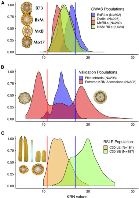
KRN Phenotype in GWAS and Validation Populations We collected KRN phenotypic data from 6,230 entries within four related GWAS populations grown at two locations over four years (see Materials and Methods). Best linear unbiased estimators (BLUE) of the KRN phenotype were calculated for each of the 6,230 entries in the four GWAS populations (File S1). In this combined analysis, KRN pheno-typic values ranged from 9.1 to 23.6, with a mean of 14.9 rows, whereas the B73 inbred had an above average KRN phenotype of 17.1 rows. Density plots of the four GWAS populations exhibited the expected bell-shaped distributions (Figure 1A).

We also collected KRN data from three unrelated populations for subsequent validation purpose. The three populations consist of elite inbred lines that expired from US plant variety protection (Nelsonet al.2008),

Figure 1 Phenotypic distributions of the KRN trait in GWAS and validation populations. (A) Density plots of the four GWAS populations. Embedded picture shows the typical KRN counts for B73, B73xMo17 (BxM), Mo17xB73 (MxB) and Mo17 lines. (B) Density plots of two validation populations, elite inbred lines and treme KRN accessions. Embedded pictures shows ex-amples of an extreme low KRN accession and an extreme high KRN accession. (C) Density plots of cycle 30 long ear (C30 LE) and cycle 30 short ear (C30 SE) in the BSLE population. Embedded pictures indicate the ear length and KRN variation after 30 generations of selection. Blue and red dashed lines indicate the mean KRN values of B73 (KRN = 17.1) and Mo17 (KRN = 10.8).

(7)

extreme KRN accessions from USDA germplasm database, and a long term selection population—Iowa long ear synthetic (BSLE). The elite lines have KRN that are less extreme and less variable than the NAM lines (Figure 1B). Thisfits with our understanding of breeder practices; they do not select for high KRN phenotypes. The USDA Plant Intro-duction station maintains a large collection of maize germplasm. The KRN phenotypes in this population are extreme, ranging from an average of 13-30 rows in the high KRN pool to 6-12 rows in the low KRN pool according to data obtained from a replicatedfield trial (Figure 1B) (Yanget al.2015). The BSLE population had been subjected to 30 generations of divergent selection for long ears (LE) and short ears (SE) (Hallaueret al.2010). During selection, KRN exhibited a nega-tively correlated response to ear length (r¼ 20:6;Pearson’s correla-tion testPvalue ,0:05),i.e., longer and shorter ears had smaller and larger KRN trait values, respectively (Figure 1C). The parental lines and bulked seeds from cycle 0 (C0), cycle 30 long ear (C30 LE) and cycle 30 short ear (C30 SE) served as our third genetic validation population. Identification of KAVs With different statistical models using GWAS populations

In each GWAS model, population and subpopulation were included as

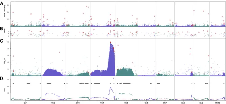
fixed effects to account for inherent structure in the 6,230 entries included in the GWAS. First, a SV model (Manolio 2010) was used to scan the13M variants one-by-one using QTL detected in the joint analysis as covariates. The linear mixed model with genetic relationship matrix was not used here because the four initial GWAS populations are NAM and NAM related multi-parent mapping populations. Using an arbitrary cutoff of2log10ðPÞ.20;this approach identified linked clusters of variants (Figure 2C), most of which were located within the 28 QTL intervals that had been identified by the joint QTL analysis (Figure 2D). To diminish the over-representation of certain regions by significant variants, a binning (bin size = 100-kb) procedure was used that resulted in the identification of 257 KAVs, which in combination accounted for 51% of the KRN variation.

Second, in an attempt to improve mapping resolution, a STR approach was used, which resulted in identiﬁcation of 300 KAVs representing 296 100-kb bins (Figure 2B). In combination, these vari-ants accounted for 78% of phenotypic variation.

Third, a BMV model (Habieret al.2011) was used to estimate effects of all13M variants simultaneously. After applying the variant thin-ning procedure and cutoffs described in Materials and Methods, a set of 442 variants representing 343 100-kb bins, which together accounted for 74% of the phenotypic variation, was identiﬁed (Figure 2A). Most promisingly, this model identiﬁed smaller chromosomal intervals than the SV model.

Comparison of KAVs identified by three GWAS Models In combination, the three GWAS models identified 764 100-kb bins (File S2), each of which contained one or more significant variants. Encour-agingly, among these 764 bins, 66 (containing 169 variants) were detected by at least two models. Only one of these bins was detected by all three GWAS models. That bin (chr4:229.0-Mb) overlaps the most significant QTL peak detected in the joint QTL study. To estimate an upper bound for cross-validation rate for each approach and to determine whether the KAVs that were detected by more than one approach are more reliable, a set of 231 KAVs was selected for genetic validation. This set of KAVs included the 169 variants in the 66 bins detected by at least two approaches and 62 of the most significant one or two variants selected from 20 bins that had only been detected by one approach (approach-specific variants). Hence, in total 231 KAVs from a total of 126 bins (66 + 20·3) were selected for genetic validation.

Collectively, the 231 selected KAVs explained 64% of phenotypic variation in the initial GWAS population byﬁtting these KAVs simul-taneously using an additive model (i.e., narrow-sense heritability h2_{64%) . Individually, most of the KAVs (83%, 192/231) explained} less than 5% of the phenotypic variation, but 17% (39/231) of the KAVs individually accounted between 5–10% of phenotypic variation.

Figure 2 Stacked plots of GWAS and QTL results. From upper to lower panels are results from the Bayesian-based multi-variant (A) stepwise regression (B) and single variant(C) models for GWAS and the joint QTL mapping result (D). The red dashed line in the QTL plot indicates the 1,000 permutation threshold and black lines show the QTL conﬁdence intervals. Red squares in panel (A), triangles in panel (B) and circles in panel (C) indicate the kernel row number associated variants selected for further genetic validation.

(8)

Note that a causal variant might be represented by multiple selected KAVs. The B73 variant-types were alleles for higher KRN for nearly three-quarters (73%, 168/231) of these KAVs, consistent with the high KRN value of the B73 genotype. Consistent with our previous study (Liet al.2012), KAVs are substantially enriched for variants located within genes or within 5-kb upstream of genes (2.0-fold change, Chi-squarePvalue,0.01) and enriched in variants discovered from the RNA-seq data (1.ninefold change, Chi-squarePvalue,0.01) relative to the13M variants used for GWAS.

Genetic validation of KAVs using three unrelated populations

To distinguish true positive association signals from potentially false pos-itive associations, three previously described genetic validation populations that are unrelated to the GWAS populations and to each other were genotyped at the KAVs (genotype data are provided in File S3 and S4).

To control for population structure in the elite inbred lines, a set of SNPs that had previously been used to genotype a subset (N = 91) of these lines was obtained (Nelsonet al.2008). Weﬁtted a mixed linear model to estimate theﬁxed effects of KAVs. In the model, we included random effects for lines. These random effects were assumed to be correlated according to a kinship matrix calculated from the genome-wide SNPs (Nelsonet al.2008). Using this approach, 22/70 (31%) of the informative KAVs could be genetically validated in the set of 91 elite inbreds with an FDR,0.05. Because the elite inbreds are not closely related to the GWAS populations, it is unlikely that uncontrolled pop-ulation structure could yield false-positive validation assays for KAVs derived from the GWAS populations. Hence, we also conducted a naive analysis using the entire set of elite inbreds (N = 209) without control-ling for population structure. In this analysis, 33/70 (47%) of the KAVs, which included all of the 22 KAVs discussed above, could be validated.

Because extreme KRN accessions were maintained via random pollination within accessions, individual accessions are both hetero-geneous and heterozygous. We therefore genotyped pools of DNA extracted from up to 12 plants per accession. A model ﬁtted to the estimated allele frequencies was used to test the hypothesis that alleles for higher KRN have higher frequencies in the high KRN pools than in low KRN pools. Among the 56/131 (43%) informative variants, 14/56 (25%) could be validated.

Of the 51 informative KAVs in the BSLE population, 7/51 (14%) showed signiﬁcant differences in allele frequency between C30 LE and C30 SE populations. To rule out the possibilities of genetic drift or stochastic sampling error, we conducted simulation to mimic the selection procedure. After simulation, one validated KAV did not pass the cutoff (FDR,0.05) and was removed. Hence, even after accounting for drift and stochastic sampling errors, 6/51 (12%) KAVs were deemed to have been under divergent selection. We applied the simulation to the negative control variants, and they were indeed negative. Collectively, these loci account for 40% of the total between-population variance for KRN trait. Variants that are segregating in BSLE but not in GWAS populations or that were simply not detected as being KAVs in the GWAS populations may explain the remaining phenotypic variation between C30 LE and C30 SE.

Summary of the genetic validation results

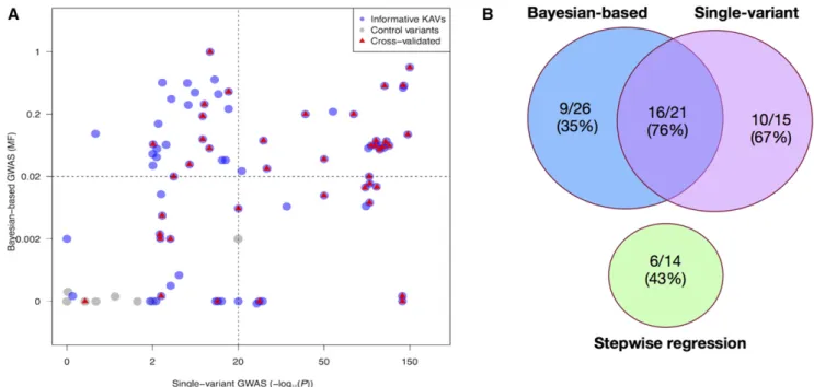
In summary, 40/77 (52%) of informative KAVs exhibited associations with the KRN trait in at least one of the genetic validation populations (File S5). The genetic validation results from the three GWAS models are illustrated in Figure 3. Considering all KAVs detected by each approach, the validation rates were 61% (20/33) for the single-variant approach, 43% (6/14) for the stepwise regression approach and 45% Figure 3 Genetic validation results of selected kernel row number associated variants (KAVs). (A) Transformed P values using single variant (SV) model and posterior model frequencies using Bayesian-based multi-variant (BMV) model were extracted and plotted for the 77 informative KAVs identiﬁed by at least one of the three GWAS models. KAVs detected only by the SV model are plotted in the lower right quadrant, KAVs detected only by the stepwise regression model are plotted as non-gray dots in the lower left quadrant, the KAVs detected only by the BMV model are plotted in the upper left quadrant, KAVs detected by both the SV and BMV models are plotted in the upper right quadrant and control variants are plotted as gray dots in the lower left quadrant. Validated KAVs are marked in red. A control variant is a genomic variant that is randomly chosen from a set of SNPs that were not associated with KRN in the initial GWAS. (B) Venn diagram of the validation results.

(9)

(14/31) for the Bayesian-based approach (Figure 3B). Validation rates were 67% (10/15) for KAVs detected only by the SV model, 43% (6/14) for those detected only by STR model, 35% (9/26) for KAVs detected only by the BMV model, 73% (16/22) for KAVs detected by both SV and BMV models, and 11% (1/9) for control variants that are randomly chosen from a set of SNPs that were not associated with KRN in the initial GWAS (Figure 3A). Although both the STR and BMV models had lower validation rates than the SV model, these results demonstrate that each of the three models identiﬁed validated KAVs that were not identiﬁed by other approaches. Thus, the three GWAS models are complementary.

We also obtained genotyping data for 34 KAVs reported in an earlier GWAS (Brownet al. 2011). Using the statistical analyses described above, 26% (9/34) of these KAVs could be validated in at least one of the three unrelated populations.

The amount of genetic recombination per Mb in maize varies substantially across the genome (Fuet al.2002). To investigate whether the probability of genetic validation varies based on the amount of recombination per Mb, the 111 tested KAVs (77 from this study and 34 from Brownet al.(2011)) were projected onto the NAM genetic map (Buckleret al.2009) using our previously published method (Liuet al. 2009). Recombination rates (cM/Mb) were estimated for every 10 cM window. KAVs were classiﬁed as being located in regions recombina-tionally “cold”(,1 cM/Mb) or “hot” (. 1 cM/Mb) chromosomal regions. KAVs located in recombinational cold zones were 3.5·more likely to be genetically validated than those in recombinational hot zones (Chi-squarePvalue,0.03).

DISCUSSION

GWAS is typically associated with high rates of false discovery (Visscher et al.2012). In human studies, a second cohort is often used to genet-ically validate the most significant SNPs discovered in thefirst cohort, thereby cost effectively reducing the number of false discoveries (Sladek et al.2007). To our knowledge, no large sets of genetic variants iden-tified via GWAS as being associated with a trait of interest has been subjected to this type of genetic validation in maize. Here, we report on such a set of genetic variants that were consistently detected as being associated with KRN in both the initial GWAS and the validation populations, each of which therefore has the potential to enhance our understanding of ear development in maize.

Each GWAS model has its own strengths and weaknesses. Results from our study indicate that the three GWAS models complement each other through initial association studies and cross-validation of KAVs. In this study, genetic validation strategies that exploit the extensive genetic resources of maize were used to estimate maximum rates of cross-validation. This was accomplished by testing whether KAVs identiﬁed via the GWAS also exhibit associations with the KRN trait in independent populations. We tested not only KAVs in or near genes that had previously been associated with the KRN trait via functional analyses, but also KAVs that were not located in or near genes with prior evidence of affecting the KRN trait. There are multiple reasons for a KAV that would not be genetically cross-validated. These include biological differences in the genetic control of the KRN trait among populations and Type II errors in the validation analyses.

Overall, at least 52% (40/77) of KAVs were cross-validated in at least one of three unrelated populations. Because KRN is mainly controlled by additive effect loci (Brownet al.2011; Luet al.2010), traits controlled by different modes of inheritance may yield different validation results. Because the four GWAS populations were all derived from 27 founder lines, they differ from a diversity panel with respect to the genetic

base. While diversity panels exploit LD from a broader genetic base, multi-parent mapping populations are usually derived from few foun-ders (narrow genetic base), which could also contribute to different validation results. Therefore, it may not be possible to generalize our results from these structured multi-parent mapping populations to other types of populations such as diversity panels. Further, GWAS conducted in plants often have access to immortalized genotypes and replicated observations, which provides the opportunity to better control for stochastic factors, such as environmental effects, that could affect the rate of false discovery as compared to GWAS con-ducted on humans or some other species.

Although the SV model had a somewhat higher genetic validation rate than the other two models (possibly at least partly because of analytic similarities between the SV model and the genetic validation experi-ments), each GWAS model identiﬁed validated KAVs that were not detected by the others. By deﬁnition, this means that the three GWAS models are complementary. Therefore, the use of multiple approaches or the development of a statistical model that combines their advantages, promises to enhance the power of GWAS.

The genetic validation rate of KAVs identiﬁed in this experiment (40/77 = 52%) is higher than KAVs identiﬁed in an earlier KRN GWAS study (9/34 = 26%) (Brownet al.2011). The improved power of our study (which made use of data from Brownet al.(2011), as well as additional data generated as part of the current study) could be due to the use of three complementary GWAS models for identifying KAVs, the inclusion of more genotypes, more phenotypic data and/or higher marker density.

KAVs located in chromosomal regions with low rates of re-combination (cM/Mb) were 3.5 times more likely to be genetically validated than those in chromosomal regions with high rates of recombination per physical distance. This is probably a consequence of the relationship between recombination and LD (Kimet al.2007). Speciﬁcally, a KAV that is not causative but that is only linked to the causative variant is more likely to exhibit an association with the KRN trait in an independent population if it is located in a large LD block as compared to a KAV that is in a region with low LD, as a consequence of higher rates of recombination separating a marker from the functional polymorphism across different genetic backgrounds.

In conclusion, this study identiﬁed hundreds of KAVs that in combination explained 64% of phenotypic variation for KRN in lines that sample60% of the genetic diversity of maize (Liuet al.2003). Over 50% of KAVs that were tested could be genetically validated. In-depth analyses of KAV-linked genes will enable us to better un-derstand the molecular and developmental processes that control var-iation in the KRN trait and may eventually be useful in breaking the negative correlation between KRN and ear length, thereby increasing grain yields.

ACKNOWLEDGMENTS

We gratefully acknowledge Dr. Arnel Hallauer, Dr. Kendall Lamkey and Mr. Paul White of Iowa State University and Dr. Candice Gardner of the USDA’s North Central Regional Plant Introduction Station (NCRPIS) for sharing genetic stocks, Drs. Sanzhen Liu (currently Kan-sas State University) and Ed Allen (Monsanto) for useful discussions, Dr. Wei Wu (currently LGC Genomics), Dr. Haiying Jiang (currently Shenyang Agricultural University), Dr. Li Li (currently China Agricul-tural University), Ms. Uyen Pham and Ms. Talissa Sari for technical support, and Ms. Lisa Coffey for the generation and maintenance of genetic stocks. We also thank anonymous reviewers for their suggestions.

(10)

LITERATURE CITED

Atwell, S., Y. S. Huang, B. J. Vilhjálmsson, G. Willems, M. Hortonet al., 2010 Genome-wide association study of 107 phenotypes in Arabidopsis thaliana inbred lines. Nature 465: 627–631.https://doi.org/10.1038/ nature08800

Brown, P. J., N. Upadyayula, G. S. Mahone, F. Tian, P. J. Bradburyet al., 2011 Distinct Genetic Architectures for Male and Female Inﬂorescence Traits of Maize. PLoS Genet. 7: e1002383.https://doi.org/10.1371/journal. pgen.1002383

Buckler, E. S., J. B. Holland, P. J. Bradbury, C. B. Acharya, P. J. Brownet al., 2009 The genetic architecture of maizeﬂowering time. Science 325: 714–718.https://doi.org/10.1126/science.1174276

Bukowski, R., X. Guo, Y. Lu, C. Zou, B. Heet al., 2015 Construction of the third generation zea mays haplotype map. Gigascience 7: 1–12.https:// doi.org/10.1093/gigascience/gix134

Cockram, J., J. White, D. L. Zuluaga, D. Smith, J. Comadranet al., 2010 Genome-wide association mapping to candidate polymorphism resolution in the unsequenced barley genome. Proc. Natl. Acad. Sci. USA 107: 21611–21616.https://doi.org/10.1073/pnas.1010179107

Devlin, B., and K. Roeder, 1999 Genomic Control for Association Studies. Biometrics 55: 997–1004.https://doi.org/10.1111/j.0006-341X.1999.00997.x Elshire, R. J., J. C. Glaubitz, Q. Sun, J. A. Poland, K. Kawamotoet al.,

2011 A robust, simple genotyping-by-sequencing (gbs) approach for high diversity species. PLoS One 6: e19379.https://doi.org/10.1371/ journal.pone.0019379

Fan, B., S. K. Onteru, Z. Q. Du, D. J. Garrick, K. J. Stalderet al.,

2011 Genome-wide association study identiﬁes loci for body composi-tion and structural soundness traits in pigs. PLoS One 6: e14726.https:// doi.org/10.1371/journal.pone.0014726

Fu, H., Z. Zheng, and H. K. Dooner, 2002 Recombination rates between adjacent genic and retrotransposon regions in maize vary by 2 orders of magnitude. Proc. Natl. Acad. Sci. USA 99: 1082–1087.https://doi.org/ 10.1073/pnas.022635499

Galesloot, T. E., K. Van Steen, L. A. Kiemeney, L. L. Janss, and S. H. Vermeulen, 2014 A comparison of multivariate genome-wide association methods. PLoS One 9: e95923.https://doi.org/10.1371/journal. pone.0095923

Habier, D., R. L. Fernando, K. Kizilkaya, and D. J. Garrick, 2011 Extension of the bayesian alphabet for genomic selection. BMC Bioinformatics 12: 186.https://doi.org/10.1186/1471-2105-12-186

Hallauer, A. R., M. J. Carena, and J. d. Miranda Filho, 2010 Quantitative genetics in maize breeding, Vol. 6. Springer Science & Business Media, Berlin, Germany.

Hallauer, A. R., A. J. Ross, and M. Lee, 2004 Long-term Divergent Selection for Ear Length in Maize 24.

Huang, X., X. Wei, T. Sang, Q. Zhao, Q. Fenget al., 2010 Genome-wide association studies of 14 agronomic traits in rice landraces. Nat. Genet. 42: 961–967.https://doi.org/10.1038/ng.695

Kang, H. M., J. H. Sul, S. K. Service, N. Zaitlen, S.-Y. Konget al., 2010 Variance component model to account for sample structure in genome-wide associa-tion studies. Nat. Genet. 42: 348–354.https://doi.org/10.1038/ng.548 Kim, S., V. Plagnol, T. T. Hu, C. Toomajian, R. M. Clarket al.,

2007 Recombination and linkage disequilibrium in Arabidopsis thali-ana. Nat. Genet. 39: 1151–1155.https://doi.org/10.1038/ng2115 Klein, R. J., C. Zeiss, E. Y. Chew, J.-Y. Tsai, R. S. Sackleret al.,

2005 Complement factor H polymorphism in age-related macular de-generation. Science 308: 385–389.https://doi.org/10.1126/

science.1109557

Lander, E. S., and S. Botstein, 1989 Mapping mendelian factors underlying quantitative traits using RFLP linkage maps. Genetics 121: 185. Lee, M., N. Sharopova, W. D. Beavis, D. Grant, M. Kattet al.,

2002 Expanding the genetic map of maize with the intermated B73 x Mo17 (IBM) population. Plant Mol. Biol. 48: 453–461.https://doi.org/ 10.1023/A:1014893521186

Leiboff, S., X. Li, H.-C. Hu, N. Todt, J. Yanget al., 2015 Genetic control of morphometric diversity in the maize shoot apical meristem. Nat. Com-mun. 6: 8974.https://doi.org/10.1038/ncomms9974

Li, X., C. Zhu, C.-T. Yeh, W. Wu, E. M. Takacset al., 2012 Genic and nongenic contributions to natural variation of quantitative traits in maize. Genome Res. 22: 2436–2444.https://doi.org/10.1101/gr.140277.112 Lin, H.-y., Q. Liu, X. Li, J. Yang, S. Liuet al., 2017 Substantial contribution

of genetic variation in the expression of transcription factors to pheno-typic variation revealed by erd-gwas. Genome Biol. 18: 192.https://doi. org/10.1186/s13059-017-1328-6

Liu, K., M. Goodman, S. Muse, J. S. Smith, E. Buckleret al., 2003 Genetic structure and diversity among maize inbred lines as inferred from DNA microsatellites. Genetics 165: 2117–2128.

Liu, L., Y. Du, D. Huo, M. Wang, X. Shenet al., 2015a Genetic architecture of maize kernel row number and whole genome prediction. Theor. Appl. Genet. 128: 2243–2254.https://doi.org/10.1007/s00122-015-2581-2 Liu, L., Y. Du, X. Shen, M. Li, W. Sunet al., 2015b Krn4 controls

quanti-tative variation in maize kernel row number. PLoS Genet. 11: e1005670. https://doi.org/10.1371/journal.pgen.1005670

Liu, S., C. T. Yeh, T. Ji, K. Ying, H. Wuet al., 2009 Mu transposon insertion sites and meiotic recombination events co-localize with epigenetic marks for open chromatin across the maize genome. PLoS Genet. 5: e1000733. https://doi.org/10.1371/journal.pgen.1000733

Lu, M., C. X. Xie, X. H. Li, Z. F. Hao, M. S. Liet al., 2011 Mapping of quantitative trait loci for kernel row number in maize across seven en-vironments. Mol. Breed. 28: 143–152. https://doi.org/10.1007/s11032-010-9468-3

Manolio, T., 2010 Genomewide association studies and assessment of the risk of disease. N. Engl. J. Med. 363: 166–176.https://doi.org/10.1056/ NEJMra0905980

Marchini, J., and B. Howie, 2010 Genotype imputation for genome-wide association studies. Nat. Rev. Genet. 11: 499–511.https://doi.org/10.1038/ nrg2796

Meijón, M., S. B. Satbhai, T. Tsuchimatsu, and W. Busch, 2014 Genome-wide association study using cellular traits identiﬁes a new regulator of root development in Arabidopsis. Nat. Genet. 46: 77–81.https://doi.org/ 10.1038/ng.2824

Meuwissen, T. H., B. J. Hayes, and M. E. Goddard, 2001 Prediction of total genetic value using genome-wide dense marker maps. Genetics 157: 1819–1829.

Morris, G. P., P. Ramu, S. P. Deshpande, C. T. Hash, and T. Shah,et al., 2013 Population genomic and genome-wide association studies of agroclimatic traits in sorghum. Proceedings of the National Academy of Sciences of the United States of America 110: 453–8.

Nelson, P. T., N. D. Coles, J. B. Holland, D. M. Bubeck, S. Smithet al., 2008 Molecular characterization of maize inbreds with expired us plant variety protection. Crop Sci. 48: 1673–1685.https://doi.org/10.2135/ cropsci2008.02.0092

Price, A. L., N. J. Patterson, R. M. Plenge, M. E. Weinblatt, N. Shadicket al., 2006 Principal components analysis corrects for stratiﬁcation in ge-nome-wide association studies. Nat. Genet. 38: 904–909.https://doi.org/ 10.1038/ng1847

Purcell, S., B. Neale, K. Todd-Brown, L. Thomas, M. R. Ferreiraet al., 2007 PLINK: a tool set for whole-genome association and population-based linkage analyses. Am. J. Hum. Genet. 81: 559–575.https://doi.org/ 10.1086/519795

Segura, V., B. J. Vilhjálmsson, A. Platt, A. Korte, U. Serenet al., 2012 An efﬁcient multi-locus mixed-model approach for genome-wide association studies in structured populations. Nat. Genet. 44: 825–830.https://doi. org/10.1038/ng.2314

Silva Lda, C., S. Wang, and Z. B. Zeng, 2012 Composite interval mapping and multiple interval mapping: Procedures and guidelines for using windows QTL cartographer. Methods Mol. Biol. 871: 75–119.https://doi. org/10.1007/978-1-61779-785-9_6

Sladek, R., G. Rocheleau, J. Rung, C. Dina, L. Shenet al., 2007 A genome-wide association study identiﬁes novel risk loci for type 2 diabetes. Nature 445: 881–885.https://doi.org/10.1038/nature05616

Stich, B., J. Möhring, H.-P. Piepho, M. Heckenberger, E. S. Buckleret al., 2008 Comparison of mixed-model approaches for association mapping. Genetics 178: 1745–1754.https://doi.org/10.1534/genetics.107.079707

(11)

Tian, F., P. J. Bradbury, P. J. Brown, H. Hung, Q. Sunet al., 2011 Genome-wide association study of leaf architecture in the maize nested association mapping population. Nat. Genet. 43: 159–162.https://doi.org/10.1038/ng.746 Visscher, P. M., M. A. Brown, M. I. McCarthy, and J. Yang, 2012 Five Years

of GWAS Discovery. Am. J. Hum. Genet. 90: 7–24.https://doi.org/ 10.1016/j.ajhg.2011.11.029

Yang, J., T. Ferreira, A. P. Morris, S. E. Medland, P. F. Maddenet al., 2012 Conditional and joint multiple-SNP analysis of GWAS summary statistics identiﬁes additional variants inﬂuencing complex traits. Nat. Genet. 44: 369–375.https://doi.org/10.1038/ng.2213

Yang, J., H. Jiang, C.-T. Yeh, J. Yu, J. A. Jeddelohet al., 2015 Extreme-phenotype genome-wide association study (xp-gwas): a method for identifying trait-associated variants by sequencing pools of individuals selected from a diversity panel. Plant J. 84: 587–596.https://doi.org/ 10.1111/tpj.13029

Yang, J., M. N. Weedon, S. Purcell, G. Lettre, K. Estradaet al., 2011 Genomic inﬂation factors under polygenic inheritance. Eur. J. Hum. Genet. 19: 807–812.https://doi.org/10.1038/ejhg.2011.39 Yu, J., J. B. Holland, M. D. McMullen, and E. S. Buckler, 2008 Genetic

design and statistical power of nested association mapping in maize. Genetics 178: 539–551.https://doi.org/10.1534/genetics.107.074245 Yu, J., G. Pressoir, W. H. Briggs, I. Vroh Bi, M. Yamasakiet al., 2006 A

uniﬁed mixed-model method for association mapping that accounts for multiple levels of relatedness. Nat. Genet. 38: 203–208.https://doi.org/ 10.1038/ng1702

Zeng, Z. B., 1993 Theoretical basis for separation of multiple linked gene effects in mapping quantitative trait loci. Proc. Natl. Acad. Sci. USA 90: 10972–10976.https://doi.org/10.1073/pnas.90.23.10972

Communicating editor: J. Holland