Implicit Bayesian Inference Using Option Prices

(1)

ISSN 1440-771X

AUSTRALIA

DEPARTMENT OF ECONOMETRICS

AND BUSINESS STATISTICS

Implicit Bayesian Inference Using Option Prices

Gael M Martin, Catherine S Forbes and Vance L Martin

(2)

Implicit Bayesian Inference Using Option Prices

Gael M. Martina_{, Catherine S. Forbes}a _{and Vance L. Martin}b∗

a. Department of Econometrics and Business Statistics, PO Box 11E

Monash University, Vic., 3800, Australia; Email: Gael.Martin@BusEco.monash.edu.au. Phone: 61 3 9905 1189; Fax: 61 3 9905 5474.

b. Department of Economics, University of Melbourne.

First Draft, July, 2000

(Monash University Working Paper 5/2000) This Version, February, 2003

Abstract

A Bayesian approach to option pricing is presented, in which posterior inference about the underlying returns process is conducted implicitly via observed option prices. A range of models allowing for conditional leptokurtosis, skewness and time-varying volatility in returns are considered, with posterior parameter distributions and model probabilities backed out from the option prices. Models are ranked according to several criteria, including out-of-sampleÞt, predictive and hedging performance. The method-ology accommodates heteroscedasticity and autocorrelation in the option pricing errors, as well as regime shifts across contract groups. The method is applied to intraday op-tion price data on the S&P500 stock index for 1995. Whilst the results provide support for models which accommodate leptokurtosis, no one model dominates according to all criteria considered.

Keywords: Bayesian Option Pricing; Leptokurtosis; Skewness; GARCH Option Pricing; Option Price Prediction; Hedging Errors.

JEL Classifications: C11, C16, G13.

∗_{This research has been supported by an Australian Research Council Large Grant. The authors would} like to thank an Associate Editor and two referees for very constructive and insightful comments on an earlier draft of the paper. All remaining errors are the responsibility of the authors.

(3)

1 Introduction

An option is a contingent claim whose theoretical price is dependent upon the process as-sumed for returns on the underlying asset on which the option is written. Observed market option prices thus contain information on this process which is potentially diﬀerent from and more complete than, information contained in an historical time series on returns; see, for example, Pastorello, Renault and Touzi (2000). In this paper, a methodology is pre-sented for conducting implicit inference about a range of models for the underlying returns process, using option price data. The methodology is based on the Bayesian paradigm and involves the production of both posterior densities for the parameters of the alternative mod-els and posterior model probabilities. The modmod-els considered allow for both time-varying conditional volatility, using the Generalized Autoregressive Conditional Heteroscedasticity (GARCH) framework of Engle (1982) and Bollerslev (1986), and leptokurtosis and skew-ness in the conditional distribution of returns, using the frameworks of Lye and Martin (1993, 1994) and Fernandez and Steel (1998). The generalized local risk-neutral valuation method of Duan (1999) is used as the basis for deÞning the pertinent risk-neutral process in the estimation of all models which assume a nonnormal conditional distribution. An important feature of the proposed framework is that it nests the option pricing model of Black and Scholes (1973), in which returns are assumed to be normally distributed with constant volatility.

To assess the out-of-sample performance of the diﬀerent parametric models, Þt and predictive densities are produced. The hedging performance of the diﬀerent models is also gauged via the construction of posterior densities for the hedging errors. The posterior densities for the model parameters and the posterior model probabilities are based on the prices of option contracts on the S&P500 stock index recorded during theÞrst 239 trading days of 1995. The out-of-sampleÞt, predictive and hedging error assessments are based on data recorded during the week immediately succeeding the end of the estimation period.1

Most of the existing statistical work on option prices is based on either the classical par-adigm or on a simple application of statisticalÞt. Engle and Mustafa (1992), Sabbatini and Linton (1998) and Heston and Nandi (2000) minimize the sum of squared deviations between observed and theoretical option prices to estimate the parameters of GARCH processes. Dumas, Fleming and Whaley (1998) adopt a similar approach using deterministic volatility models, whilst Jackwerth and Rubenstein (2001) use measures of Þt to infer a variety of deterministic and stochastic volatility models. Bates (2000), Chernov and Ghysels (2000),

(4)

and Pan (2002) use more formal classical methods to produce implicit estimates of the para-meters of stochastic volatility models, based on the assumption of conditional normality for the returns process. In Lim et al (1998), Bollerslev and Mikkelsen (1999), Duan (1999) and Hafner and Herwartz (2001),GARCH models are augmented with nonnormal conditional errors and the implications of such models for option pricing investigated, again within a classical inferential framework. In Corrado and Su (1997), Dutta and Babbel (2002) and Lim, Martin and Martin (2002a), option prices are used to conduct classical implicit estima-tion of returns models which accommodate skewness and leptokurtosis, with a time-varying volatility component also speciÞed in the case of Lim, Martin and Martin (2002a). SigniÞ -cant option-implied skewness and excess kurtosis is found in all cases, with the link between these features and implied volatility smiles highlighted in Lim, Martin and Martin (2002a). Backus, Foresis, Li and Wu (1997) also focus on the connection between volatility smiles and departures from lognormality in the underlying spot price process. Lim, Martin and Martin (2002b) extend this type of modelling approach to the less usual case of volatility frowns, linking this feature to the presence of thin-tailed underlying returns processes.

Some Bayesian analyses have been performed. Boyle and Ananthanarayanan (1977) and Korolyi (1993) conduct Bayesian inference in an option pricing framework using returns data, with attention restricted to the Black-Scholes (BS) model. Bauwens and Lubrano (2002) also use returns data to conduct Bayesian inference, but allow for deviations from theBS assumptions. In line with the present paper, Jacquier and Jarrow (2000) conduct Bayesian inference using observed option prices. Unlike our approach, however, in which the option price data is used to estimate and rank a full set of parametric returns models, Jacquier and Jarrow focus on theBS model, catering for the misspeciÞcation of that model nonparametrically. We also use a richer speciÞcation for the option pricing errors than do the latter authors. Jones (2000), Eraker (2001), Forbes, Martin and Wright (2002) and Polson and Stroud (2002) use option prices to estimate stochastic volatility models for returns, applying Bayesian inferential methods. In all cases, however, the assumption of conditional normality is maintained.

The paper is organized as follows. Section 2 discusses the application of the Bayesian statistical paradigm to option pricing. Alternative option price models that allow for time-varying volatility and nonnormality in the conditional distribution of returns are formulated in Section 3, along with the appropriate risk-neutral adjustments. In Section 4, implicit Bayesian inference based on option price data on the S&P500 index is illustrated. Posterior quantities are reported, together with summary measures of theÞt, predictive and hedging

(5)

distributions for the diﬀerent models. The empirical results provide evidence which favours a fat-tailed model, with both point and interval estimates indicating that the option prices have factored in the assumption of a returns distribution with excess kurtosis. The model which allows for excess kurtosis has the largest posterior probability and the best out-of-sample performance according to most criteria considered. There is evidence of a small amount of negative skewness being factored into the option prices, more than would be warranted by consideration of the skewness properties of returns on the index during the relevant time period. However, little posterior weight is assigned to the model which departs from normality only in the sense of being skewed. TheGARCH models are also assigned little posterior weight in comparison with the constant volatility models, although within the GARCH class there is a clear hierarchy, with the models which allow for conditional nonnormality performing better overall than the model which adopts a normal conditional distribution for returns. The hedging results suggest that the hedging errors for all models are insubstantial. Some conclusions are drawn in Section 5.

2 Bayesian Inference in an Option Pricing Framework

The price of an option written on a non-dividend paying asset is the expected value of the discounted payoﬀof the option. For a European call option, the price is

q=Et£e−rτmax (ST −K,0)¤, (1)

whereEtis the conditional expectation, based on information at timet=T−τ,taken with respect to the risk-neutral probability measure; see Hull (2000). The notation used in (1) is deÞned as follows:

T = the time at which the option is to be exercised;

τ = the length of the option contract;

K = the exercise price;

ST = the spot price of the underlying asset at the time of maturity;

r = the risk-free interest rate assumed to hold over the life of the option. The option price is thus a function of certain observable quantities, namelyr,K andτ.As the expectation is evaluated at time t, it is also a function of the observable level of the spot price prevailing at that time,St. Since the option price involves the evaluation of the expected payoﬀ at the time of maturity, the price depends on (i) the assumed stochastic

(6)

process forSt, or alternatively, on the assumed distribution for returns on the asset; and (ii) the values assigned to the unknown parameters of that underlying process. In this paper, we explicitly allow for the uncertainty associated with both (i) and (ii), by producing re-spectively posterior probabilities for a range of alternative models and posterior probability distributions for the model speciÞc parameters.

Posterior inferences are to be produced implicitly from observed market option prices. For this to occur, option prices need to be assigned a particular distributional model. In this paper, a very general model is adopted, whereby option pricing errors are allowed to be serially correlated across days and heterogeneous across both time and moneyness category. As the empirical application focusses only on short-term options, with less than a month and a half to expiry, no allowance is made for variation across maturity category.

LetCijtdenote the price of option contractiin moneyness categoryj, observed at time

t,where moneyness group j, j= 1,2, . . . , J,is deÞned according to

mj <

St

Kij

< mj+1,

with Kij denoting the exercise price associated with Cijt. The number of groups and the location of segment boundaries, mj, j = 1,2, . . . J, are chosen to accord with the main moneyness groups in the data. More details of this are provided in Section 4. Although synchronous recording of the spot and option prices is a feature of the empirical data, we do not attempt to model movements in the underlying spot price process across the day. Rather, we produce inferences, via observed option prices, on the day-to-day movements in St, or, in other words, inference on the daily returns process. Hence, we attempt to minimize the within-day variation in St in the option price sample by selecting a cross section of option prices observed at (approximately) the same time on each day, t, where

t= 1,2, . . . , n, and n is the number of trading days used in the estimation sample.2 The number of observations in each moneyness group at each point in time,njt,varies. Letting

i = 1,2, . . . , njt, j = 1,2, . . . , J, t = 1,2, . . . , n, the total number of observations in the sample is given by N = J X j=1 n X t=1 njt. (2) 2

More precisely, in the empirical application we select option prices from a small window of time, usually 5 to 10 minutes, prior to 3.00pm on each trading day in the estimation sample. Note that although there is some limited variation in the synchronously recorded spot prices during this time period, we continue to use the notationSt to denote any spot price recorded during this period on dayt.

(7)

The model speciÞed for theN observed option prices is Cijt = b0j +b1jq(zijt,θ) + 4 X l=1 dljDl+ G X g=1 ρ_gjC_ij(t₋_g)+σjuijt, (3)

uijt ∼ N(0,1)for alli= 1,2, . . . , njt; j= 1,2, ..., J; t= 1,2, . . . , n. (4) The functionq(zijt,θ)in (3) represents the theoretical option price, which is conditional on the assumed distribution of the returns process. As the pricing of the option involves the evaluation of an expectation with respect to the risk-neutral distribution of the underlying asset,q(., .)is a function of the parameters which characterize that distribution, denoted by

θ,in addition to being a function of the vector of observable factors,zijt= (rt, Kij,τij, St)0, with τij representing the maturity of the ijth option contract and rt the risk-free rate of return prevailing on dayt.

The model in (3) allows an observed option price to deviate from the theoretical price in a manner which diﬀers across moneyness group. SpeciÞcally, the interceptb0j, slope b1j and varianceσ2

j of the model forCijtare permitted to vary withj. In particular, allowance for heteroscedasticity across moneyness groups is necessary as a consequence of the large variation in the magnitude of prices across the moneyness spectrum, a feature that translates into variation acrossjin the magnitude of the variance of pricing errors. Dummy variables are also included to capture “day-of-the-week” effects in the option market,Dl,l= 1,2,3,4, where Friday corresponds toDl = 0 for alll. The coefficients of the dummy variables, dlj, are also allowed to vary withj. The symbolCij(t−g) denotes the option price on day t−g of the ith contract in moneyness group j, g = 1,2, . . . G, for a maximum of G lags. The lagged dependent variables are included in order to capture correlation across time in pricing errors. With each lagged variable being assigned a group speciÞc coefficient,ρ_gj,the model allows for variation across moneyness groups in the degree of serial correlation in the pricing errors.

The coeﬃcients to be estimated for each moneyness group may be grouped together by moneyness group, and denoted byβ_j =³b0j,b1j,d1j,d2j,d3j,d4j,ρ1j,...,ρGj

´0

,forj = 1, . . . , J, withβ = (β0₁,β₂0, . . . ,β0_J)0.The variances associated with each moneyness group may also be grouped asΣ=diag¡σ2

1, ...,σ2J

¢

.Further deÞningcj as the(Nj×1)vector of observed options prices for moneyness groupj, ordered by day within the group, withNj =Pnt=1njt, the joint density function forc= (c0₁, c0₂, . . . , c0_J)0 is

p(c_|Σ,β,θ) = (2π)−N/2 QJ j=1 σ−Nj j exp Ã − 1 2σ2_j h cj−Xj(θ)βj i0h cj−Xj(θ)βj i! , (5)

(8)

whereXj(θ)is an(Nj×L)matrix containing the observations on theL= 6 +Gregressors, for moneyness groupj,again ordered by day within the group. The second column ofXj(θ) contains the Nj observations on the theoretical option prices of the contracts in group j,

q(zijt,θ).It is via the dependence of q(., .) on θ that each regressor matrix Xj(θ) depends on θ. The density in (5) is conditional on initial values for the lagged option prices which appear on the right hand side of (3).3 Assuming a joint prior for β and Σ of the form

p(β,Σ)_∝ J

Q

j=1

σ−_j2, (6)

and imposinga priori independence between(β,Σ) and θ,the joint posterior for θ can be derived as p(θ_|c)_∝ J Y j=1 ¯¯Xj(θ)0Xj(θ)¯¯− 1/2 b σ−(Nj−L) j ×p(θ), (7)

wherep(θ)denotes the prior onθ,σb2_j =hcj−Xj(θ)βbj

i0h

cj −Xj(θ)βbj

i

/(Nj−L)andbβj = [Xj(θ)0Xj(θ)]−1Xj(θ)0cj.

Given the nonstandard nature of (7), which obtains even for the simplest case of the

BS model, numerical procedures are required in order to produce all posterior quantities of interest. Details of these procedures are provided in Section 4.4

3 Alternative Option Pricing Models

The evaluation of the option price in (1) and hence the speciÞcation of the theoretical option price,q(zijt,θ), in (3), requires knowledge of the generating process of the spot price

St. The assumption underlying the BS option pricing model is that returns are normally distributed, with the volatility of returns being constant over the life of the option contract. As is now an established empirical fact, these assumptions do not tally with the observed distributional features of returns, with conditional skewness, leptokurtosis and time-varying volatility being stylized features of most returns data; see Bollerslev, Chou and Kroner (1992) for a review of the relevant literature. As has also been widely documented, BS

3

For notational convenience we do not make explicit the dependence of the joint density for c on the values of all observable components on the right hand side of equation (3). We also omit these components in the description of all posterior densities.

4

To rule out arbitrage, the distribution ofCijt should be truncated from below at lbijt = max{0, St−

e−rtτij_K

ij};see Hull (2000). However, the incorporation of this truncation in the likelihood function means

that(β,Σ)cannot be integrated out analytically. As we wish to minimize the numerical burden associated with the methodology, we choose to omit the truncation at the estimation stage. Note however that in the empirical application we doÞlter the data according to the lower bound, as well as truncate the predictive densities appropriately in the out-of-sample analysis.

(9)

implied volatilities are not constant across strike prices or maturity. SpeciÞcally, implied volatility ‘smiles’ or ‘smirks’ across strike prices which, in turn, vary in intensity depending on the time to expiration, have become a stylized fact in empirical work on option prices. Such patterns have been shown to be evidence of implied returns models which deviate from the speciÞcations of the BS model; see, for example, Corrado and Su (1997), Hafner and Herwartz (2001) and Lim, Martin and Martin (2002a).

In this section the assumptions which underlie the BS model are relaxed, with the distributional frameworks of Lye and Martin (1993, 1994) and Fernandez and Steel (1998) being combined to produce a general model for returns which accommodates both con-ditional leptokurtosis and skewness. To allow for time-varying volatility over the life of the option, the distributional framework is augmented with a GARCH(1,1) model.5 To price options under this more general speciÞcation the risk-neutralization approach of Duan (1995, 1999) is adopted.

3.1 Risk-Neutral Specifications

Consider the following empirical model for the continuously compounded return over the small time interval∆t,

lnSt+∆t−lnSt= (µt+∆t−0.5σ2t+∆t)∆t+σt+∆t

√

∆tet+∆t, (8)

where µ_t+_∆_t is the conditional mean of the return, et+∆t is a standardized error term and σt+∆t is the annualized conditional volatility of returns. The conditional variance is assumed to follow aGARCH(1,1) process,

σ2_t+_∆_t=α/∆t+δσ2_te2_t +ωσ2_t, (9) with

α>0; δ, ω_≥0; δ+ω<1.

Given the discrete time nature of the model in (8) and (9), the Duan (1995, 1999) approach of using an equilibrium model to specify a local risk-neutral valuation measure, is adopted. In the case whereetin (8) is conditionally normal, the (local) risk-neutral process for returns is deÞned as

lnS_t₊_∆_t₋lnSt= (µt+∆t−0.5σ2t+∆t)∆t+σt+∆t

√

∆t(zt+∆t−λNt+∆t), (10)

5

The GARCH(1,1) model represents an omnibus model of volatility. More general volatility mod-els which contain asymmetries and longer memory characteristics could be entertained; see, for example, Bauwens and Lubrano (2001) and Bollerslev and Mikkelsen (1999). However, use of these models would increase the number of parameters to be estimated, thereby raising the computational complexity of the Bayesian approach adopted in this paper. Computational issues are discussed in Section 4.

(10)

where zt+∆t is the risk-neutral standard normal innovation and λNt+∆t is a risk premium given by

λN_t+_∆_t=√∆t(µ_t+_∆_t₋rt+∆t)/σt+∆t, (11) wherert+∆t is the risk-free rate of return. The superscript ‘N’ in (11) is used to highlight the fact that the risk premium in (11) relates speciÞcally to a normal innovation term. Substitution of (11) in (10) produces the following representation of the risk-neutral process,

lnS_t₊_∆_t ₋lnSt= (rt+∆t−0.5σ2t+∆t)∆t+σt+∆t

√

∆tzt+∆t. (12)

The form of theGARCH(1,1)process under local risk-neutralization is then

σ2_t+_∆_t=α/∆t+δσ2_t³zt−λNt

´2

+ωσ2_t, (13) which produces an unconditional (annualized) variance equal to

α/∆t+δ∆t(µ_t₋rt)2

1₋(δ+ω) . (14) That is, local risk-neutralization implies that givenδ >0,options are priced under a distri-bution with a higher unconditional variance than that associated with the objective process in (9). The extent to which the unconditional variance in (14) exceeds that associated with the objective process depends on the deviation between the actual rate of return on the underlying asset,µ_t,and the risk free rate of return, rt;see Duan (1995).

In order to allow for an innovation term in (8) which accommodates skewness and leptokurtosis, the appropriate risk-neutral distribution becomes

lnS_t₊_∆_t₋lnSt= (µt+∆t−0.5σ2t+∆t)∆t+σt+∆t

√

∆tΨ−1(zt+∆t−λt+∆t), (15)

whereΨ−1_{denotes the function which transforms the normal variate,}_z

t+∆t,into the relevant nonnormal variate and the risk premiumλt,is now the solution to

E[Ψ−1(zt+∆t−λt+∆t)|Ft] =−λNt+∆t, (16) with_Ft the set of all information up to timet;see Duan (1999) and Hafner and Herwartz (2001). The process for σ2

t under this so-called generalized local risk-neutral valuation, in turn, becomes

σ2_t+_∆_t=α/∆t+δσ2_t[Ψ−1(zt−λt)]2+ωσ2t. (17) To implement the risk-neutral adjustments in (15) to (17) requires several steps, each of which needs to occur at each point in the support of the joint posterior density and at each

(11)

point in time in the life of the option over which the process is being simulated. The steps are as follows: 1) repeated numerical simulation of the normal variate,zt;2) transformation to the relevant nonnormal variate; 3) estimation of the expectation in (16) as a sample mean; and 4) numerical solution to (16) over a grid of values forλt.A further transformation from normal to nonnormal random variates, as based on the solution for λt,is then required in implementing both (15) and (17), again at each point in the parameter space and at each point in (simulated) time. All of these steps are computationally intensive, especially in the context of conducting implicit Bayesian inference.6

To circumvent these computational problems rewrite (15) as lnSt+∆t −lnSt = (rt+∆t−0.5σ 2 t+∆t)∆t+σt+∆t √ ∆thΨ−1(zt+∆t−λt+∆t) +λNt+∆t i = (rt+∆t−0.5σt+2 ∆t)∆t+σt+∆t √ ∆tvt+∆t, (18) where vt+∆t= h Ψ−1(zt+∆t−λt+∆t) +λNt+∆t i (19) is the nonnormal risk-neutral random error term, with conditional mean of zero, given (16). This representation ofvt+∆tin (18) and (19) suggests that it can be parameterized directly using a standardized nonnormal density. By deÞnition, the parameters of this distribution, which characterize the higher order moments of the conditional distribution of returns, are the risk-neutralized parameters. These parameters, by construction, diﬀer from the empirical analogues. The risk-neutral process forσ2_t is, in turn, given by

σ2_t+_∆_t=α/∆t+δσ2_t(vt−λNt )2+ωσ2t. (20) For consistency, the nonnormal distributional speciÞcation adopted for vt should nest the normal distribution, in which caseλt+∆t=λNt+∆t,Ψ−1 =I,vt+∆t=zt+∆t, and the processes in (18) and (20) collapse respectively to those in (12) and (13).

In the special case when the volatility is restricted to be constant, σt = σ, but the assumption of nonnormality is maintained for vt, the risk-neutral returns process in (18) reduces to

lnS_t₊_∆_t₋lnSt= (rt+∆t−0.5σ2)∆t+σ

√

∆tvt+∆t. (21)

Further, with normality and constant volatility, (18) collapses to lnS_t₊_∆_t ₋lnSt= (rt+∆t−0.5σ2)∆t+σ

√

∆tzt+∆t, (22)

6_{Note that this same point applies to}_any _{estimation method in which the option prices themselves are} used as the basis for inference. In Duan (1999), Hafner and Herwartz (2001) and Bauwens and Lubrano (2002), in which GARCH option models are estimated using these risk adjustments, the computational burden is much less signiÞcant as the parameter estimates are extracted from historical returns data.

(12)

which is the discrete version of the risk-neutral distribution which underlies theBS option price.

3.2 Distributional Specifications

The general speciÞcation adopted for the distribution of vt in (18) combines elements of the nonnormal distributions formulated in Lye and Martin (1993, 1994) and Fernandez and Steel (1998). Denoting by wt a random variable with meanµw and variance σ2w, and deÞningvt via

wt=σwvt+µw,

the approach of Fernandez and Steel is used to deÞne the density function ofvt as

pf(vt) = 2 γ+_γ1σw ½ f µ_w t γ ¶ I[0,∞)(wt) +f(γwt)I(−∞,0)(wt) ¾ , (23)

wheref(.)is deÞned as a symmetric density function with a single mode at zero andIA(w) denotes the indicator function for the set A. The mean and variance of wt are deÞned respectively as µ_w= Ã γ2₋1/γ2 γ+ 1/γ ! Z _∞ 0 2xf(x)dx and σ2_w = Ã γ3+ 1/γ3 γ+ 1/γ ! µZ _∞ 0 2x2f(x)dx ¶ −µ2_w.

The parameterγdenotes the degree of skewness in the distribution, withγ>1 correspond-ing to positive skewness,γ<1corresponding to negative skewness andγ= 1corresponding to symmetry. The densitypf(vt)has a mean of zero, with the sign and magnitude ofγ−1 determining the sign and magnitude of the mode. The Pearson skewness coeﬃcient associ-ated with the standardized variatevt,

skew=E(vt), (24) can be computed numerically for any given value ofγ.

The density in (23) can be used to produce a standardized skewed normal distribution for

vt when f(.) deÞnes the normal density function. Alternatively, deÞning f(.) as a density function with excess kurtosis, produces a distribution for vt with both leptokurtosis and skewness. By setting γ = 1, symmetric normal and leptokurtic distributions for vt are retrieved.

Whilst an obvious choice for the leptokurtic f(.) density is the Student t density, as pointed out by Duan (1999), such a distribution is problematic when the underlying random

(13)

variable is a continuously compounded return. SpeciÞcally, the assumption of a Student t distribution for the log-diﬀerenced spot price implies that neither the simple return nor the spot price at a given point in time, conditional on the previous spot price, has moments. As the numerical approach adopted in this paper involves simulating returns over successive periods,∆t,then estimating the expectation of a function of the spot price at expiry, it is not feasible to deÞne returns as a Student t variate.7 Instead, we use a subordinate distribution from the generalized exponential family deÞned in Lye and Martin (1993, 1994) which has excess kurtosis relative to the normal distribution, but with tail behaviour that ensures the existence of all moments for the spot price process. DeÞning a random variable η_t with mean and varianceµ_η and σ2_η respectively, this density is deÞned as

f(η_t) =k∗(1 +η 2 t ν ) −0.5(ν+1)/2_exp( −0.5η2_t), (25) where k∗ = "Z (1 +η 2 t ν ) −0.5(ν+1)/2_exp( −0.5η2_t)dη_t #−1

is the normalizing constant. The density in (25) is proportional to a product of Student t and normal kernels. Whilst theÞrst term in the product allows for the excess kurtosis for any Þnite value of ν, the second term ensures that the moments of η_t exist for any value of ν.It also ensures that the moments of St taken with respect to the density in (25) also exist for any value ofν.

We refer to the density in (25) as the Generalized Student t (GST) density. In order to deÞne aGST density for the standardized variatevt,deÞned by,

η_t=σηvt+µη,

the variance ofη_t,σ2

η, needs to be computed numerically, along with the integrating constant

k∗ in (25). The mean of η_t, µ_η, is equal to zero. Whilst there is no closed form expression for the kurtosis in theGST distribution, an estimate of the kurtosis coeﬃcient,

kurt=E(vt), (26) can be computed numerically for any given value ofν.

7_{On the other hand, if one were to de}_Þ_{ne the return over the full life of the option as Student t, transform} this distribution to the implied distribution of the spot price at maturity, then take the expectation with respect to the latter distribution, the expectation is well-deÞned, at least for suﬃcient degrees of freedom; see Lim, Martin and Martin (2002a).

(14)

4 Implicit Bayesian Inference Using S&P500 Option Prices

4.1 Detailed Model Specifications

In this section, S&P500 option price data are used to conduct implicit Bayesian inference on a range of alternative models which are nested in the above distributional framework. Associated with the assumption of constant volatility in (18) are four alternative models for returns, corresponding to the alternative speciÞcations for f(.) and γ in (23): normal,

GST, skewed normal (SN) and skewed GST (SGST), denoted respectively by M1, M2,

M3 and M4: M1 : f(.) normal; γ= 1; σt=σ vt ∼N(0,1) M2 : f(.)GST; γ= 1; σt=σ µη+σηvt ∼GST(µη,σ2η,ν) M3 : f(.) normal; γ6= 1; σt=σ µw+σwvt ∼SN(µw,σ2w,γ) M4 : f(.)GST; γ= 1;6 σt=σ µw+σw[µη+σηvt] ∼SGST(µw,σ2w,γ,ν). (27)

As modelM1 corresponds to the discrete time version of the returns model which underlies theBS option price, we subsequently refer to M1 as theBS model. Model M2 speciÞesvt asGST(0,1,ν), thereby accommodating excess kurtosis. Model M3 allows for skewness in returns, whilst modelM4 allows for both leptokurtosis and skewness.

Augmentation of the returns model to cater for the variance structure in (20) leads to additional alternative models, in which the conditional variance is time-varying and the conditional distribution for returns is assumed respectively to be normal, GST, skewed normal and SGST. In order to retain parsimony, certain restrictions are placed on the parameterization of theGARCH models. First, the intercept parameterαin (20) is set to the value required to equate the risk-neutral unconditional mean of the variance with an average of the estimates of σ2 _{in the constant volatility models. Secondly, the} _GARCH -based models with nonnormal conditional distributions are estimated with the distributional parameters fixed at certain values. SpeciÞcally, the models which accommodate excess kurtosis in the distribution ofvt are estimated with ν set to 1.0 and 5.0 respectively. The values ofν are chosen so as to produce a continuum of kurtosis behaviour in the conditional distribution ofvt, ranging from kurtosis of3associated with conditional normality, followed by kurtosis of3.233associated withν = 5.0,through to kurtosis of3.624associated withν = 1.0.In addition, the maximum degree of kurtosis allowed in the conditional distributions of theGARCH models is deliberately set to be lower than that estimated in the corresponding constant volatility models, as theGARCH process itself models some of the kurtosis in the unconditional distribution. The model which speciÞesGARCH with conditional skewness (M8)is estimated withγset to0.85. This value ofγcorresponds to a skewness coeﬃcient of

(15)

−0.341and is chosen to reßect the degree of skewness estimated for the corresponding model with constant volatility (M3). The degree of skewness speciÞed for the GARCH models with theSGST conditional distributions also matches that estimated for the corresponding constant volatility models (M9 and M10) respectively.8 In total then, six GARCH models are estimated, denoted respectively byM5, M6, M7, M8, M9 and M10:

M5: f(.) normal; γ= 1; σt vt ∼N(0,1) M6: f(.)GST;ν = 5 γ= 1; σt µη +σηvt ∼GST(µη,σ2η,ν) M7 f(.)GST;ν = 1 γ= 1; σt µη +σηvt ∼GST(µη,σ2η,ν) M8: f(.) normal; γ= 0.85; σt µw+σwvt ∼SN(µw,σ2w,γ) M9: f(.)GST;ν = 5 γ= 0.80; σt µw+σw[µη+σηvt] ∼SGST(µw,σ2w,γ,ν). M10: f(.)GST;ν = 1 γ= 0.80; σt µw+σw[µη+σηvt] ∼SGST(µw,σ2w,γ,ν). (28) ModelsM1 toM10 all imply a diﬀerent functional form for the theoretical option price,

q(zijt,θ), in (3), as well as a diﬀerent speciÞcation for the parameter vector, θ. As noted earlier, for all models other than M1, q(zijt,θ) does not have a closed-form solution. For the modelsM2 toM4 the approach adopted is to simulate (21) over the life of the contract, with the innovations drawn from the relevant nonnormal distribution in (27). For each of these models, simulation of the relevant process for returns is repeated h times, pro-ducing S_T(l), l = 1,2, . . . , h, and the expectation in (1) approximated by the sample mean of e−rtτij_max³_S(l)

T −Kij,0

´

. Both antithetic and control variates are used to reduce the simulation error, with the analyticalBS option price used as the control variate. For the six time-varying volatility models,M5 toM10,the processes in (18) and (20) are simulated over the life of the option. For a general discussion of this simulation-based approach to the pricing of options see Gourieroux and Monfort (1994) and for some recent applications, see Bollerslev and Mikkelsen (1999), Duan (1999), Hafner and Herwartz (2001) and Bauwens and Lubrano (2002).

In the simulation of all relevant processes,∆t= 1/365,thereby representing one day. As such, all estimated parameters can be interpreted as the option-implied estimates associated with daily returns. The exception to this is the volatility parameter in the constant volatility models which, following convention, is reported as an annualizedÞgure.

8_{Since the} _GARCH _{model does not accommodate asymmetry in returns, it is legitimate to specify a} degree of skewness in the associated conditional distribution which is equivalent to that in the unconditional distribution of the corresponding constant volatility model.

(16)

4.2 Data Description

The data are based on bid-ask quotes on call options written on the S&P500 stock index, obtained from the Berkeley Options Database. The quotes relate to options traded during theÞrst 239 trading days of 1995, 3/1/1995 to 15/12/1995, during a period of approximately ten minutes immediately prior to 3.00pm on each day. As noted earlier, this form of data selection was aimed at minimizing the amount of intraday variation in the spot prices recorded synchronously with the option prices. A cross section of approximately 60 prices is selected on each day, with the prices deliberately chosen so as to span the full moneyness spectrum. DeÞningSt−Kij as the intrinsic value of theithcall option in moneyness group

j priced at time t, options for which St/Kij ∈(0.98,1.04)are categorized as at-the-money

(ATM), those for which St/Kij ≤ 0.98, asout-of-the-money (OTM), and those for which

St/Kij ≥ 1.04,asin-the-money (ITM); see Bakshi, Cao and Chen (1997). The options in

the sample can be classiÞed as short-term as maturity lengths range from approximately one week to approximately one and a half months. Each record in the dataset comprises the bid-ask quote, the synchronously recorded spot price of the index, the time at which the quote was recorded, and the strike price. As dividends are paid on the S&P500 index, in the option price formulae the current spot price,St,is replaced by the dividend-exclusive spot price,Ste−Dτij,whereD= 0.026is the average annualized dividend rate paid over the life of the option, with D estimated from dividend data for 1995 and 1996 obtained from Standard and Poors. The risk-free ratertis set at the average annualized three month bond rate for 1995, r= 0.057.A constant value ofr, rather than a time series of daily values, is adopted for computational convenience and is justiÞed by the minimal amount of variation in the three month bond rate over 1995. Filtering the data according to the no-arbitrage lower bound oflb= max_{0, Ste−Dτij−ertτijKij}leaves 8968 observations in the estimation sample, for which the main characteristics are summarized in Panel A in Table 1.

The out-of-sample performance of the alternative models is based on option price quote data recorded in the few minutes before 3.00pm on each day from 18/12/1995 to 22/12/1995, with the same dividend adjustment and lower boundÞltering as is applied to the estimation dataset, having been applied to the hold-out sample. A total of 984 option prices are used to assess the out-of-sample performance of the models. The characteristics of this dataset are summarized in Table 1, Panel B. The most important diﬀerence between the estimation and hold-out sample is the lack of any OTM options in the latter. In addition, even in the ATM range, the out-of-sample options tend toward the higher end of that range, with the average price and bid-ask spread being larger as a consequence, than the corresponding

(17)

Table 1:

S&P500 Option Price Dataset

Moneyness Average Average No. of

(St/Kij) Market Price Bid-Ask Spread Prices Panel A: Estimation Dataset: 3/1/1995 to 15/12/1995

OTM:<0.98 $0.72 $0.12 440

ATM:0.98₋1.04 $10.90 $0.50 2209

ITM: _≥1.04 $68.99 $0.97 6319

Total 8968 Panel B: Out of Sample Dataset: 18/12/1995 to 22/12/1995

OTM:<0.98 n.a.(a) n.a.(a) 0

ATM:0.98₋1.04 $20.61 $0.87 166

ITM: _≥1.03 $70.38 $1.00 818

Total 984

(18)

Þgures in the estimation sample. The average prices and bid-ask spreads for both sets of ITM options are very similar.

4.3 Priors

The Bayesian analysis is based on a noninformative prior for the constant volatility para-meter,σ,and informative priors for the degrees of freedom and skewness parameters,ν and

γ respectively. A-priori independence between all parameters is imposed. The standard noninformative prior is used forσ, p(σ)_∝1/σ, despite the fact that its rationale as a Jef-freys prior no longer holds, given the form of the likelihood function in (5). By specifying the same prior forσ in all ofM1 toM4, the Bayes factors used for all pairs of these models are unaﬀected by the fact that this prior is improper. An inverted gamma prior is speci-Þed for ν, with E(ν) = 1.76 and var(ν) = 197.89. The prior is calibrated so as to match approximately the location of the posterior density forν based on Bayesian estimation of a

GST model for 1995 daily returns data, but with the variance of the prior being several-fold larger than the variance of the returns posterior. A normal prior is speciÞed for γ, with

E(γ) = 1.0 and var(γ) = 1.0. Again, the prior is calibrated to match the location of the posterior density forγ estimated from the 1995 daily returns data, but with the variance of the prior speciÞed to be much larger.9 _{For the} _GARCH _{models, a uniform prior is placed}

on the joint space ofδ and ω,bounded by δ_≥0,ω _≥0 andδ+ω <1. 4.4 Implicit Posterior Density Estimates

The Þrst step in the implicit analysis is to produce estimates of the marginal posterior distributions for the parameters of the alternative models. DeÞning θk as the parameter vector associated with modelMk, k= 1,2. . .10,the joint posterior forθk, p(θk|c),is given by (7), withcdenoting the vector of 9864 option prices observed during the estimation sample period. For all ten models, p(θk|c) is normalized and marginal posteriors produced via deterministic numerical integration. Independent samples from each p(θk|c) are produced using the inverse cumulative distribution function technique. This approach is feasible due to the highly parsimonious nature of the distributional models, in conjunction with the restrictions placed on the parameters of theGARCH models,M5 toM10.10 The advantage

9_{Note that the Bayes factors related to the models in which} _ν_and_γ _{feature are well-de}_Þ_{ned only when} proper priors are speciÞed for these parameters. One way of avoiding the usual arbitrariness associated with the prior speciÞcation is to use the returns data to determine their essential form; see also Jacquier and Jarrow (2000).

1 0_{In evaluating}_λN

t in (11), a constant mean is assumed for the empirical returns distribution, wherebyµt

(19)

of this numerical approach is that the results produced are essentially exact, with none of the convergence issues which would be associated with a Markov Chain sampling algorithm. This is particularly important in the present context in which the theoretical option prices themselves, for all models other than M1, need to be computed using computationally intensive numerical simulation. That is, it would not be computationally feasible to produce the number of Markov Chain iterates required to establish convergence, in combination with the Monte Carlo-based estimation of the theoretical option prices.

In Table 2, the mean, mode and approximate 95% Highest Posterior Density (HPD) intervals are reported for each parameter in the ten models estimated11. The Þrst thing to note is the similarity across the four constant volatility models,M1 toM4,of the point estimates of volatility. The modal estimate ofσ varies only between0.115forM1,M3 and

M4 and 0.125 for M2. As the densities are essentially symmetric, the mean estimates are equivalent to the modal estimates, with the degree of dispersion in the densities also equal across models.

The modal point estimates of the degrees of freedom parameter,ν,in bothM2 andM4, are equal to0.85, with the mean values only slightly higher, at0.934and0.919respectively. These three point estimates of ν imply (estimates of) the kurtosis coeﬃcient in (26) of 3.674, 3.645 and 3.650 respectively. Remembering that, by construction, both ν and γ

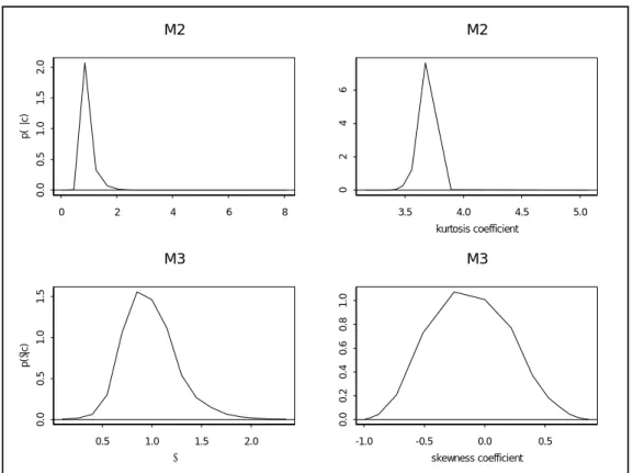
are interpreted as distributional parameters for implicit daily returns distributions, these kurtosis values are representative of returns distributions with a moderate degree of excess kurtosis. The 95% interval estimates cover values forν which translate into kurtosis values which all exceed the value of 3 associated with normality. The modal estimates of the skewness parameter, γ, in M3 and M4, are 0.85 and 0.80 respectively, thereby indicating negative skewness in the implicit daily returns distribution, with (estimates of) the skewness coeﬃcient in (24) of ₋0.253 and ₋0.341 respectively. For M3 in particular, however, the distribution of γ is positively skewed, with a mean estimate close to unity. Moreover, the 95% intervals forγ in both models are very wide, easily covering values for γ which imply either symmetry (γ = 1) or positive skewness (γ > 1), in addition to values implying negative skewness (γ < 1). Some of these numerical results are illustrated graphically in Figure 1, in which the marginal densities for the distributional parameters in models M2 and M3 are reproduced. For M2 the posterior density of the estimated kurtosis coeﬃcient is also presented, providing clear evidence of option-implied excess kurtosis. For M3 the

1 1

An HPD interval is an interval with the speciÞed probability coverage, whose inner density ordinates are not exceeded by any density ordinates outside the interval. The reported intervals have a coverage which is as close to the nominal coverage as possible given the discrete grid deÞned for each parameter.

(20)

0 2 4 6 8 ν 0.0 0 .5 1.0 1 .5 2.0 p( ν |c) M2 3.5 4.0 4.5 5.0 kurtosis coefficient 024 6 M2 0.5 1.0 1.5 2.0 γ 0.0 0 .5 1.0 1 .5 p( γ |c ) M3 -1.0 -0.5 0.0 0.5 skewness coefficient 0.0 0 .2 0.4 0 .6 0.8 1 .0 M3

Figure 1: Implicit Marginal Posteriors for Selected Parameters.

posterior density of the estimated Pearson skewness coeﬃcient is presented in addition to the posterior density for the skewness parameter γ, making clear the fact that all forms of skewness are given high posterior weight, despite the negative mode forγ.

For all six time-varying volatility models,M5 toM10,the option-implied persistence in daily volatility, bδ +ω,b is low in comparison with typical returns-based estimates, ranging from 0.8 to0.84 in terms of point estimates. In addition, the small values estimated for δ

indicate that the volatility process evolves relatively smoothly over the life of the option.12 By construction, the long-run volatility is held Þxed at an annualized value of 0.12 in all cases.

4.5 Model Rankings

4.5.1 Implicit Model Probabilities

Implicit model probabilities are derived from the posterior odds ratios, constructed for each model, M2, M3,. . . , M10,relative to a reference model, M1.DeÞning P(Mk|c) as the

1 2_{Using the EVIEWS program to estimate a}_GARCH₍₁_,₁₎_{models for daily returns on the S&P500 index} for the period 1994 to 1997, estimates similar to those reported in Table 2 are obtained.

(21)

Table 2:

Implicit Marginal Posterior Densities(a)

Model Parameter Mode Mean 95% HPD Interval

M1 σ 0.115 0.115 (0.106, 0.124) M2 σ 0.125 0.125 (0.116, 0.134) ν 0.850 0.934 (0.450, 1.650) M3 σ 0.115 0.115 (0.106, 0.124) γ 0.850 0.986 (0.400, 1.600) M4 σ 0.115 0.115 (0.106, 0.124) ν 0.850 0.919 (0.250, 2.100) γ 0.800 0.891 (0.650, 1.150) M5 δ 0.030 0.031 (0.022, 0.038) ω 0.810 0.810 (0.802, 0.818) M6 v= 5.0 δ 0.030 0.031 (0.022, 0.038) ω 0.810 0.810 (0.802, 0.818) M7 v= 1.0 δ 0.031 0.031 (0.022, 0.038) ω 0.810 0.810 (0.802, 0.818) M8 γ= 0.85 δ 0.040 0.040 (0.031, 0.049) ω 0.760 0.076 (0.751, 0.769) M9 v= 5.0;γ= 0.80 δ 0.030 0.030 (0.022, 0.038) ω 0.780 0.780 (0.771, 0.789) M10 v= 1.0;γ= 0.80 δ 0.030 0.030 (0.022, 0.038) ω 0.780 0.780 (0.772, 0.788)

(a) By conventionσ is reported as an annualized quantity. The distributional parametersνandγrelate to daily returns, whilst the sum of theGARCH parameters,δ andω,measures daily persistence in volatility.

(22)

posterior probability ofMk,the posterior odds ratio for Mk versusM1 is given by P(Mk|c) P(M1|c) = P(Mk) P(M1) × p(c_|Mk) p(c_|M1) (29)

= Prior Odds _× Bayes Factor, fork= 2,3, . . .10,where p(c_|Mk) = Z Σ Z β Z θk L(Σ,β,θk|Mk)p(Σ,β,θk|Mk)dΣdβdθk, (30)

is the marginal likelihood of Mk, with L(Σ,β,θk|Mk) and p(Σ,β,θk|Mk) respectively de-noting the likelihood and prior underMk.The model probabilities are calculated by solving the nine ratios in (29) subject to the normalization

10

X

k=1

P(Mk|c) = 1. (31) The models are then ranked asa posteriori most probable to least probable according to the size of the probabilities. As Σ and β can be integrated out analytically, the marginal likelihood for modelMk reduces to

p(c_|Mk) =h

Z

θk

L(θk|Mk)p(θk|Mk)dθk, (32)

wherehis a constant which is independent of the speciÞcation ofMk. The integral in (32) is that which is computed in the numerical normalization of the posterior density forθk in (7). Hence, the marginal likelihood for each model arises as a natural by-product of the numerical approach adopted, rather than requiring additional computation. Computation of the Bayes factors and implicit probabilities then follows.

Table 3 provides the estimated Bayes factors for the ten models M1 to M10, with M1 used as the reference model. TheÞnal row gives the associated model probabilities, based on equal prior probabilities in (29) for all ten models. There are three notable aspects of the results in Table 3. First, the GST model with constant volatility (M2) is assigned all posterior probability (to two decimal places) in the set of ten alternative models. This is completely consistent with the fact that the option prices have factored in distributional estimates which imply excess kurtosis, as indicated by the results reported in Table 2. Secondly, despite the dominance of theGST model, there is a clear hierarchy amongst the other three constant volatility models, namely M1 is favoured over M4, which is, in turn, favoured over M3.That is, amongst the four constant volatility models, the BS model is ranked second according to posterior probability weight. Thirdly, all six GARCH-based

(23)

Table 3:

Implicit Bayes Factors and Model Probabilities. Entry (i, j) Indicates the Bayes Factor

in Favour ofMj Versus Mi M1 M2 M3 M4 M5 M6 M7 M8 M9 M10 M1 1.00 31400 0.00 0.00 0.00 0.00 0.00 0.00 0.00 0.00 M2 1.00 0.00 0.00 0.00 0.00 0.00 0.00 0.00 0.00 M3 1.00 1200 0.00 0.00 0.00 0.00 0.00 0.00 M4 1.00 0.00 0.00 0.00 0.00 0.00 0.00 M5 1.00 2050 8.3E07 31.30 8.8E09 9.2E25 M6 1.00 40260 0.00 4.3E06 4.5E22 M7 1.00 0.00 106 1.1E18 M8 1.00 2.8E08 3.0E24 M9 1.00 1.1E16 M10 1.00 P(Mk|c) 0.00 1.00 0.00 0.00 0.00 0.00 0.00 0.00 0.00 0.00

models are assigned essentially zero probability when ranked against any of the constant volatility models. The dominance of the constant volatility models reßects the low values in the support of the marginal density forδin theGARCH speciÞcation in (20), which are, in turn, associated with a smoothly evolving volatility process over the life of the option. This results in modelsM5 toM10being eﬀectively overparameterized and, hence, penalized in comparison with the constant volatility models. However, when considered as a separate set, there is a clear ranking across the time-varying volatility models, with the models which impose both excess kurtosis and some negative skewness in the conditional distribution (M9 andM10)favoured most highly, followed by the models with conditional kurtosis only(M6 andM7),followed in turn by the conditional skewness model (M8),then by the conditional normal model (M5).

4.5.2 Out-of-Sample Fit Performance

For modelMk with parameter vectorθk,the residual associated withÞtting the ithoption priceCijf, for moneyness group j, observed on some day f during the hold-out sample is

(24)

deÞned as

resijf = Cijf −b0j−b1jq(zijf,θk)− 4 X l=1 dljDl− G X g=1 ρ_gjCij(f−g) = Cijf −xijf(θk) 0 β_j, (33)

where zijf denotes the option contract speciÞcations associated with Cijf, xijf(θk)0 is a (1_×L) vector of observations at time periodf on theL= 6 +Gregressors associated with

Cijf,and βj is the (L×1)regression vector associated with moneyness groupj. Standard Bayesian distribution theory for a normal linear model yields a multivariate Student t

posterior distribution forβ_j,conditional on θk,with

E(β_j_|θk, c) =βbj and var(β_j_|θk, c) =σb2j h Xj(θk) 0 Xj(θk)i−1,

whereβb_j and σ_b2_j are as deÞned previously in the text. Hence, the posterior distribution for

resijf,conditional onθk,is univariate Student t,with

E(resijf|θk, c) =Cijf −xijf(θk)0βbj (34)

and

var(resijf|θk, c) =σb2jxijf(θk)0

h Xj(θk) 0 Xj(θk) i−1 xijf(θk). (35) The marginal posterior forresijf is thus deÞned as

p(resijf|c) =

Z

θk

p(resijf|θk, c)p(θk|c)dθk. (36) As p(θk|c) is speciÞed numerically over the grid of values for θk used in the numerical normalization ofp(θk|c),the integral in (36) can be estimated by taking a weighted sum of Studenttdensities, with the weights determined byp(θk|c).Given an estimate ofp(resijf|c), a 95%HPD interval forresijf can be calculated. For any given modelMkthere is a residual interval for each option price in the hold-out sample of 984 prices. The proportion of intervals which cover zero is a measure of how well the model Þts out-of-sample, with the bestÞtting model deÞned as the model for which this proportion is the highest.

Results are reported in Table 4 both for the two moneyness groups which are represented out-of-sample: ATM and ITM, and for the full out-of-sample dataset. The number of options in these three groups are respectively 166, 818 and 984. Also included in the lower portion of the table, for all three categories of option, are the average sizes of the bid-ask

(25)

Table 4:

Proportion of 95% Fit Intervals Which Cover Zero;

All Figures are Proportions of the Total Number of Options in Each Contract Group

M1 M2 M3 M4 M5 M6 M7 M8 M9 M10

ATM 0.035 0.078 0.101 0.094 0.022 0.022 0.022 0.032 0.040 0.040

ITM 0.004 0.004 0.004 0.004 0.004 0.007 0.007 0.002 0.002 0.006 All 0.010 0.018 0.024 0.022 0.008 0.010 0.010 0.009 0.010 0.012

Average

Bid-Ask Average Width of

Spread 95% Fit Intervals

M1 M2 M3 M4 M5 M6 M7 M8 M9 M10

ATM $0.87 $0.14 $0.13 $0.14 $0.14 $0.14 $0.14 $0.14 $0.14 $0.14 $0.14

ITM $1.00 $0.06 $0.06 $0.06 $0.06 $0.06 $0.06 $0.06 $0.06 $0.06 $0.06 All $0.98 $0.07 $0.07 $0.07 $0.08 $0.07 $0.07 $0.07 $0.07 $0.07 $0.07

spreads and the average sizes of the 95% intervals, the latter intervals being model-speciÞc. As is evident, the proportion of Þt intervals which cover zero is very small for all models. However, these numbers need to be interpreted with care. The narrow width of the intervals, in particular in comparison with the average bid-ask spreads, means that thisÞt criterion is extremely strict. Only if the model locates the option prices well, that is, if the mean residuals in (34) are very close to zero, does the model have a good chance of producing manyÞt intervals which cover zero. According to this criterion, all models are better able to Þt theATM options, with the proportions being several fold larger than the corresponding proportions for the ITM options. This is despite the fact that the average width of the

ATM Þt intervals is only approximately twice as large as the ITM intervals. Overall, the bestÞtting models are the constant volatility models which allow for either leptokurtosis or skewness or both, followed theBS model. The underperformance of theGARCH models is consistent with their low posterior probability weights.

(26)

4.5.3 Out-of-Sample Predictive Performance

For modelMk,the predictive density for option priceCijf is given by

p(Cijf|c) = Z βj Z σj Z θk p(Cijf|βj,σj,θk, c)p(βj,σj|θk, c)p(θk|c)dβjdσjdθk, (37) wherep(Cijf|βj,σj, c,θk)is a normal density, given the assumption of a normal distribution foruijf in (3). Again, standard Bayesian results enable analytical integration with respect toβ_j and σj such that

p(Cijf|c) =

Z

θk

p(Cijf|θk, c)p(θk|c)dθk, (38) wherep(Cijf|θk, c) is a univariate Studentt density with

E(Cijf|θk, c) =xijf(θk)0bβj (39) and

var(Cijf|θk, c) =σb2j[1 +xijf(θk)0(Xj(θk) 0

Xj(θk))−1xijf(θk)]. (40) The predictive density in (38) can be estimated as a weighted sum of Student t densities, with weights given by p(θk|c). Truncation of p(Cijf|θk, c) at the no-arbitrage lower bound is imposed before averaging over the space of θk. A comparison of (40) with (35) reveals that the Studentt densities used in the mixture which deÞnes the predictive in (38) have a variance which is larger by a factor of σb2_j than the variance of the densities used in the construction of the residual function. This result reßects the standard linear regression structure of the model for the option pricing errors in (3) and mimics the classical prediction results associated with that model.

The estimated predictive density is used to rank the predictive performance of the models in several diﬀerent ways. First, it is used to assign a probability to the observed bid-ask spread associated with the option contract for which Cijf is the market price.13 This calculation is repeated for all option contracts, the predictive probability recorded for modelMkbeing the average of all computed probabilities. Second, with the predictive mode taken as a point predictor of Cijf, the accuracy of each model is assessed in terms of the proportion of predictive modes which fall within the observed bid-ask spreads.14 The same

1 3

With regard to the S&P500 option price data, there is usually only one bid-ask spread associated with a particular option contract, where the speciÞcation of that contract includes the current spot price of the index. For some contracts, however, there are several bid-ask spreads quoted. These spreads are averaged over before being used in the probability calculation described in the text.

1 4

Note that there is a large literature on the market related factors which inßuence the bid-ask spreads associated with option prices. In particular, attempts have been made to explain the way in which the spreads vary across different type of option contracts; see, for example George and Longstaff(1993). On the assumption that these factors do not relate to the nature of the underlying returns process, the observed spreads can be treated as given intervals to which the different models assign varying predicitive probabilities. This assumption may be questionable however; see, for instance, Cho and Engle (1999).

(27)

calculation is performed for the predictive means. Third, the proportion of market prices which fall within the 95% probability interval associated with the estimated predictive, is calculated for each model. As with theÞt results, all calculations are performed for ATM

andITM contracts as well as for all 984 contracts in the hold-out sample, with information on the average bid-ask-spreads and the average width of the model-speciÞc intervals also included. The results for the three diﬀerent contract groupings are reported in Tables 5, 6 and 7 respectively.

As is the case with the Þt results, the predictive results indicate that the constant volatility models with nonnormal distributional speciÞcations, M2, M3 and M4, have the best performance out-of-sample. This is the case for both the ATM and ITM options. In terms of the proportion of times that the point predictors, the predictive mean and mode, fall in the bid-ask spread, the BS model is the next best performer, whilst the GARCH

models tend to have a slightly better predictive performance than theBS model in terms of the observed price falling within the 95% predictive interval. It should be noted, however, that the average width of this interval, in the case of theGARCH models, tends to be larger than the average width associated with theBS intervals, at least for theITM options. The

BS andGARCH models ascribe very similar probabilities to the observed bid-ask spreads, all of which are lower than the corresponding probabilities ascribed by the non-BS constant volatility models. Focussing on the overall results for all out-of-sample options, as reported in Table 7, the average probability ascribed to the bid-ask spread ranges from 31.7% for

M8 and M9 to 33.9% for M2. If the predictive mode is used as a point predictor of the option price, the results in Table 7 show that the probability of predicting an option price within the observed spread ranges from 20.5% for M8 to 26.9% for M4. The predictive mean serves as a more accurate point predictor, with the probability of it falling within the observed spread ranging from 26.6% forM9 to 32.6% forM4.The 95% predictive interval covers the observed market price approximately 70% of the time for all models, with M4 again having the best performance overall according to this criterion. Note however, that whilst the coverage of the predictive intervals appears to be reasonable for all models, the average width of the intervals does exceed the average width of the bid-ask spread, and, hence, could be viewed as being too broad an interval to be useful from a practical point of view.

(28)

Table 5:

Predictive Performance of the Diﬀerent Models (ATM Options)

M1 M2 M3 M4 M5 M6 M7 M8 M9 M10 Predictive Criterion Prob(ba)(a) _0.264 _0.323 _0.326 _0.321 _0.277 _0.278 _0.280 _0.278 _0.276 _0.276 Mode inba(b) 0.300 0.299 0.312 0.314 0.290 0.290 0.288 0.284 0.278 0.283 Mean inba(b) 0.312 0.333 0.340 0.346 0.308 0.312 0.312 0.312 0.308 0.312 Price in 95% I(b),(c) 0.518 0.591 0.613 0.613 0.549 0.549 0.553 0.541 0.541 0.541 Average

Spread 95% Prediction Intervals

M1 M2 M3 M4 M5 M6 M7 M8 M9 M10 $0.87 $1.85 $1.81 $1.81 $1.80 $1.96 $1.96 $1.96 $1.94 $1.93 $1.93

(a) ba = the bid-ask spread. The Þgures reported in this line are the average of the 166 predictive probabilities calculated for each model.

(b) AllÞgures reported are proportions of 166.

(c) The 95% Interval is the interval which excludes 2.5% in the lower and upper tails of the predictive distribution. This interval equals the 95%HPDinterval only for those predictives which are symmetric around a single mode.

(29)

Table 6:

Predictive Performance of the Diﬀerent Models(ITM Options)

M1 M2 M3 M4 M5 M6 M7 M8 M9 M10 $1.00 $1.71 $1.73 $1.75 $1.75 $1.72 $1.73 $1.73 $1.71 $1.71 $1.71

(30)

Table 7:

Predictive Performance of the Diﬀerent Models (All Options)

M1 M2 M3 M4 M5 M6 M7 M8 M9 M10 $0.98 $1.73 $1.74 $1.76 $1.76 $1.77 $1.77 $1.77 $1.75 $1.75 $1.75

(31)

4.5.4 Hedging Performance

Another measure of the performance of alternative option price models is the extent to which the associated hedging errors deviate from zero. In this paper attention is restricted to delta hedges. The delta for theithoption price, in moneyness groupj,observed at time

t,based on the assumption that Mk describes the returns process, is deÞned as

δk=

∂q(zijt,θk)

∂St

. (41)

In computing the hedging errors, the portfolio consists of going short in the option and long in the underlying asset by an amount ofδk shares in the asset, and investing the residual,

Cijt−δkSt, at the risk free interest rate r. At time t+∆t,the hedging error over a time interval∆t,is given by; see Bakshi, Cao and Chen (1997)

Hk=δk h St+∆t−Ster∆t i −hC_ij(t+_∆_t)₋Cijter∆t i . (42)

The posterior distribution of the hedging error in (42) is derived from the posterior dis-tribution for the parameters of model Mk, via δk. In fact, the distribution of Hk is a simple translation of the distribution of δk, obtained by recentering this distribution by

Cij(t+∆t)−Cijter∆t, and rescaling it by St+∆t−Ster∆t. Thus, the hedging error density,

p(Hk|c),can be generated by evaluatingHk,viaδk,at values ofθkin the support ofp(θk|c), and deÞningp(Hk|c)according to the probability weights given by the numerically normal-ized p(θk|c). The model with the hedging error density most closely concentrated around zero is, according to this criterion, the best model.

Two hedge distributions are constructed, based respectively on one-day and Þve-days ahead. The distributions are based on computing the delta hedge on the 15th of December, 1995, and evaluating the hedge error in (42) associated with the portfolio on the next trading day, the 18th of December, 1995, andÞve trading days later, the 22nd of December, 1995. That is,∆t in (42) equals∆t= 1/365 and 5/365 respectively. The calculations are performed on the prices of contracts traded in the pre-3.00pm period which are common to both pairs of trading days. In computing the delta for the BS model, M1,the analytical solution for δk is used; see Hull (2000, p. 312). For the other models, the derivative in (41) is computed numerically. To improve the accuracy of the numerical diﬀerentiation, a control variate is used for these models, based on the diﬀerence between the BS analytical and numerical derivatives. For each value ofθk, the average hedging error over all common contracts is calculated and the density of the (average) hedging error generated as described above.

(32)

The means of the hedging distributions are reported in Table 8, with 95% probability intervals given in parentheses. For the densities which are not symmetric and unimodal, these intervals are only approximately equal to 95%HPDintervals. AllÞgures are expressed in cents. It is clear from the results that the location of the hedging distributions is very similar across models. Only the variability diﬀers across models, with the constant volatility models tending to have the most variable hedging error densities, in particular for one day ahead. The exception to this is the M2 one day ahead hedging error density, which is very tightly concentrated around its mean value. All models produce negative hedging errors one day out and positive hedging errors of a larger magnitude Þve days out. The

GARCH models tend to out-perform the constant volatility models one day out, at least in terms of producing hedging errors of a smaller magnitude. However, there is no clear ranking of the models in terms of the Þve days ahead hedging errors. Most notably, none of the intervals reported in Table 8 cover zero. This can be interpreted as meaning that all models considered are misspeciÞed when it comes to hedging; see also Bakshi, Cao and Chen (1997), who obtain similar qualitative results. However, whether the observed hedging errors are signiÞcant from an economic point of view is unclear. The hedging errors range in magnitude from approximately 13 to 52 cents, whilst from Table 1 it can be seen that the option prices in the out of sample dataset themselves range from an average price of $20.61forATM options to an average price of$70.38forITM options. Viewed in relation to the magnitude of the option prices, these hedging errors do not seem to be substantial.

5 Conclusions

This paper has developed a Bayesian approach to the implicit estimation of returns models using option-price data. In contrast to existing classical work, the Bayesian method takes explicit account of both parameter and model uncertainty in option pricing. The paper also represents a signiÞcant extension of other Bayesian work on option pricing, with a full set of alternative parametric models for returns estimated and ranked using option-price data. Risk-neutral valuation under nonnormal distributional speciÞcations is implemented in a direct and computationally eﬃcient manner.

The results of applying the methodology to 1995 option price data on the S&P500 index show that no one parametric model is ranked highest according to all criteria. The GST

model clearly dominates all other models, including the BS model, in terms of posterior probability, this result being consistent with the excess kurtosis which is estimated from the option prices. The evidence in favour of option-implied skewness is weaker. However,

(33)

ignor-Table 8:

Hedging Performance of the Diﬀerent Models (cents): One Day and Five Days Ahead Means of Hedging Error Densities and 95% Intervals

One Day Ahead Five Days Ahead Mean 95% Interval Mean 95% Interval

M1 -20.195 (-23.500, -16.500) 51.005 (51.001, 51.023) M2 -14.108 (-14.110, -14.106) 51.677 (51.640, 51.700) M3 -16.329 (-17.000, -12.500) 52.001 (51.500, 52.080) M4 -17.308 (-17.900, -16.500) 51.573 (51.000, 52.300) M5 -13.682 (-13.720, -13.580) 52.056 (52.080, 52.120) M6 -14.378 (-14.470, -14.370) 51.983 (51.970, 52.020) M7 -14.454 (-14.500, -14.430) 51.997 (51.960, 51.980) M8 -13.924 (-13.930, -13.830) 52.310 (52.270, 52.320) M9 -14.234 (-14.270, -14.230) 51.116 (51.114, 51.118) M10 -13.501 (-13.499,-13.502) 51.677 (51.610, 51.690)

ing the impact of risk factors on the option-based estimates of the higher order moments, it can be concluded that the option prices have factored in more negative skewness than is evident in the symmetric distribution observed for daily S&P500 returns during 1995. This result is consistent with the idea that, since 1987 in particular, option market participants have factored in a larger probability of negative returns than would be predicted by a nor-mal returns distribution; see, for example, Bates (2000). Overall, the constant volatility models which allow for either excess kurtosis or negative skewness in returns, or both, tend to have the best out-of-sample Þt and predictive performance, with the BS model being ranked lowest in the constant volatility model set on nearly allÞt and prediction criteria. TheGARCH models are assigned virtually zero posterior probability when ranked against the constant volatility models, as well as having an out-of-sample Þt and predictive per-formance which is usually dominated by that of the constant volatility models, including theBS model. This inability of the GARCH models to capture the behaviour of S&P500 option prices is somewhat consistent with the poor predictive power reported by Chernov and Ghysels (2000) forGARCHoption pricing models, as based on an earlier sample period for the same option price series. In terms of hedging, all of the models appear to be equally misspeciÞed, although the magnitudes of the hedging errors, relative to the magnitude of the option prices, are very small.