Probabilistic methods for high dimensional signal processing

dimensional signal processing

Jean-Baptiste Regli

A dissertation submitted in partial fulfillment of the requirements for the degree of

Doctor of Philosophy of

University College London.

Department of Statistical Science University College London

I, Jean-Baptiste Regli, confirm that the work presented in this thesis, except as noted herein, is my own. Where information has been derived from other sources, I confirm that this has been indicated in the work.

This thesis investigates the use of probabilistic and Bayesian methods for analysing high dimensional signals. The work proceeds in three main parts sharing similar objectives. Throughout we focus on building data efficient inference mechanisms geared toward high dimensional signal processing. This is achieved by using probabilistic models on top of informative data representation operators. We also improve on the fitting objective to make it better suited to our requirements.

Variational Inference

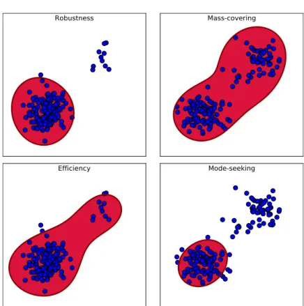
We introduce a variational approximation framework using direct optimi-sation of what is known as the scale invariant Alpha-Beta divergence (sAB divergence). This new objective encompasses most variational objectives that use the Kullback-Leibler, the Rényi or the gamma divergences. It also gives access to objective functions never exploited before in the context of variational inference. This is achieved via two easy to interpret control pa-rameters, which allow for a smooth interpolation over the divergence space while trading-off properties such as mass-covering of a target distribution and robustness to outliers in the data. Furthermore, the sAB variational objective can be optimised directly by re-purposing existing methods for Monte Carlo computation of complex variational objectives, leading to es-timates of the divergence instead of variational lower bounds. We show the advantages of this objective on Bayesian models for regression problems.

Roof-Edge hidden Markov Random Field

We propose a method for semi-local Hurst estimation by incorporating a Markov random field model to constrain a wavelet-based pointwise Hurst estimator. This results in an estimator which is able to exploit the spatial regularities of a piecewise parametric varying Hurst parameter. The point-wise estimates are jointly inferred along with the parametric form of the underlying Hurst function which characterises how the Hurst parameter varies deterministically over the spatial support of the data. Unlike recent Hurst regularisation methods, the proposed approach is flexible in that ar-bitrary parametric forms can be considered and is extensible in as much as the associated gradient descent algorithm can accommodate a broad class of distributional assumptions without any significant modifications. The potential benefits of the approach are illustrated with simulations of vari-ous first-order polynomial forms.

Scattering Hidden Markov Tree

We here combine the rich, over-complete signal representation afforded by the scattering transform together with a probabilistic graphical model which captures hierarchical dependencies between coefficients at different layers. The wavelet scattering network result in a high-dimensional repre-sentation which is translation invariant and stable to deformations whilst preserving informative content. Such properties are achieved by cascad-ing wavelet transform convolutions with non-linear modulus and averag-ing operators. The network structure and its distributions are described using a Hidden Markov Tree. This yields a generative model for high-dimensional inference and offers a means to perform various inference tasks such as prediction. Our proposed scattering convolutional hidden Markov tree displays promising results on classification tasks of complex images in the challenging case where the number of training examples is extremely small. We also use variational methods on the aforementioned model and leverage the objective sAB variational objective defined earlier

In the last decade the machine learning and signal processing communities have seen game changing improvements and this has caused the devel-opment of many applications in both academia and industry. The work presented in that thesis leverage those methods and improve on top of them.

Recent machine learning methods tend to rely on a having access to a vast amount of correctly annotated examples to perform prediction and “extrapolation“. This paradigm is not always true and this work focuses on reducing this dependency. We propose methods allowing to perform accurate complex image classification based on only a very limited num-ber of training examples. This type of methods can prove to be useful in domains where collecting examples is costly (medical studies, physic experiments, rare events...). Those methods also heavily relies on correct annotations. We here develop methods to alleviate that need. This types of methods are valuable in situation where a perfect oracle —i.e. person able to produce annotations— does not exist. This is the case for example for medical image analysis, in analysis of spatial imagery. Those two improve-ments reduce the cost of using machine learning by reducing the need for big highly curated datasets.

Another pitfall of currently used methods is the lack of measure of uncertainty on the prediction made. In this work we develop methods

al-lowing estimation of the quality of the prediction. This information can be leverage in systems where a wrong decision would have high conse-quences (medical, military...) to trigger more analysis. This uncertainty can also be used by an higher level control/learning algorithm to explore more the training space in the direction of that uncertainty.

I would like to express my deepest gratitude to my supervisors Ricardo Silva and James Nelson, UCL Statistical Science department, DSTL, and my family.

1 Introduction 21 1.1 Overview . . . 21 1.2 Publications . . . 22 1.3 Motivation, contribution, and related work . . . 22

I

Background

29

2 Signal representation 31

2.1 Intuition: . . . 33 2.2 Formalisation: . . . 36 2.3 Scattering transform . . . 40

3 Probabilistic Graphical Models 57

3.1 Bayesian Networks: . . . 58 3.2 Markov Models: . . . 63 3.3 Variational inference . . . 67

II

Flexible Variational Inference

71

4 Alpha-Beta variational Inference 73

4.1 Introduction . . . 74 4.2 Background . . . 75 4.3 Scale invariant AB Divergence . . . 79

4.4 sAB-divergence Variational Inference . . . 86

4.5 Experiments . . . 90

4.6 Conclusion . . . 93

III

Roof-Edge hidden Markov Random Field

97

5.2 Background . . . 102

5.3 Parameterised MRF Hurst estimation . . . 105

5.4 Experiments . . . 107

5.5 Conclusion . . . 110

IV

Scattering Hidden Markov Tree

115

6.2 Background . . . 119

6.3 SHMT model . . . 121

6.4 Learning the tree parameters . . . 131

6.5 Classification . . . 138

6.6 Experiments . . . 140

6.7 Conclusion . . . 147

7 Variational Scattering Hidden Markov Tree 149 7.1 Introduction . . . 150

7.2 Background . . . 151

7.3 Structured mean field for HMTs . . . 152

7.4 AB-variational objective for HMTs . . . 160

7.5 Experiments . . . 162

V

Conclusions

169

VI

Annexes

177

.1 AB variational Inference: . . . 179

.2 Extension by continuity of the sAB-divergence . . . 180

.3 Special cases of the sAB-divergence . . . 184

.4 Robustness the sAB-divergence . . . 186

.5 sAB-divergence Variational Inference . . . 187

.6 Experiments . . . 191

2.1 Example of high dimensional signals. . . 32

2.2 Example of signal translation invariance. . . 34

2.3 Example of stability to deformations. . . 35

2.4 Example of limited invariance to rotation. . . 36

2.5 Convolutional neural network. . . 40

2.6 Representation of the Morlet wavelet. . . 42

2.7 Scattering convolutional network architecture. . . 48

2.8 Frequency decreasing scattering convolution network. . . 52

2.9 Samples from the MNIST handwritten digits recognition dataset. . . 55

3.1 A simple Bayesian network. . . 59

4.1 Illustration of the robustness/efficiency and mass-covering/mode-seeking properties . . . 76

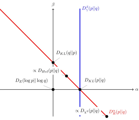
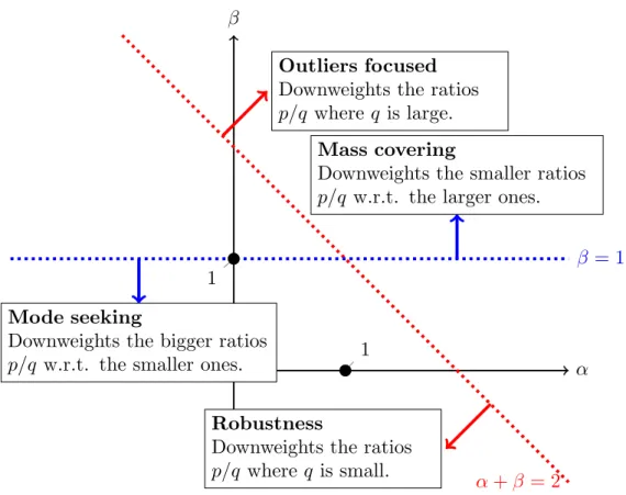
4.2 Mapping of the (α,β) space . . . 83

4.3 AB divergence parameter influence . . . 86

4.4 Approximation of a mixture of 2 skewed densities with AB-variational objective. . . 87

4.5 AB-divergence — Toy dataset regression experiment. . . 92

5.1 Hurst Estimation — ”Hip” Brownian surface. . . 109

5.2 Hurst Estimation — ”Pavillon” Brownian surface. . . 110

5.3 Hurst Estimation — ”Grambrel” Brownian surface. . . 111

5.5 Hurst Estimation — Fractional Brownian surfaces. . . 113

5.6 Hurst Estimation — Absolute error histograms. . . 114

6.1 Scattering transform tree. . . 119

6.2 Scattering hidden Markov tree. . . 122

6.3 K populations - Experiment 1. . . 126

6.4 K populations - Experiment 2. . . 127

6.5 Persistence - Experiment 1. . . 129

6.6 SAS sonar raw image. . . 144

6.7 Sample of seabed patches. . . 144

6.8 Sample of ripple patches. . . 145

6.9 Segmentation of a sonar imagery. . . 147

7.1 Variational scattering hidden Markov tree. . . 156

7.2 Sample of seabed patches. . . 166

7.3 Sample of ripple patches. . . 166

4.1 AB-divergence — Toy dataset regression experiment . . . 91 4.2 AB-divergence — MNIST classification experiment . . . 93 4.3 AB-divergence — UCI datasets regression experiment . . . . 94 5.1 Hust estimation — HMRF regularisation . . . 108 6.1 SHMT — Persistence - Experiment 2. . . 129 6.2 SHMT — Mnist One shot “One vs All” classification

experi-ment . . . 141 6.3 SHMT — Mnist One shot multiclass classification experiment 142 6.4 SHMT — Seabed classification performance. . . 145 7.1 SHMT — Mnist One shot “One vs All” classification

experi-ment 2 . . . 164 7.2 SHMT — Mnist One shot multiclass classification experiment 164 7.3 SHMT — Seabed classification performance. . . 166

Introduction

1.1

Overview

This thesis explores several methods to perform Bayesian inference and analysis on high dimensional signals. More specifically we are interested in extracting knowledge from a small number of realisations of a po-tentially corrupted signal whilst —ideally— being able to quantify the uncertainty over this inferred information.

Those constraints are motivated by an application to a problem sug-gested by the Defence Science and Technology Laboratory (Dstl). They are interested in methods to perform underwater mine detection in sonar images. By nature, the access to training examples is limited. And the reliability of the detection has to be quantifiable due to how catastrophic a false negative could be.

Throughout the thesis we explore how Probabilistic Graphical Models (PGMs) and signal representation methods can be combined. And used to perform inference that is both data efficient and might allow to quantify uncertainty.

1.2

Publications

The thesis structure is based on the following published or soon to be published work.

Variational Inference

• J.-B. Regli and R. Silva. “Alpha-Beta Divergence For Variational In-ference”. In: arXiv preprint arXiv:1805.01045(2018)

Roof-Edge hidden Markov Random Field

• J.-B. Regli and J. Nelson. “Piecewise parameterised Markov random fields for semi-local Hurst estimation”. In: Signal Processing Conference (EUSIPCO), 2015 23rd European. IEEE. 2015, pp. 1626–1630

Scattering Hidden Markov Tree

• J.-B. Regli and J. Nelson. “Scattering convolutional hidden Markov trees”. In: Image Processing (ICIP), 2016 IEEE International Conference on. IEEE. 2016, pp. 1883–1887

Note that, to this day, some chapters are still unpublished.

1.3

Motivation, contribution, and related work

This section provides a brief introduction to the main themes of this thesis, motivates the research objectives, and points out related work.

1.3.1

Alpha Beta Variational Inference

Modern probabilistic machine learning relies on complex models for which the exact computation of the posterior distribution is intractable. This has motivated the need for scalable and flexible approximation methods. Re-search on this topic belongs mainly to two families, sampling based meth-ods constructed around Markov Chain Monte Carlo (MCMC) approxima-tions [73], or variational inference (VI) [49]. In this work, we focus on the latter, although with the aid of Monte Carlo methods.

Contribution.We propose a variational objective to simultaneously trade-off effects of mass-covering, spread and outlier robustness. This is done by developing a variational inference objective using an extended version of the alpha-beta (AB) divergence [107], a family of divergence governed by two parameters and covering many of the divergences already used for VI as special cases. After reviewing some basic concepts of VI and some useful divergences, we extend it to what we will call the scale invariant AB (sAB) divergence and explain the influence of each parameters. We then develop a framework to perform direct optimisation of the divergence mea-sure which can leverage most of the modern methods to enmea-sure scalability of VI. Finally, we demonstrate the interesting properties of the resulting approximation on regression tasks with outliers.

Related work.The quality of the posterior approximation is a core ques-tion in variaques-tional inference. When using the KL-divergence [2] averaging with respect to the approximate distribution, standard VI methods such as mean-field underestimate the true variance of the target distribution. In this scenario, such behaviour is sometimes known as mode-seeking [75]. On the other end, by (approximately) averaging over the target distribu-tion as in Expectadistribu-tion-Propagadistribu-tion, we might assign much mass to low-probability regions [75]. In an effort to smoothly interpolate between such behaviours, some recent contributions have exploited parameterised fam-ilies of divergences such as the alpha-divergence [75, 112, 157], and the Rényi-divergence [158]. Another fundamental property of an approxima-tion is itsrobustness to outliers. To that end, divergences such as the beta [42] or the gamma-divergences [84] have been developed and widely used in fields such as matrix factorisation [96, 108]. Recently, they have been used to develop a robust pseudo variational inference method [162].

Roof-Edge hidden Markov Random Fields

The Hurst parameter determines the spectral decay rate of a process with a power-law spectrum. Since such a simple relationship is ubiquitous in

many signal and image processing areas and beyond [58, 63] Hurst estima-tion continues to enjoy many, and disparate, applicaestima-tions including Finance [126], signal/image denoising [83], clutter suppression [99], segmentation [122], the analysis of ECG signals [124, 134], internet traffic flow [58], image texture [53], and turbulence data [85].

The interconnection between wavelets and self-similar processes is a powerful, if not, surprising one. The self-similarity explicitly built into the wavelet basis functions via the two-scale, or refinement, relations provides a natural representation in which to study processes that exhibit power-law behaviour. However, the localised nature of wavelets also facilitates a localised estimation of the Hurst parameter.

Contribution.Since it is reasonable to assume that an image of interest may comprise multiple textures, it is appropriate to consider a piecewise smoothly varying Hurst parameter H= H(r), for r over some subregion of R2. Furthermore, we let the way in which this Hurst function varies over space be governed by some parametric form H=φ(r;θ) with model

parameters θ. We would expect these parameters to be fairly constant over

certain subregions of the image domain where the image texture is homo-geneous. We allow the spatial support to accommodate multiple textures with a suitable partitioning of disjoint subregions. In each subregion, the

θare assumed constant (or have very small, smooth variations). However,

between subregion boundaries, it is allowed to change arbitrarily. As a con-sequence the Hurst parameter itself will vary smoothly inside a partition and vary arbitrarily across the respective subregions. We here propose a model and inference scheme that exploits this piecewise parametric out-look. The framework utilises a Markov random field prior to constrain, or penalise, the magnitude of parameter variation over the image.

Spatial regularisation of Hurst estimation has been recently consid-ered as a means to exploit prior knowledge about the spatial smoothness of the Hurst parameter [140]. However, the method was based on the

generalised lasso and assumed only a piecewise constant varying Hurst parameter. In contrast our model, and corresponding gradient-descent-like algorithm, are more flexible. The framework can accommodate many different kinds of distributional assumptions and arbitrary models that de-scribe how the Hurst parameter varies deterministically in space. On the other hand, the generalised lasso Hurst estimator simply penalises the `1

-norm of the Hurst parameter spatial derivatives (of some specified order). Therefore, along with a fixed Gaussian assumption on the data, the spa-tial derivatives of the Hurst parameter are assumed to be Laplacian and it is difficult to incorporate other distributional assumptions without mak-ing wholesale changes to the inference scheme. Other assumptions would necessitate a change in inference strategy (if one existed). Furthermore, unlike the method proposed here, the lasso inference does not obtain any estimate of the underlying parametric form of the Hurst ‘function’.

Related work.Although there are works, such as those based on the mul-tifractal formalism [82, 88], that describe how regularity varies across an image, less attention has been paid to the case where the main interest is to obtain pointwise estimates of a Hurst parameter that is allowed to vary as a smooth, deterministic function. Such a scenario could, for example, present itself in image processing when the texture of an object of interest varies gradually over its spatial support in some assumed manner. In turn this would facilitate tasks such as feature extraction, segmentation, and change detection. Likewise, existing adaptive denoising methods, which are currently based on a piecewise constant Hurst parameter [140], could also be extended to include more general Hurst functions that vary as piecewise parametric functions.

[99] leverage the expressiveness of the dual tree complex wavelet trans-form [76], to pertrans-form efficient global Hurst estimation and apply it to ripple suppression for underwater mine detection.

Scattering Hidden Markov Tree

The standard approach to classify high dimensional signals can be ex-pressed as a two step process. First the data are projected in a feature space where the task at hand is simplified. Then prediction is done using a sim-ple predictor in this new representational space. The mapping can either be hand-built —e.g. Fourier transform, wavelet transform— or learned. In the last decade methods for learning the projection have drastically improved under the impulsion of the so called deep learning. Deep neural networks —often enriched by convolutional architecture— have been able to learn very effective representations for a given dataset and a given task [33, 102, 105]. Such methods have achieved state of the art on many standard prob-lems [114, 115] as well as real world applications [150].

However deep learning methods are only efficient when we have ac-cess to a vast quantity of training examples [97]. But in some cases, such as in medical or defence applications for example, datapoints are rare or us-ing an expert for hand-labellus-ing them is time-consumus-ing, costly or subjec-tive. Hence in situations where training examples are expensive to collect, learning has to be performed on smaller datasets. In that case using a fixed, hand crafted set of filters seems to be one of the best solution [56]. Recently Mallat [168] introduced the scattering transform— a fixed bank of wavelet filters used to generate data representation in a convolutional neural net-works like architecture. This representational approach was used together with a support vector machine classifier (SVM) and achieved close to state of the art performance on a number of standard datasets [94]. Moreover, it has been shown that this method performs very well on a relatively smaller numbers of training examples [130] —i.e. less that 1000 training samples. Contribution.We propose to model Mallat’s scattering convolutional net-work [94] using hidden Markov trees. This combines a recently proposed deterministic, analytically tractable transformation inspired by deep con-volutional networks with a probabilistic graphical model. It creates a

po-tentially powerful probabilistic tool to handle high-dimensional prediction problems. Unlike previous work on hidden Markov wavelet trees, the use of scattering transforms allow us to exploit their full range of invariances. However, it also compels us to adapt the HMT model to non-homogeneous, non-regular trees. In contrast to simply passing the raw scattering coeffi-cients into a classifier, our proposed framework captures dependencies be-tween different layers in a generative probabilistic model. Moreover, unlike standard classification, once trained our model can tackle not only predic-tion problems but also other inference tasks such as generapredic-tion, sensitivity analysis, etc and can also outperform SVMs when only a very small num-ber of training examples are available.

Related work.When only a very small number of training samples are available one-shot learning [79] generative classification methods achieve significantly better results than discriminative models [61], however they require pre-training. Generative probabilistic graphical models have been successfully constructed for various wavelet transforms; in particular, Hid-den Markov trees have been used to model the depenHid-dencies between the wavelet coefficients [43, 57, 71].

Thesis structure

We begin by introducing some necessary concepts and notations in Part I. This includes a brief introduction to signal representation with a focus on elements used in the remainder of the thesis associated to some element more specific to this work in Chapter 2 and probabilistic graphical models in Chapter 3.

Part II – Flexible Variational Inference

Chapter 4 defines a new objective for variational inference. It defines a new objective based on a flexible divergence measure family allowing more complex approximation properties.

Part III – Roof-Edge hidden Markov Random Field estimation

Chapter 5 provides one way of combining signal representation and prob-abilistic graphical models to perform high dimensional signal analysis. Those tools are used to perform image segmentation based on the local value of the Hurst coefficient.

Part IV – Scattering Hidden Markov Tree

Chapter 6 introduces a novel method to combine scattering transform and probabilistic graphical model to describe a signal. Chapter 7 extends that framework from exact inference to approximate inference using the objec-tive defined in Chapter 4.

Part V – Conclusions

We finally conclude, and discuss potential future work and recent develop-ments related to this work.

Background

Signal representation

This chapter introduces the need for signal representation step prior to per-forming inference. We then review the desired properties of the operator projecting the signal into that representational space. After reviewing some classical representation operators, we introduce the scattering transform, a representation operator that will be used later in the thesis.

Let us consider the problem of inferring the value of a latent variable ygiven the observed signalxnew. Though some of the frameworks detailed in this documents are more general, we will mainly focus on signals such that x=_{x[1]. . .x[d]_} with d_≈106, x[.]_∈R and y_∈N. Let us call f the inference function and {x_i, ˆyi= f(xi)}i≤N the N sampled potentially noisy training values. Example of such signals and latent variables are, speech waveforms of different words, digital photographs of different objects but also electrocardiograms of various heart states, sonar images of multiple features and many others.

0 0.5 1 1.5 2 2.5 3 3.5 4 4.5 −0.6 −0.4 −0.2 0 0.2 0.4 0.6 0.8

Figure 2.1: Example of high dimensional signals.

Left: Waveform of a flute recording.

Bottom: Image of a Mandrill.

A naive solution to this problem would be to infer the value of the latent variables for a new realisation xnew by looking at its neighbours in the signal space Rd. In essence this approach is similar to the K-Nearest Neighbours (KNN) [26]. Though this type of methods are effective for low-dimensional problems [9], they show limitations in high dimensional cases [48]. Indeed, the number of samples required to find a neighbour within a given distance to a new realisationxnew grows exponentially with the number of dimensions. This issue is known in the statistical learning community as the curse of dimensionality [120] and prevent the use of neighbour based methods directly on high dimensional signals.

One can assume the signal x to belong to a manifold, say Ω, of Rd. This yields two types of problems. Either the subsetΩ is low dimensional orΩ is also high dimensional. In the former, one can mitigate the effect of the curse of dimensionality once the manifold has been isolated. The task at hand is thus a manifold learning problem [86, 119] or a sparse dictio-nary representation problem [68]. For some signals however, the manifold

Ω is also expected to be of high dimensionality. In this case, in order to simplify the inference task, one can only try to reduce the volume of the signal space without losing the crucial information required to characterise it. This can be achieved by reducing the volume of Ωalong the invariants in the input signal space [168]. In the remainder of the document we focus on this latter case.

In the remainder of this chapter we focus on designing a mapping, say

Φ, which project the signal into a new space where the inference task is simplified. This space should not only capture the main information and discriminatory content in the data but it should also remain stable with respect to appropriate transformations and deformations. Before provid-ing a formal mathematical description of this mappprovid-ing, it is instructive to consider the following intuitive examples.

2.1

Intuition:

We here provide an intuition of the desired properties of what we will refer as a “good” signal representation. To that end, it is informative to consider the example of image classification. And more specifically to focus on the elements ensuring good generalisation capacities. Using this approach, one can intuit the following properties for the projectionΦ:

infer-ence. This means ensuring that Φpreserves separability between the different clusters.

• The mapping also has to be — partially— invariant to translations. Indeed, the information carried by a signal remains the same under limited shifts (see Figure 2.2). This means the transformation Φ has to provide close, if not equal, outputs for shifted versions of the same signal.

Figure 2.2: The information contained in a signal is invariant to local translations.

Left: Original signal.

Bottom: Translated version of the signal containing the same informa-tion.

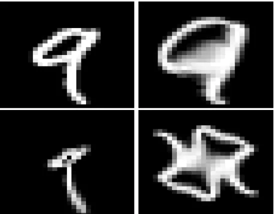
• To some extent the mapping also has to be stable under deforma-tions. Again, the information contained in a signal remains similar if it has undergone —limited— deformations. Yet if the amplitude of the morphings are too important with regard to the information contained in the signal, then critical features of the signal can be lost (see Figure 2.3). This implies that to a certain degree the projections of morphed realisations of the same signal should be mapped to a same region of the representational space. As opposed to translation, however, one does not want complete invariance to deformation but rather continuous response to it. This is to ensure that the

repre-sentation created is still informative enough and does not project all inputs to the same region of the space, but instead provide a smooth response to deformations.

Figure 2.3: The information contained in a signal is stable to deformations limited in amplitude.

Top Left: Original signal.

Top Right: Very lightly deformed version of the signal still containing the same information.

Bottom Left: Lightly deformed version of the signal still containing the same information.

Bottom Right: Highly deformed version of the signal. The information is lost.

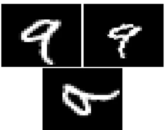
• Again to a certain degree, the projection has to be invariant to rota-tions. Only limited invariance to rotation is wanted because excessive rotation applied to the original signal can be destructive for the in-formation carried (see Figure 2.4). Solutions based on the method described in this document exist [130, 142]. The methods described in Part IV do not incorporate this invariance but could directly be

extended to do so.

Figure 2.4: The information contained in a signal is to a certain extend invariant to rotation.

Top Left: Original signal.

Top Right: Lightly rotated version of the signal still containing the same information.

Bottom Left: Highly rotated version of the signal. The information is lost.

2.2

Formalisation:

Throughout this section, attention is restricted to signals represented by square-integrable d-dimensional functions over the real numbers, namely x_{∈ L}2(Rd). For sake of simplicity, inference is reduced to categorical vari-able such that f is now a classification function. Let us define the function g and h such that f =h◦g. The function g denotes the soft classification function, i.e. g(x)_∈ RK where K is the dimension of the mapping space, and represents the distance to the separating surface. The labelling func-tion h is defined such that y =h_◦g(x) is now the label associated to a

signal x.

To be informative enough, a representation must preserve separability between elements of different classes. This is encapsulated by the following definition.

Definition 2.2.1. (Separability preservation)

A representation Φ preserves separability if all elements of two different classes are distant of at least a margin C in the representation space,

∀x,x0∈Rd ∃C∈RK s.t. h◦g(x)6=h◦g(x0) ⇒ kΦ(x)−Φ(x0)k ≥C−1 where K is the dimension of the mapping space.

Translations in the input space should not affect the representation. Let L_(.) denote the translation operator for the function in _L2(Rd), i.e. for x_∈

L2_(Rd_{) and u,c∈R}d_×Rd _L

cx(u) =x(u−c). A mappingΦis translation invariant —respectively canonical translation— if it projects a translated signal to the same point as its original version.

Definition 2.2.2. (Translation invariance)

LetH be an Hilbert space, an operatorΦ:L2_(Rd_{)→ His translation invariant}

if:

∀c_∈Rd and _∀x_{∈ L}2(Rd) Φ(Lcx) =Φ(x).

Definition 2.2.3. (Canonical translation invariant)

Let_Hbe an Hilbert space, an operator Φ:_L2(Rd)_{→ H} is canonical translation invariant if:

For the standard representation operators, instabilities to deformations are known to appear —especially at high frequencies. To prevent this, one would like the representation to be non-expansive.

Definition 2.2.4. (Non-expansive representation) A representationΦis non-expansive if,

∀x,x0_{∈ L}2(Rd) _kΦ(x)₋Φ(x0)_{k ≤ k}x₋x0_k.

The local stability to deformations of a non-expansive operator can be expressed as its Lipschitz continuity to the action of deformations close to translations [168]. Such a diffeomorphism can be expressed as a canonical translation,

Lτ :L2(Rd)→ L2(Rd)

x _→x((.)−τ(.))

whereτ(u)∈Rd is a displacement field — i.e. a transformation associating a displacement vector to each point of the signal.

Definition 2.2.5. (Lipschitz continuous)

A non expansive operator Φ is said to be Lipschitz continuous to the action of

C2 _{diffeomorphisms if for any compact Ω⊂R}d _{there exists C such that for all}

f ∈ L2_(Rd_{)supported inΩand all}

τ∈ C2(Rd), kΦ(x)₋Φ(Lτx)kH ≤Ckxk sup u∈Rd|∇ τ(u)|+ sup u∈Rd| Hτ(u)_| ! (2.1)

where∇τ(u) is a matrix whose norm|∇τ(u)|measures the deformation ampli-tude at point u, Hτ(u) is the Hessian matrix of the deformation and its sup-norm

Hence such a Lipschitz continuous operator Φ is almost invariant to deformations byτ(.), up to the first and second order deformation terms. Equation 2.1 also implies that Φ is invariant to global translations but this is already enforced by the translation invariance requirement from Defin-ion 2.2.2.

This part and more precisely Section 2.3 introduces an analytically tractable, deterministic wavelet based transformation fulfilling all the prop-erties mentioned in this section.

2.2.1

State of the art:

A common representational method is the modulus of the Fourier trans-form [21]. To a certain extent, this operator is intrans-formative enough to allow discrimination between different types of signals [133]. It is also translation invariant [7]. It is well-known, however, that those operators present insta-bilities to deformation at high frequencies [14] and thus are not Lipschitz continuous to the action of diffeomorphisms.

Another popular representation method is the wavelet transform [27]. Projection of a signal into the wavelet space also provides a representation suitable for inference [52]. We define the wavelet operator by the following set of convolutions, Wx=     x_∗φ x_∗ψλ     →averaging part

→high frequency part

The averaging part expresses is obtained by convolving the signal with a low frequency filter. By grouping high frequencies into dyadic packet, wavelet operators are stable to —small— deformations [121]. However only the averaging part of a wavelet is invariant to translation. Thus wavelets themselves are known to be non-invariant to translations.

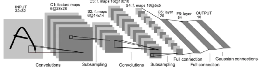
Another popular signal representation method are the convolutional neural networks [33]. As opposed to the two methods mentioned previ-ously, those operators are not fixed but learned from the data [70]. Over the past decade they have provided state of the art results on many standard classification tasks, on image datasets such as MNIST [151], CIFAR [114] and ImageNet [115] as well as on speech processing problems such as TIMIT [111]. Those good results are used to advocate that those networks are learning “good” representations. There is, however, no mathematical formalisation of this intuition and it seems that in certain cases they learn representation of the data that are, for example, not invariant to deforma-tions [131, 137].

Figure 2.5: Convolutional neural network with 3 convolution/sub-sampling layers and 3 fully connected layers. Image from [45].

2.3

Scattering transform

In this section we describe the construction of a mathematical operator —the scattering transform (ST) [168]— designed to generate what we de-fined earlier as an interesting representation of signal (see Section 2.2). This operator projects the signal’s informative content into scattering de-composition paths, computed by cascading wavelet/modulus operators through an architecture similar to a Convolutional Neural Network (CNN) where the synaptic weights would be given by a wavelet operator instead

of learned.

The remainder of this chapter is organised as follows. First, Sec-tion 2.3.1 defines the scattering operators. Second, SecSec-tion 2.3.2 describes how those operators can be stacked to create a Scattering Convolutional Network (SCN), an architecture comparable to a fixed filter CNNs. Then Section 2.3.3 reviews some important properties of the SCNs. And finally, Section 2.3.7 presents how the scattering transform is usually used in clas-sification tasks.

2.3.1

Scattering coefficients:

In this section we focus on the details involved to build an operator ful-filling the properties defined in Section 2.2. As seen in Section 2.2.1, the wavelet wavelet transform already possess some of those properties. Furthermore it can be combined with simple mathematical operators to acquire the missing desired properties.

A two-dimensional directional wavelet is obtained by scaling and ro-tating a mother wavelet ψ acting as a single band-pass filter. Let G be a discrete, finite rotation group of R2, multi-scale directional wavelet filters are defined for any scale j∈Z and rotationr∈G by,

ψλ(u) =ψ2j_r(u) =22jψ(2jr−1u). (2.2) To simplify the notations, we set λ=λ(j,r) =d 2jr ∈ Λ=d G×Z.

A bank of dilated and rotated filters — a wavelet bank of filters— is obtained by simply evaluating Equation 2.2 for different values of λ∈Λ. This bank of filter has no orthogonality properties amongst each other [50]. The wavelet transform projects the signal x into a representational space using such a bank of filters yielding {x_∗ψλ(u)}λ. This generates a

multi-scales and multi-orientations representation of the input signal.

The Morlet wavelet is an example of Wavelet. The mother wavelet ψmorlet is given by,

ψmorlet(u) =C1(eiu.ξ−C2)ekuk

2_/2

σ2_,

where C1, ξ and σ are meta-parameters of the wavelet and C2 is adjusted

so that R

ψ(u)du =0. Figure 2.6 shows a Morlet wavelet for ξ =3π/4, σ=0.85 andC1=1. The complete family is obtained by evaluatingψmorlet at different scales and orientations as described in Equation 2.2.

Figure 2.6: Representation of the complex Morlet wavelet for ξ =3π/4, σ=0.85

andC1=1. Redrawn after [113].

Left: Real part of ψ.

Center: Imaginary part of ψ. Right: Fourier modulus_|ψˆ|.

As opposed to the Fourier sinusoidal waves, wavelets are operators stable to localL2 _{deformations as they can be expressed as localised} wave-forms [50]. However, as wavelet transform computes a convolution with a wavelet basis, the resulting transform is a translation covariant opera-tor [121].

To make a translation covariant operator translation invariant, one can introduce a non-linearity in the processing pipeline. However one need to

make this non linearity such that it does not remove too much of the infor-mation contained in the signal. To illustrate that issue, let us consider the wavelet operator as the translation covariant operator and the integration as the non linearity. For any signal x_∈ Rd, we get the following trivial invariant,

Z

x_∗ψλ(u)du=0.

This is because by definition we have,R

ψλ(u)du=0. This example

il-lustrate the fact that we need to be careful when selecting the non-linearity to introduce in our processing pipeline to avoid removing critical informa-tion content from the original signal.

Because the integral of a wavelet operator is known to generate pow-erful descriptors [72], we want to use an integral based non-linearity. To do so while preserving the informative character of the scattering operator, one has to ensure a non-vanishing integral. A second operator M has to be introduced such that R M◦R(x) =R

M(x∗ψλ)6=0. If M was a linear

transformation commuting with translation then the integral would still vanish. Hence one has to choose M among the non-linear operator family.

We also want the scattering transform to be stable to deformations. This means we want to define Msuch that it commutes with deformations,

∀τ(u), MLτ =LτM.

Adding a weak differentiability condition, Bruna [113] prove that M must necessarily be a point-wise operator — i.e. M_◦R(x(u))only depends on the value ofx(u).

Finally, by adding theL2_(R2_{)stability constraint,}

∀x,x0_{∈ L}2(R2), _kM_◦R(x)_k=_kx_k and _kM_◦R(x)₋M_◦R(x0)_{k ≤ k}x₋x0_k, Bruna [113] shows that necessarily,

M(R(x)) =eiα_{|R(x)|. (2.3)}

The scattering transform is defined using Equation 2.3 under its sim-plest form. That is α=0, where it reduces down to theL1(R2) norms,

kx_∗ψλk1=

Z

|x_∗ψλ|du

The family of the _L1(R2) normalised wavelets _{kx_∗ψλk1}λ generates

a crude signal representation which measures the sparsity of the wavelet coefficients.

We have now defined an operator that is both translation invariant and stable to deformations. We need, however to make sure it is expressive and does not discard critical information from the original signal. First, it can be proven that the signalxcan be reconstructed from_{|x_∗ψλ(u)|}λup to a

multiplicative constant [154]. As a direct consequence, we can say that the information loss in_{kx_∗ψλk1}λ occurs during the integration of the

abso-lute value |x_∗ψλ(u)|. This integration does indeed removes all non-zero

frequencies. However those components can be recovered by calculating the wavelet coefficients |x_∗ψλ1| ∗ψλ2(u) of the new signal |x∗ψλ1|. By doing so their _L1(R2) norms define a much larger family of invariants,

∀(λ1,λ2)∈(G×Z)×(G×Z) k|x∗ψλ1| ∗ψλ2k1= Z

||x_∗ψλ1(u)| ∗ψλ2|du.

by further iterating on the “wavelet/modulus” operators. The building block of such a model —the scattering propagator— is thus the absolute value of the convolution between a wavelet and the input signal.

Definition 2.3.1. (Scattering propagator)

The scattering operator U for a given scale and orientationλ∈(G×Z)is defined as the absolute value of the input convoluted with the wavelet operator at this scale and orientation.

U[λ](x)=d |x∗ψλ|.

Definition 2.3.2. (Path ordered scattering propagators)

Let ∀i∈J1,mK, λi∈G×Z. The sequence p= (λ1,λ2, . . . ,λm) defines a path of

length m — i.e. the ordered product of non-linear and non-commuting operators. The p-ordered scattering propagator is defined as,

U[p]x=d U[λm]. . .U[λ2]U[λ1](x)

=_||||x_∗ψλ1| ∗ψλ2|. . .| ∗ψλm|.

(2.4)

With the convention: U[∅]x=x.

We can use the propagators defined in Equation 2.4, to provide a first formal definition of the scattering coefficients.

Definition 2.3.3. (Scattering coefficient)

The scattering coefficient along the path p is defined as the integral of the p-ordered scattering propagator, normalised by the response to a Dirac:

¯

S[p](x)=d µ−p1 Z

U[p]x(u)du, with,

µp=d Z

U[p]δ(u)du.

Section 2.3.3 shows that each scattering coefficient ¯S[p](x) has the properties listed in Section 2.2. It is invariant to translation of the input signal x, Lipschitz continuous to deformations and yet still informative.

For inference tasks, however, one might want to compute localised descriptors only invariant to translations smaller than a predefined scale 2J, while keeping the spatial variability at larger scales. This can be achieved by localising the scattering integral with a scaled spatial window φ₂J(u) = 2−2Jφ(2−2Ju). We thus define the windowed scattering transform.

Definition 2.3.4. (-Windowed- scattering coefficient of order m)

If p is a path of length m∈N, the —windowed— scattering coefficient of order m localised at scale2J (J_∈N) is defined as:

SJ[p](x)=d U[p]x∗φ₂J(u)

= Z

U[p]x(v)φ₂J(u−v)dv

=_||||x_∗ψλ1| ∗ψλ2|. . .| ∗ψλm| ∗φ2J(u),

With the convention: SJ[∅]x=x∗φ₂J.

So to get invariance up to a given scale J _∈ N∗, let us define

UJ[P]=d {UJ[p]}p∈P andSJ[P]=d {SJ[p]}p∈P. They respectively define a fam-ily of scattering propagators and a famfam-ily of scattering coefficients indexed by a set of pathsP.

Note that in the remainder of this document, we will use, by default, the windowed SC operator, unless stated otherwise. For the sake of

reduc-ing the notation clutter we will refer to simply as the scatterreduc-ing operator.

2.3.2

Scattering Convolution Network

This section introduces the scattering convolution network. We choose here to present it as an iterative process over a one-step operator. Similarly to the convolutional neural networks [98], the scattering network is built upon a building bloc comprised of a filtering followed by a non linearity.

Let us recursively build the scattering network. The first layer gathers all the coefficients of order 0. This is SJ[∅]x=x∗φ₂J. The m-th layer of the scattering network is build by taking all the possible scattering co-efficients of order m−1. This is SJ[Pm−1] where Pm−1 is the set of all

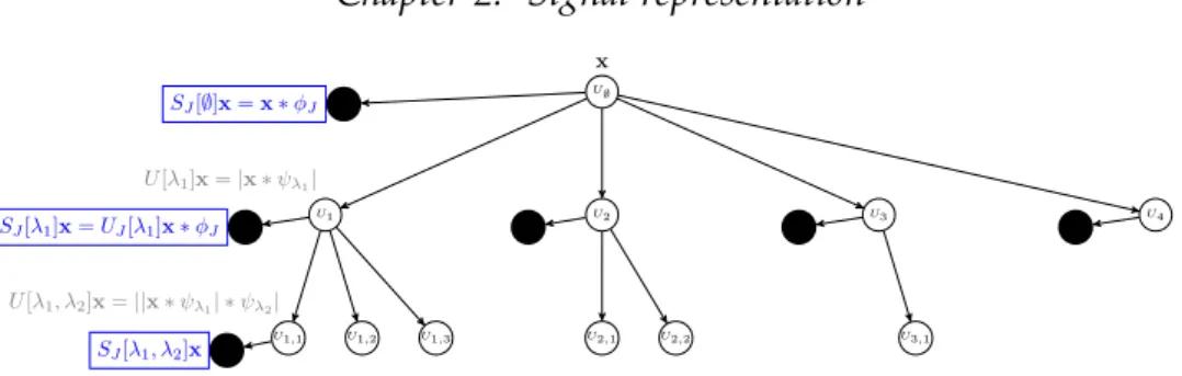
the path of length exactly m₋1. To construct that layer from the pre-vious ones, it is interesting to notice that for any given path p and an orientation-scale pair λ, we have U[λ]U[p] = U[p+λ]. We also remind that SJ[p](x)=d U[p]x∗φ₂J(u). So we can iteratively compute the nodes of the scattering network by first recursively computing the scattering prop-agators for all length m up to the pre-determined maximum depth of the network M. Then all the nodes value can be extracted by localising the scattering propagators with a scaled spatial window. Figure 2.7 provides a graphical representation of the scattering network.

In the end, the scattering network can be constructed by iteratively ap-plying a bank of filters and non linearity to an input signal. Thus creating an an architecture similar to a deep convolution network [98]. It has, how-ever, some particularities. Standard CNNs project the signal by applying a succession of convolution/pooling steps and extract the features used for inference at the final layer. The scattering network however outputs features at each layers (see Figure 2.7). Also, while convolutional neural networks use kernel filters learned from the data with back-propagation

algorithm, SCNs use a fixed wavelet filter bank.

It is interesting to take a closer look to the second layer of the SCN. The coefficients of the second layer are defined as{|x_∗ψλ| ∗φ2J(u)}. Using the DAISY approximation [104], one can recognise the SIFT coefficients [72], SJ[2jr] =|x∗ψ₂j_r| ∗φ₂J(u), whereψ₂j_r is the partial derivative of a Gaussian computed at the finest image scale 2j and for 8 different rotations r. The averaging filter φ₂J is a scaled Gaussian. So the second layer of the SCN is equivalent to the SIFT filters. The difference with them is in the fact that the information pipeline is iterated over to create more complex features.

U∅ x SJ[∅]x=x∗φJ U1 U[λ1]x=|x∗ψλ1| SJ[λ1]x=UJ[λ1]x∗φJ U1,1 U[λ1, λ2]x=||x∗ψλ1| ∗ψλ2| SJ[λ1, λ2]x U1,2 U1,3 U2 U3 1

Figure 2.7: A scattering propagatorUJ applied to a signalxcomputes each U[λi]x=|x∗ψλi|and outputsS[∅]x=x∗φ2J. ApplyingU_J to each

U[λi]xcomputes allU[λi,λj]xand outputsSj[λi] =U[λi]∗φ₂J. Applying iterativelyUJ to eachU[p]xoutputsSJ[p]x=U[p]x∗φ₂J

and computes the next path layer.

2.3.3

Properties of the scattering transform:

The scattering coefficient having been defined, one can be interested in the characteristics of such a data representation. This section provides an overview of some of the properties of the scattering transform. It also in-troduces an approximation to the scattering convolution network defined in the previous section, leading to computationally tractable networks.

2.3.4

Non-expansivity:

The path ordered scattering propagator_UJ[p]xresults of the composition of an unitary wavelet transformWJ with a non-expansive modulus operator —as_∀(a,b)_∈C2||a_{| − |}b_{|| ≤ |}a₋b_|— and is thus also non-expansive. Since the scattering transform SJ[PJ] iterates on UJ, one can prove that SJ[PJ] is also non-expansive (proof adapted from [46]).

Proposition 1. (Non-expansive)

The scattering transform is non expansive.

∀x,x0_{∈ L}2(Rd) _kSJ[PJ]x−SJ[PJ]x0k ≤ kx−x0k

2.3.5

Energy preservation:

Each scattering propagatorU[λ]x=|x∗ψλ|captures the frequency energy

contained in the signal x over a frequency band covered by the Fourier transform ˆψλ and propagates this energy towards lower frequencies. It can

thus be proved that under some assumptions on the wavelet —admissible wavelets—, the whole scattering energy ultimately reaches the minimum frequency 2−J and is trapped by the low-pass filter φ₂J. Thus the energy propagated by a —windowed— scattering transform goes to 0 as the path length increases, implying that _kSJ[PJ]k=kxk

But prior to showing this, one must states the necessary assumptions to be made on the wavelet used.

Note. The notation ˆ(.) is used to design the Fourier transform.

Definition 2.3.5. (Admissible scattering wavelet)

with|ρˆ(ω)| ≤ |φˆ(2ω)| andρˆ(ω) =0, such that the function, ˆ Ψ(ω) =|ρˆ(ω−η)|2− +∞

∑

∑

∑

For an admissible wavelet one can prove that the scattering transform conserves the energy of the signal.

Theorem 2.3.6. (Energy conservation)

If the scattering waveletψis admissible, then for all signalx∈ L2(Rd), lim m→+∞kU[Λ m J ]xk2=_mlim_→+∞ +∞

∑

The proof of the Theorem 2.3.6 also shows that the scattering en-ergy propagates progressively towards lower frequencies and that the energy of U[p]x is mainly concentrated along frequency decreasing paths p= (λk)k≤m, i.e. for which|λk+1| ≤ |λk|. The energy contained in the other paths is negligible and thus for the applications in this document only frequency decreasing paths are considered.

Moreover, the decay of∑+n=∞mkSJ[ΛnJ]xk2implies that there exist a path length M >0 after which all longer paths can be neglected. For signal processing applications, this decay appears to be exponential. And for

classification applications, paths of length M=3 provides the most inter-esting results [94, 106].

The restrictions stated above yield an easier parameterisation of a scat-tering network. Indeed when only the frequency decreasing paths up to a given order are considered, a scattering network is completely defined by:

• ψ: The admissible wavelet used. In the remainder of the document, unless stated otherwise, the Morlet wavelet is used.

• M: The maximum path length considered.

• J: The finest scale level considered.

• L: The number of orientation considered, which can be defined as the cardinality of the previously define ensembleG.

Hence for a given set of parameter (ψ,M,J,L), one can generate one and only one frequency decreasing paths scattering network. Let ST_(ψ,M,J,L)(x) now denotes the frequency decreasing windowed scattering convolutional network of parameter(ψ,M,J,L)evaluated for signalx. Each nodei of this network generates a -possibly empty- set of of nodes of size (ji−1)×L where ji is the scale of node i and L is the number of orienta-tions considered. Finally the number of nodesOof this network is,

O= M−1

∑

and it has the architecture displayed by Figure 2.8.

Translation invariance:

The translation invariance of the scattering transformSJ[PJ]can be proved for a limit metric when J goes to infinity. To do so one can first prove

U∅ x SJ[∅]x=x∗φJ U1 U[λ1]x=|x∗ψλ1| SJ[λ1]x=UJ[λ1]x∗φJ U1,1 U[λ1, λ2]x=||x∗ψλ1| ∗ψλ2| SJ[λ1, λ2]x U1,2 U1,3 U2 U2,1 U2,2 U3 U3,1 U4 1

Figure 2.8: Frequency decreasing scattering convolution network with J=4 scales, L=1 orientation and M=2 layers. A nodeiat scale ji

generates(ji−1)×Lnodes.

that the scattering distance kSJ[PJ]x−SJ[PJ]x0k converges when J goes to infinity — as it is non-increasing when J increases (see Section 2.3.4). From there one can bound the distance between the scattering transform of the signal and the one of its translated version kSJ[PJ]Lcx−SJ[PJ]xk and prove that this bound tends to 0 when J goes to infinity. This proves the translation invariance.

Theorem 2.3.7. (Translation invariance) For admissible scattering wavelets,

∀x_{∈ L}2(Rd), ∀c_∈Rd lim

J→∞kSJ[PJ]Lcx−SJ[PJ]xk=0

Lipschitz continuity to the action of diffeomorphisms:

The Lipschitz continuity to the action of diffeomorphisms of Rd can be proved for deformations sufficiently close to translations. Such diffeo-morphisms map u to u₋τ(u) where τ(u) is a displacement field such that k∇τk∞ < 1 —i.e. invertible transformations [121]. Let Lτx(u) =

x(u₋τ(u)) denotes the action of such diffeomorphisms on the signal x. Once again, one can find an upper bound to the distance between the scattering transform of the signal and the one of its deformed version

kSJ[PJ]Lτx−SJ[PJ]xk. With a bit of work on this bound, one can then

transla-tion term proportransla-tional to 2−Jkτk∞ and a deformation error proportional

to _k∇τk∞. Finally some more work on the bounding term provides the

Lipschitz continuity.

Theorem 2.3.8. (Lipschitz continuity to the action of diffeomorphisms) There exists C such that allx_{∈ L}(Rd)with_kU[_PJ]xk1<∞and allτ ∈ C2(Rd)

withk∇τk∞< 12 satisfy, kSJ[PJ]Lτx−SJ[PJ]x+τ.∇SJ[PJ]xk ≤CkU[PJ]xk1K(τ), (2.6) with K(τ) =2−2Jkτk2_∞+k∇τk∞ max log k∆τk∞ k∇τk∞, 1 +_kHτk∞.

Remark. If the case where 2J kτk∞ and k∇τk∞+kHτk∞1, thenK(τ) becomes negligible and the displacement field τ(u) can be estimated at each u∈ Rd. This can be done by solving the linear equation resulting from Equation 2.6 under the assumptions mentioned above,

∀p∈ PJkSJ[p]Lτx−SJ[p]x+τ.∇SJ[p]xk ≈0.

This estimate of the displacement field can be used for many applica-tions such as object tracking in video sequences or image sequence restora-tion [35].

2.3.6

Extensions

In the previous sections we have introduced a signal projection operator with local translation invariance, stability to deformations and yet still expressive. Building upon that basic architecture of wavelet filter fol-lowed by a non linearity, extensions of the scattering transform with extra properties have been developed. The results in Chapter Chapter 6 and

Chapter Chapter 7 can be, with little extra work, extended to those more complex transforms.

Sifre and Mallat [130] develop an extension to the scattering network offering partial rotation invariance to the projection operator. This extra invariance offers more robustness for natural image classification. Oyallon and Mallat [142] further improve and develop that concept.

Singh and Kingsbury [164] develop the scatternet. They follow the same general architecture of wavelet transform/non linearity, but use a parametric log transformation with Dual-Tree complex wavelets (DTCW) [76]. Leveraging the invertibility of the DTCW, they design a in-vertible projection.

2.3.7

Application to classification:

The scattering transform maps a given realisation of a high-dimensional signal into an even higher-dimensional space where the classification task is simplified due to the inherent properties described in the previous sec-tion yielding easily separable data clusters in the “scattering” space.

The scattering transform has been successfully applied in classifica-tion of a wild variety of signals such as audio signals [106], images [142] or electrocardiograms [135] and in the vast majority —if not all— the classi-fication task has been done using the features generated by the transform of the dataset as inputs for a discriminative classifier, e.g. Support Vector Machine classifier. The new input vector is obtained by concatenating the scattering coefficients of all orders, scale and orientations into a unique 1-D vector -for 2-D signal the scattering coefficients are also flattened. Lever-aging the richness of the representation generated the scattering transform combined to an SVM classifier provides performance comparable to those of a -small- deep convolutional neural network [129]. This section proposes

to test this framework on the handwritten digit datasetMNIST[151].

MNIST is composed of 28_×28 binary and centered images of hand-written digits. The dataset is split into a training set of 50000 images and a testing set of 10000 images and the task at hand is a 10 classes classification problem.

Figure 2.9: Samples from the MNIST handwritten digits recognition dataset.

For this task the frequency decreasing scattering convolutional net-work has M=3 layers, breaking down the images into J =3 scales and L=6 orientations. For each input image this networks generates 127 scat-tering coefficients (see Equation 2.5) and thus yields a 99568 dimensional feature vector (Number of scattering coefficients × image dimensions — i.e. 127_×28_×28). The discriminative classifier used is a set of binary SVM classifiers with a Gaussian radial basis function kernel [41]. This classifier have two meta-parameters. γ defines how influential a single training ex-ample is andCthe trade off between misclassification of training examples and simplicity of the decision surface. Those meta-parameters are fine-tuned by cross-validation toC=3 andγ=0.0018.

Using this set-up, the trained model scores 99.47% accuracy on the test set, i.e. 9947 true positive out of 10000 realisations. This accuracy is of the same order of what can be obtained using a convolutional neural network [90, 151]. For reference, when apply directly to the raw pixel a

linear classifiers reachs near 88% accuracy [45]. The improvement provided by the scattering network projection is a compeling argument for the need of signal representation prior to inference.

This approach of classification have been used successfully for many more applications but unfortunately it does not directly leverage the struc-ture created by the scattering transform and the possible information con-tained into it. Nor that it provides a generative models of the data, with all the advantages encompassed (see Chapter 3). In Part IV, we focus on building a generative model describing a scattering convolutional network.

Probabilistic Graphical Models

Probabilistic Graphical Models (PGMs) offer an efficient framework to ex-press joint distributions and conditional independencies. They rely on the usage of a graph based representation of conditional dependence between a set of random variables. Such graphs can then be used to encode a complete distribution over a multi-dimensional space in a compact —or factorised— manner. Probabilistic graphical models exist under many forms but they can be split into two main families, the Bayesian Networks (BNs) and the Markov models (MMs). Both families encompass the prop-erties of factorisation and independence defined by the graph, but differ when it comes to the specificities of the set of independence they can en-code as well as the factorisation of the distribution that they can induce [77].

In Part IV, we will use a probabilistic graphical model to describe the scattering network defined in Section 2.3.2. This chapter aims at providing the necessary prior knowledge for this work. Note, however, that we do not aim here at providing a complete overview of the probabilistic graph-ical models field but rather at introducing some concepts that are used in the remainder of this document. A reader further interested PGMs could refer to Heckerman [44], [91] or Bishop [77] for a more complete introduc-tion to those models.

models. Section 3.1 focuses on Bayesian networks, while Section 3.2 pro-vides more details about Markov models. Finally Section 3.3 introduces the basics of the approximate inference method known as variational inference.

3.1

Bayesian Networks:

A BN is subclass of probabilistic graphical model where the set of random variables and their conditional dependencies are expressed via a Directed Acyclic Graph (DAG). Those models can be used to describe either con-tinuous or discrete random variables as well as system governed by a mix of those. The architecture of Bayesian Networks is further explained in Section 3.1.1. Section 3.1.2 describes the inference mechanism for those networks and Section 3.1.3 presents a brief overview of the learning mech-anisms for BNs.

3.1.1

Architecture:

A BN is a graphical model encoding a joint probability distribution via a DAG.

Definition 3.1.1. Bayesian Network

For a set of random variables R={Ri}i∈J1,NK, a Bayesian network consists of a

direct acyclic graphG encoding a set of conditional independence assertions about the random variables in R and a setP of local probability distribution associated with each variable.

Each node of G encodes one of the random variable Ri and each edge Ei→j

represents the possible conditional dependence between nodes Ri and Rj.

Such networks encodes the conditional independence properties of the distribution [47].

Proposition 2. (Conditional independence for Bayesian networks)

nondescen-R

R

R

R

R

R

1

Figure 3.1: A simple Bayesian network.

dants in the graph given the value of all its parents.

P(_{Ri}i∈J1,NK) =

N

∏

P(Ri|Rρ(i))

where R_ρ(i) are the parents of the node Ri.

As a direct consequence to Property 2, one can say that a node with no parents is not conditioned on any other random variable considered. It defines a prior probability.

Property 2 allows to simplify the computation of the joint probability distribution represented by a Bayesian network. For example, for the net-work defined in Figure 3.1, the joint distribution can be obtained using the chain rule and theory on conditional independece,

P(R1,R2,R3,R4,R5,R6)

=P(R6|R3,R4,R5)P(R1,R2,R3,R4,R5)

=P(R6|R3,R4,R5)P(R3|R1,R5)P(R4|R2)P(R5|R2)P(R1,R2)

=P(R6|R3,R4,R5)P(R3|R1,R5)P(R4|R2)P(R5|R2)P(R2|R1)P(R1).

This example shows how BNs offer a convenient way to encode inde-pendence and an intuitive way to decompose the joint distributions.

3.1.2

Inference:

A Bayesian network encodes the full joint distribution of the studied ran-dom variables. This knowledge can be used to perform several interesting inference tasks among which are:

• Belief updating: Given some evidences —i.e. values for some nodes of the network_{Rj}j∈J whereJ is a subset of the graph— we compute the probability associated with an unobserved variable,

R∗_i =P(Ri|{Rj}j∈J). (3.1)

Ri such that the probability from Equation 3.1 is maximised defines a prediction for this node. This is one of the advantages of belief updating over other prediction methods, it can provide a probabilis-tic prediction even when given incomplete observations —i.e. a set

{Rj}j∈J such that J∪ {i} 6=R. Belief updating can be extended to the prediction of a set of unobserved variables.

• Optimal decision: A probabilistic graphical model can be used to express actions taken by an agent to modify the state of an uncertain

world. In this case given some evidence {Rj}j∈J where J is a subset of the graph _G one is interested in finding the set of action _{Ai}i∈A

where A is the set of all possible actions. To do so one also needs a reward function Oi(Ai) expressing the outcome of the action Ai, maximising the probability of the outcome ,

{A∗_i}i∈A=argmax A

P(_{Oi(Ai)}i∈A|{Ai}i∈A,{Rj}j∈J).

This type of inference is useful in Reinforcement learning framework where one is interested in learning the optimal set of actions to com-plete a task.

• Sensitivity analysis: Given some evidences —i.e. : values for some nodes of the network{Rj}j∈J where J is a subset of the graph— used for belief updating, one can be interested in assessing which among those random variables has the most influence on the prediction qual-ity. This means find,

∆∗

k =argmax k∈J

∆k

where ∆k defines the difference between the probabilities given the full set of evidences and given the set minus thek-th evidence,

∆k =P(Ri|{Rj}j∈J)−P(Ri|{Rj}j∈J\{k}).

This type of inference can be useful in the case where the evidence is expensive to collect, or when prediction has to be provided within a certain time. Then the sensitivity analysis allows to focus the effort into collecting/incorporating the most important piece of informa-tion.