Masthead Logo
Western Michigan University
ScholarWorks at WMU
Transportation Research Center Reports
Transportation Research Center for Livable
Communities
12-31-2015
14-08 Big Data Analytics to Aid Developing
Livable Communities
Li Yang
Western Michigan University, [email protected]
Hyunkeun Cho
Jun-Seok Oh
Western Michigan University, [email protected]
Follow this and additional works at:
https://scholarworks.wmich.edu/transportation-reports
Part of the
Transportation Engineering Commons
This Report is brought to you for free and open access by the
Transportation Research Center for Livable Communities at ScholarWorks at WMU. It has been accepted for inclusion in Transportation Research Center Reports by an authorized administrator of ScholarWorks at WMU. For more information, please [email protected].
Footer Logo
WMU ScholarWorks Citation
Yang, Li; Cho, Hyunkeun; and Oh, Jun-Seok, "14-08 Big Data Analytics to Aid Developing Livable Communities" (2015).
Transportation Research Center Reports. 32.
TRCLC 14-08
December 31, 2015
Big Data Analytics to Aid Developing Livable
Communities
FINAL REPORT
Li Yang, Hyunkeun Cho, Jun-Seok Oh
Transportation Research Center
for Livable Communities
Technical Report Documentation Page 1. Report No.
TRCLC 14-08
2. Government Accession No.
N/A
3. Recipient’s Catalog No.
N/A
4. Title and Subtitle
Big Data Analytics to Aid Developing Livable Communities
5. Report Date
December 31, 2015
6. Performing Organization Code
N/A
7. Author(s)
Li Yang, Hyunkeun Cho, Jun-Seok Oh
8. Performing Org. Report No.
N/A
9. Performing Organization Name and Address
Western Michigan University 1903 West Michigan Avenue Kalamazoo, MI 49008
10. Work Unit No. (TRAIS)
N/A
11. Contract No.
TRCLC 14-08
12. Sponsoring Agency Name and Address
Transportation Research Center for Livable Communities (TRCLC)
1903 W. Michigan Ave., Kalamazoo, MI 49008-5316
13. Type of Report & Period Covered
Final Report
7/1/2014 - 12/31/2015
14. Sponsoring Agency Code
N/A
15. Supplementary Notes 16. Abstract
In transportation, ubiquitous deployment of low-cost sensors combined with powerful computer hardware and high-speed network makes big data available. USDOT defines big data research in transportation as a number of advanced techniques applied to the capture, management and analysis of very large and diverse volumes of data. Data in transportation are usually well organized into tables and are characterized by relatively low dimensionality and yet huge numbers of records. Therefore, big data research in transportation has unique challenges on how to effectively process huge amounts of data records and data streams. The purpose of this study is to conduct research on the problems caused by large data volume and data streams and to develop applications for data analysis in transportation. To process large number of records efficiently, we have proposed to aggregate the data at multiple resolutions and to explore the data at various resolutions to balance between accuracy and speed. Techniques and algorithms in statistical analysis and data visualization have been developed for efficient data analytics using multiresolution data aggregation. Results will be helpful in setting up a primitive stage towards a rigorous framework for general analytical processing of big data in transportation.
17. Key Words
Data aggregation, data analytics, visualization, regression, statistical analysis.
18. Distribution Statement
No restrictions. This document is available to the public through the Michigan Department of Transportation. 19. Security Classification - report Unclassified 20. Security Classification - page Unclassified 21. No. of Pages 17 22. Price N/A
Title of the Project
Disclaimer
The contents of this report reflect the views of the authors, who are solely responsible for the facts
and the accuracy of the information presented herein. This publication is disseminated under the
sponsorship of the U.S. Department of Transportation’s University Transportation Centers
Program, in the interest of information exchange. This report does not necessarily reflect the
official views or policies of the U.S. government, or the Transportation Research Center for
Livable Communities, who assume no liability for the contents or use thereof. This report does not
represent standards, specifications, or regulations.
Acknowledgments
This research was funded by the US Department of Transportation through the Transportation
Research Center for Livable Communities (TRCLC), a Tier 1 University Transportation Center.
TRCLC 14-08
Big Data Analytics to Aid Developing Livable
Communities
Project Report
Li Yang, Hyunkeun Cho, Jun-Seok Oh
1
Introduction
In transportation, ubiquitous deployment of low-cost sensors combined with powerful computer hardware and high-speed communication network makes big data available. Big data are obtained from multiple sources including traffic sensors and sensor networks, video cameras, probe vehicles, travelers with mobile devices, transit and freight agencies, social networks, and software logs. Amounts of the obtained data are often beyond capacities of traditional data processing software. Technical challenges exist in storage, search, analysis, visualization, and exploration of these data. For data analytics, big data offers technical challenges in three major directions: high volume (amount of data), high velocity (speed of data flow), and high variety (various data structures, formats and sources). A big data set is so large that, for numeric processing, it cannot be loaded entirely into main memory for processing and, for data query and search, it is difficult to process using relational database and traditional data processing applications. As for data velocity, traffic sensors and sensor networks produce endless data streams demanding for real-time processing. Processing of these data must work “on-the-fly” and has only one chance to look at the data. As for variety of data types and sources, big data analytics requires multimodal processing and
integration of large data sets from various sources. Clearly, these problems pose fundamental
challenges by changing our assumptions of traditional data. Big data analytics requires new forms of processing to enable enhanced decision making, insight discovery and process optimization.
Unlike big data with high dimensionalities and/or complex structures in many areas, big data in transportation are usually organized into relational tables and are characterized by relatively low dimensionality and huge numbers of records. Therefore, big data research in transportation has its unique challenges and opportunities. A major challenge is how to process huge amounts of data records and data streams effectively and efficiently.
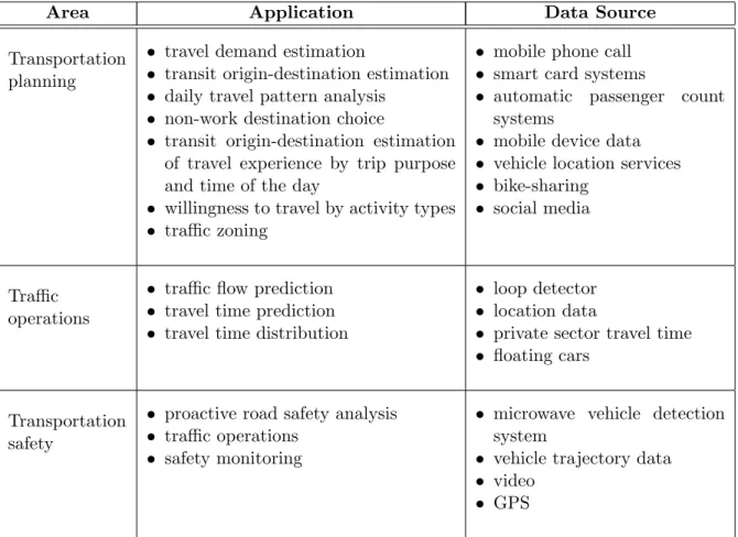
USDOT defines big data research in transportation as a number of advanced techniques applied to the capture, management and analysis of very large and diverse volumes of data. Analysis of these data at fine granularity offers opportunities to integrate intelligence not only into transportation infrastructure but also drivers, multimodal travelers and freight carriers with huge benefits. These benefits include increased accuracy of prediction, improved operation insights, and new travel products and services. Big data analytics help to answer key questions, such as how to predict and mitigate traffic congestion, how to reduce traffic crashes and improve road safety, how to analyze and optimize individual travelers’ trip planning, how to maximize utilization of existing transportation infrastructure, how to coordinate multimodal transportation systems and networks, how to reduce supply chain waste by optimizing freight movements, etc. Table 1 briefly lists areas
Area Application Data Source
Transportation planning
• travel demand estimation
• transit origin-destination estimation
• daily travel pattern analysis
• non-work destination choice
• transit origin-destination estimation
of travel experience by trip purpose and time of the day
• willingness to travel by activity types
• traffic zoning
• mobile phone call
• smart card systems
• automatic passenger count
systems
• mobile device data
• vehicle location services
• bike-sharing
• social media
Traffic operations
• traffic flow prediction
• travel time prediction
• travel time distribution
• loop detector
• location data
• private sector travel time
• floating cars
Transportation safety
• proactive road safety analysis
• traffic operations
• safety monitoring
• microwave vehicle detection
system
• vehicle trajectory data
• video
• GPS
Table 1: Big data in transportation: Areas, applications, and example data sources.
in transportation using big data, typical applications in each area, and example data sources used.
2
Project Overview
Big data analytics becomes an upcoming movement in transportation research. Technical chal-lenges are extreme and force us to rethink data processing algorithms, techniques and systems in fundamental ways. As a pilot study, this project was proposed to focus on these challenges, especially the problems caused by large data volume and data streams, and develop real-world applications for transportation data analysis.
In analysis of large amount of data records, the most significant problem comes from the conflict between the requirement of accessing a data set in its entirety and the reality that the data is stored record by record. Relational database systems are traditionally optimized to efficiently access individual data records. This conflicts with data access pattern of data analytics where global access of the entire data set is the most frequent data operation. These observations suggest that large data in their raw format are rarely appropriate for data analysis. A key challenge is to create data representations and transformations that convert a large amount of data into forms that facilitate global access and analytical understanding.
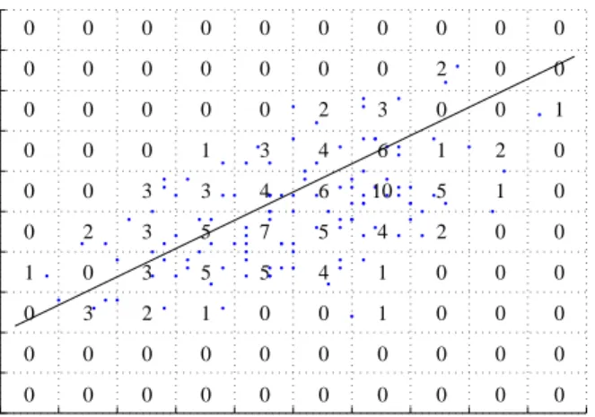
One efficient way to reduce data size is to aggregate data. We illustrate the main idea in this project using Figure 1, where the data space is partitioned into small cells and the value in each cell represents the number of data records in the cell. A linear regression model can be learned from
0 0 0 0 0 0 0 0 0 0 0 0 0 0 0 0 0 0 0 0 0 3 2 1 0 0 1 0 0 0 1 0 3 5 5 4 1 0 0 0 0 2 3 5 7 5 4 2 0 0 0 0 3 3 4 6 10 5 1 0 0 0 0 1 3 4 6 1 2 0 0 0 0 0 0 2 3 0 0 1 0 0 0 0 0 0 0 2 0 0 0 0 0 0 0 0 0 0 0 0
Figure 1: Linear regression from aggregated data instead of individual records.
positions of the cell centers and the associated count values by assuming all data points in each cell locate at the center of the cell. The learned model is close to the model that would be directly learned from individual data points. To refine the model, we can further partition each cell into smaller cells and, therefore, organize the aggregated data hierarchically at multiple resolutions. An algorithm may start to access aggregated data at a coarse resolutions and then selectively get data at finer resolutions if deemed necessary. In this way, resolution serves as a extra control and offers a compromise between speed and accuracy in data analysis.
The objective of this project is to conduct fundamental research of working with aggregated data and to develop techniques and tools for big data analytics in transportation. To process large number of data records efficiently, we have proposed to aggregate data at multiple resolutions and to explore the data at various resolutions to balance between accuracy and speed. Based on our previous work on large data visualization using multiresolution data aggregation as an intermediate data representation, we have studied techniques and algorithms for efficient data analytics in transportation. Specifically, we have transformed about six terabytes of NAVTEQ Real-Time Flow Feed data for major Michigan roadways and imported them to a MySQL database to provide a common platform to facilitate data analysis. It includes a database, the corresponding web services to answer user queries, and utility functions to collect, integrate, extract and store data from real-time data streams. We have applied statistics models to transportation data and have conducted clustering and regression analysis using multiresolution data aggregates as data input. We have studied multidimensional visualization of traffic data using parallel coordinates and have explored data cubing operation and interactive visual exploration of iceberg data cubes for visual data mining. These activities are further described in the rest of this report.
3
Data Transformation, Loading, and Preprocessing
As a step for data preprocessing, we have developed ETL (Extraction, Transformation and Load-ing) tools to import archived and real-time NAVTEQ Real-Time Flow Feed data to a MySQL database. The feed data is given in TrafficML format, which is a special XML format for traffic data specification. Figure 2 shows a sample data record in the TrafficML data format.
<?xml version="1.0" encoding="UTF-8" standalone="yes"?> <TRAFFICML_REALTIME xmlns="trafficml50_realtime" VERSION="5.0" TIMESTAMP="12/30/2012 04:36:58 GMT" NAVTEQ_VERSION="201101"> <ROADWAY_FLOW_ITEMS> <ROADWAY_FLOW_ITEM> <ROADWAY_ID>108+00067</ROADWAY_ID> <DESCRIPTION>I-96</DESCRIPTION> <FLOW_ITEMS DIRECTION="+"> <FLOW_ITEM> <ID>108+04236</ID> <RDS_LINK> <LOCATION> <EBU_COUNTRY_CODE>1</EBU_COUNTRY_CODE> <TABLE_ID>8</TABLE_ID> <LOCATION_ID>04236</LOCATION_ID> <LOCATION_DESC>I-75</LOCATION_DESC> <RDS_DIRECTION>-</RDS_DIRECTION> </LOCATION> <LENGTH UNITS="mi">1.24575</LENGTH> </RDS_LINK> <CURRENT_FLOW> <TRAVEL_TIMES> <LANE_TYPE TYPE="THRU"> <TRAVEL_TIME TYPE="current"> <DURATION UNITS="min">1.26</DURATION> <AVERAGE_SPEED UNITS="mph">67.57</AVERAGE_SPEED> </TRAVEL_TIME> <TRAVEL_TIME TYPE="freeflow"> <DURATION UNITS="min">1.26</DURATION> <AVERAGE_SPEED UNITS="mph">59.20</AVERAGE_SPEED> </TRAVEL_TIME> </LANE_TYPE> </TRAVEL_TIMES> <JAM_FACTOR>0</JAM_FACTOR> <JAM_FACTOR_TREND>0</JAM_FACTOR_TREND> <CONFIDENCE>0.92</CONFIDENCE> </CURRENT_FLOW> ...
Figure 2: Sample data records in TrafficML format.
on major Michigan roadways for 10 years up to the year of 2012. There are over 6000 package files which contains about 3 million XML files. After decompression, the total size of the XML files is about 6 TBytes. The data set has a total number of more than 2 billion records.
Our task was to import the data into a MySQL database running on a Dell Precision workstation with an Intel Xeon processor and 32GB of memory. To improve performance of disk I/O, we have set up a disk array of multiple hard disks. The built-in XML data importing utility in MySQL database does not navigate through XML tags and cannot parse the above XML correctly. We thus wrote XSLT (eXtensible Stylesheet Language Transformations) stylesheets and used a XSLT processor to transform the XML data to a text file and then import the text file to the MySQL database. The loading of the entire data set to database took about 24 hours.
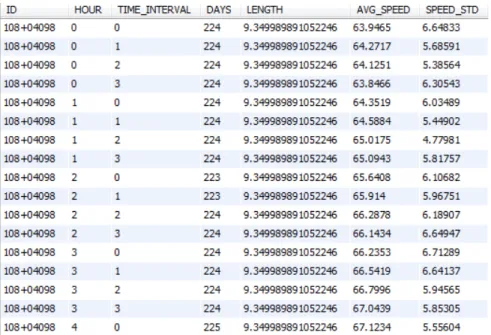
NAVTEQ Real-Time Flow Feed data report average traffic speeds with time intervals of a few minutes on each road segment. Once the data are loaded into database, we can use database query to answer questions and perform processing tasks. To remove outliers, for example, one possible way is to calculate the average traffic speed at each particular time of the day on each road segment for one month. Traffic speed records in the month are then compared with the corresponding average traffic speed of the month. If a record has traffic speed much bigger or smaller than the monthly average speed, the record will be treated as outlier. With the outliers eliminated, we can aggregate the speed data according to various time slots and locations. Figure 3 shows the beginning of a
Figure 3: Data aggregation query (ID: road segment ID, HOUR (0-23): hour in a day, TIME INTERVAL (0-3): quarter in an hour, DAYS: valid number of days in a year, LENGTH: length of road segment, AVG SPEED: average of traffic speeds, SPEED STD: Standard derivation of speeds)
table of average speeds at quarter hour intervals on road segments.
Many useful data analysis functions can be implemented as SQL database queries. Using Michi-gan traffic accident database as a reference, for example, we can pick up traffic speed information at the time and location of accidents for better understanding of traffic behaviors during accidents. We have written a client program to connect to the MySQL database. The client program can find average speeds at times of accidents as well as speeds of both upstream traffic and downstream traf-fic at the accident spot. The query results can be used as input data to graphing and visualization applications that can help users better understand the data.
4
Clustering and Regression Analysis Using Multiresolution Data
Aggregation
Data clustering and regression analysis are basic functions in statistical data analysis. Analysis of massive data is challenging due to size limitations of computer memory and the maximum array size in software environments. Moreover, computation may take a long time if the underlying algorithm has high complexity. Using large data sets, we can hardly load the entire data into main memory. Thus we have to develop efficient techniques to support the processing of data with large size.
In recent years, the divide and conquer regression approach has been studied [2, 4, 11, 12]. This approach partitions a large data set into subsets, analyzes each set separately, and combines the analyses intelligently. Although the above methodologies can reduce the required amount of primary memory, they are not directly applicable for analyzing multiresolution aggregated data. The multiresolution data aggregation requires new statistical paradigm since it has to work with aggregated data rather than individual data records.
two-dimensional data set where each data record is a pair (X, Y) as shown in Figure 1. Suppose that the data set is big such that traditional statistical approaches utilizing the entire data are not feasible, we consider a different approach using aggregate data to analyze the marginal regression
mean model Y =β0+β1X+. We partition the coordinate plane into cells and consider a set S
of non-empty cells each with at least one data record. Instead of storing the original data set, we
keep the center (Xc, Yc) of each cell in S and the number of data records in the cell. This is the
aggregated data, the size of which is much smaller than the size of the original data.
Another way of data aggregation is to replace the center (Xc, Yc) with results of cluster analysis,
which is to partition the data records by assigning similar records into the same cluster. For cluster
analysis, one method is the k-means method which partitions data records into k initial clusters
by assigning a data record to the cluster whose centroid is nearest, recalculate the centroid for new data clusters and do assign data records again until no data record changes clusters. Another clustering method is hierarchical cluster analysis that starts with each data record as a cluster,
computes the distances between clusters, then merges nearest clusters, and repeats until we get k
clusters.
From the aggregated data, regression analysis can be easily implemented using the center or cluster of data as input data with weights depending on the number of data records in each cell or cluster. This approach is quite challenging in asymptotic theory, yet holds consistency and normality as the cell size goes to infinity. In this project, the choice of cell size has been investigated since it plays an important role in parameter estimation. Our approach obtains precise estimates without analyzing the entire data set. By choosing the proper size of cells, we can balance between efficiency and accuracy of estimation.
5
Analysis of Multivariate Longitudinal Data Using Multivariate
Marginal Models
Big data are often archived over a long period of time. Therefore multivariate longitudinal analysis has gained increase in popularity. In transportation studies, subjects are often measured on multiple times with regard to a collection of response variables. In transportation safety studies, for example, various records such as the number of crashes, presence of fatal crashes, rate of incapacitating injury crashes in addition to identifying the crash modification factors are repeatedly measured on many intersections or roads.
Multivariate longitudinal data provides a unique opportunity in studying the joint evolution of various responses over a period of time. The analysis of multivariate longitudinal data can be challenging because repeated measurements from the same roads and different response variables within the same location are likely to be correlated. In this study, we develop multivariate marginal models in longitudinal studies with multiple response variables, and improve parameter estimation by incorporating informative correlation structures. This work has been reported in [1].
Suppose yi·k = (yi1k, . . . ,yiJik)
0 is the kth response variable measured J
i times from the ith
subject, andyijk’s are independent identically distributed for i= 1, . . . , N, where N is the sample
size and Ji is the cluster size. To simplify the notation, we set Ji = J for all subjects. For the
generalized linear model, the formulation of multivariate marginal models is defined as
µijk =E(yijk|xij) =µ(x0ijβk), (1)
whereµ(·) is an inverse link function,βk= (βk1, . . . , βkP)0 is aP-dimensional parameter vector for
To accommodate the association between responses, we stack up the response variable asYi= (yi0·1, . . . ,y0i·K)0 and Xi = (IK ⊗xi) is extended to a P K ×J K matrix by Kronecker product
operator, whereK is the number of responses,xi= (xi1, . . . ,xiJ) is aP×J matrix,IK is aK×K
identity matrix and⊗corresponds to a left Kronecker product. The corresponding parameter is a
P K-dimensional vector ofβ= (β01, . . . ,β0K)0 and the marginal model in (1) is represented asµi=
E(Yi|Xi) = µ(X0iβ). We extend the quasi-likelihood to incorporate the correlation information
and obtain the estimator by solving N
X
i=1
˙
µ0iA−i 1/2R(α)−1A−i 1/2(Yi−µi) = 0, (2)
where ˙µi = (∂µi/∂β), Ai is the J K×J K diagonal marginal variance matrix of Yi, and R(α)
is the working correlation matrix that contains correlation parameters α. The approach requires
only a few nuisance parameters α to specify a common working correlation structure such as an
exchangeable or the first-order auto-regressive correlation.
For the multivariate marginal model, the working correlation structure R(α) enables us to
accommodate three pieces of association information; the correlation across time within the subject, the cross-correlation between different response variables both at the same time and across time. Therefore, the simple working correlation structure such as exchangeable or the first-order auto-regressive does not represent the true correlation structure sufficiently. It is well-known that when the correlation structure is incorrectly specified, the estimator can be inefficient. If the unspecified
correlation structure is considered as the working correlation matrixR(α), there are (J K)×(J K−
1)/2 correlation parametersα to be estimated, which might cause convergence problems when the
cluster size is large.
To avoid the estimation of α, the inverse of R is formulated by a linear combination of basis
matrices, R−1 =b0I+ q X m=1 bmBm, (3)
where I is an identity matrix, B1, . . . ,Bq are basis matrices with 0 and 1 components and bm’s
are unknown coefficients. By replacingR(α)−1 in (2) with basis matrices in (3), we introduce the
following score vector
GN(β) = 1 N N X i=1 gi(β) = 1 N PN i=1µ˙ 0 iA −1 i (Yi−µi) PN i=1µ˙ 0 iA −1/2 i B1A −1/2 i (Yi−µi) .. . PN i=1µ˙0iA −1/2 i BqA −1/2 i (Yi−µi) . (4)
Note that the estimating equation (2) is a linear combination of elements of the score vector (4) and
GN(β) does not involve nuisance parametersb0, . . . , bm. In addition, it follows from the moment
assumption E(Yi) = µi in (1) that E{gi(β)} = 0 under the true parameter. However, we cannot
set each component in (4) to zero in estimating β, since the dimensionality of GN(β) is greater
than the number of parameters. Instead, the estimating equations in (4) can be optimally combined
using the generalized method of moments. The idea is to construct an estimator of β by setting
specified linear combinations of GN(β) in (4) as close to zero as possible. That is, estimator ˆβ is
obtained by minimizing
where CN(β) = N1 PNi=1gi(β)gi(β)0 is a weighting matrix that estimates the covariance matrix
of gi(β) consistently. The function QN(β) optimally combines the estimating equations in (4)
and improves the efficiency of parameter estimation by representing the correlation structure as pre-specified basis matrices in (3). The proposed method yields a consistent and efficient estimator which follows an asymptotic normal distribution. Moreover, the proposed multivariate model en-ables us to estimate all parameters corresponding to multiple responses simultaneously even if the outcomes belong to different response families such as continuous, discrete and categorical variables. The multivariate modeling approach is applied on a real longitudinal data set in the transporta-tion safety study. The data consist of midblock segments of arterial roads in Lincoln, Nebraska between 2003 and 2007. In order to assess the impact on the safety of the arterial roads, the crash frequency (Crash) and the indicator variable showing presence of crash severity (Severe) were fol-lowed up annually and considered as response variables. Note that the two response variables are correlated because the crash severity can be observed only when the crash happens. Six covariates were also measured using Google Earth: The number of through lanes in the mid-block segment (Lane), average annual daily traffic per through lane (AADT), presence of median (Med), central business district (CBD), and length of mid-block segment (Segment). According to types of re-sponse families, two generalized linear models, Poisson and logistic regressions with log and logit link functions respectively, are formulated as
log{E(Crash)} = α0+α1Lane +α2AADT +α3Med +α4CBD +α5Segment,
logit{E(Severe)} = β0+β1Lane +β2AADT +β3Med +β4CBD +β5Segment.
To provide more accurate prediction models by accommodating correlation information, we
estimate all α’s and β’s simultaneously through the proposed method, and compare them with
the estimators based on the univariate marginal models utilizing the quadratic inference function and the generalized estimating equation. Here the first-order auto-regressive working correlation structure for estimation is utilized, since measurements within the same segment are less likely to be correlated if they are further apart in time. For the Crash log-link model, the coefficients of AADT and Segment are all positive with the corresponding small p-values less than 0.001, implying that the number of crashes would increase with average annual daily traffic per through lane and length of mid-block segment. Contrary to the Crash response, the result shows that the median might reduce the probability of crash severity significantly. Moreover, the chance of crash severity in central business district is lower than in other locations. Overall, the estimators obtained by the proposed method are sensible compared to other approaches for the two different types of generalized linear models.
For transportation safety studies, it is of particular interest to find relevant factors with regard to multiple response variables. In other words, one is interested in testing a hypothesis about a
subset of the β’s. We first decompose the regression parameter into two sets β = (θ,ϑ), where
θ is a regression parameter of interest with dimension S and ϑ is the nuisance parameters with
dimensionP K−S. The hypothesis is defined as
H0:θ=θ0 versus HA:θ6=θ0, (6)
whereθ0is a constant vector. As a special case, we can test a regression parameterβkcorresponding
to the kth response for k= 1, . . . , K; e.g., θ =βk and ϑ contains all regression parameters in β,
butβk.
We propose the test statistic for the hypothesis in (6) based on multivariate marginal models.
Since the quadratic inference function plays a similar role as the least square function, QN(θ0,ϑ˜)
˜
ϑ= argminϑQN(θ0,ϑ) and (ˆθ,ϑˆ) = argmin(θ,ϑ)QN(θ,ϑ). Although QN(θ0,ϑ˜) is systematically
greater than QN(ˆθ,ϑˆ) under HA, the gap between QN(θ0,ϑ˜) and QN(ˆθ,ϑˆ) must be very small
underH0. Therefore, an appropriate test statistic that testsH0 againstHAis
Tχ=N{QN(θ0,ϑ˜)−QN(ˆθ,ϑˆ)}. (7)
The test statisticTχ asymptotically follows the chi-squared distribution withS degrees of freedom
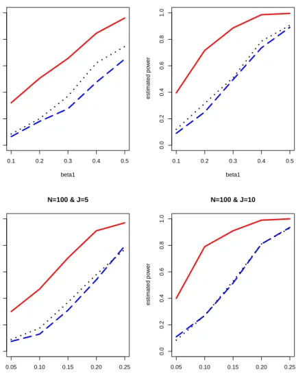
under the null hypothesis in (6) as N → ∞. In order to investigate how the power depends on
the magnitude of parameter, we estimate the power on β1 ∈[0.05,0.5]. We test H0 :β1 = 0 and
figure estimated power curves for N = 25,100 and J = 5,10 under the AR1 working correlation
structure. The exchangeable working correlation structure also has been applied, but the result is not reported because it is similar to Figure 4. The chi-squared test based multivariate marginal models is more powerful than the Wald-test under the univariate generalized estimating equation method (UGEE) and the chi-squared from the univariate quadratic inference approach (UQIF).
Specifically, whenβ1 is smaller than 0.1, the power of the proposed method is approximately three
times higher than those of the UGEE and UQIF approaches. As the parameter becomes a strong signal, the power of the proposed method approaches 1, while the powers of the UGEE and UQIF
are still lower than 0.9 whenβ1 = 0.5 andN = 25. In summary, the result in Figure 4 ensures that
the chi-squared test based on the proposed approach has stable and high power behavior.
6
Visual Data Exploration Using Multiresolution Data
Aggrega-tion
In addition to statistical data analysis, data visualization and exploration are areas where big data raise fundamental challenges. For visualization of large data sets, the basic assumption of loading the entire data set into memory and processing in memory is no longer valid, yet users have the same demand for interactivity and response time as they have for small data sets. Visualization techniques need to work closely with database. However, relational database systems are tradi-tionally optimized to efficiently access individual data records. This conflicts with the data access pattern of data visualization where browsing, zooming, and range query are the most frequent data operations. Efficient executions of these operations are beyond the capability of relational database systems.
In this project, we have applied a density-based data representation[9] to transportation data vi-sualization and exploration. To support the overview-and-drill-down data access pattern, relational data are aggregated into density representations and are organized in multiple resolutions. To or-ganize the data aggregated at multiple resolutions, we piggyback the aggregated data onto internal nodes of a high dimensional tree index. We have used a variation of the kdB-tree[6] data structure as an external high dimensional index to organize multiresolution data aggregations. Data required by visualization operations are then accessed by index-only queries that visit the aggregated data in internal nodes of the tree index. Two existing visualization techniques, footprint splatting and density-based parallel coordinates, are extended and integrated to accept aggregated data. Details of this research are presented in [8].
6.1 Multiresolution data aggregation
In order to resolve the conflict between user interaction with large relational data sets and the inability to scan the data in real time, we suggested to use a density representation[9] of data as an intermediate data interchange mechanism between database and visualization tools. The density
0.1 0.2 0.3 0.4 0.5 0.0 0.2 0.4 0.6 0.8 1.0 N=25 & J=5 beta1 estimated po w er 0.1 0.2 0.3 0.4 0.5 0.0 0.2 0.4 0.6 0.8 1.0 N=25 & J=10 beta1 estimated po w er 0.05 0.10 0.15 0.20 0.25 0.0 0.2 0.4 0.6 0.8 1.0 N=100 & J=5 beta1 estimated po w er 0.05 0.10 0.15 0.20 0.25 0.0 0.2 0.4 0.6 0.8 1.0 N=100 & J=10 beta1 estimated po w er
Figure 4: Estimated power curves of chi-squared tests using the proposed approach (solid curve), UQIF (dashed curve), and Wald-test of UGEE (dotted curve).
representation of data has many important advantages. One obvious advantage is that it has a much smaller size than the original relational data. The number of records in the density data depends more on resolution than on the number of records in the original data. This makes data visualization scalable to the size of the original data. Furthermore, many density areas are thin, representing fewer original data records than a predefined threshold. Depending on which technique is used to visualize the data, those thin areas could be ignored because they hardly contribute any noticeable visual effect to the final visualization.
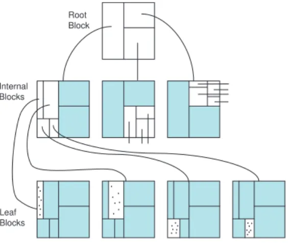
To facilitate overview-and-drill-down, density data representation should be available at multiple resolutions. We have found that a partition-based high dimensional tree index offers an excellent vehicle to organize the data aggregated at multiple resolutions, provided that the data have been aggregated according to the regions represented by internal nodes of the tree index. We have further found that major database problems (multiresolution data aggregation, optimization of range queries and other interaction-driven queries) in visual data exploration can be properly
Root Block Leaf Blocks Internal Blocks
Figure 5: An example 2dB-tree.
Hyper-rectangle ranges Internal node (dim,val) Leaf node (ptr, aggre_vals) Leaf node (ptr, aggre_vals) Leaf node (ptr, aggre_vals) Internal node (dim,val)
Figure 6: An internal block of data aggregation tree.
answered by index-only queries on such an index structure. We call the tree index adata aggregation
tree.
We have chosen to implement data aggregation tree using the basic kdB-tree[6] as our primary data access method for its simplicity and its direct extension of the kd-tree. Figure 5 illustrates
an example kdB-tree whenk is two. Each node of a kdB-tree represents a hyperrectangle in high
dimensional space and can be stored in a single hard disk block. Each non-leaf disk block contains a collection of block pointers, each of which points to another disk block, that partition the hyper-rectangle into smaller hyperhyper-rectangles. In order to piggyback the data aggregation information, we have revised the internal structure of kdB-tree blocks in data aggregation tree. Figure 6 gives the structure of non-leaf blocks in a data aggregation tree. Each non-leaf block contains a header and a body. The header defines the hyperrectangle represented by the block by recording the low and high values on each dimension of the hyperrectangle. The body encodes a binary kd-tree. Each non-leaf node of the kd-tree partitions the hyperrectangle it represents into two smaller hyperrect-angles represented by its two child nodes. The non-leaf node has the format of (dim, val) which records the partitioning dimension and the partitioning value. Data aggregation values are kept in leaf nodes of the kd-tree. Each leaf node represents a hyperrectangle and has the format of (ptr, aggregate-values), where ptr is a pointer pointing to a disk block of the data aggregation tree representing the hyperrectangle and aggregate-values represent a list of data aggregation values, such as count, sum, minimum, and maximum, of all data records within the hyperrectangle. The kd-tree nodes in a disk block are stored in a pre-order format. This helps to store more tree nodes in a disk block.
Hyperrectangle information in the header of each block can be computed in a top-down manner using the header and partitioning information contained in the parent block. Data aggregation values in a block can be computed in a bottom-up manner from the corresponding aggregation values in its direct child blocks. The user decides which aggregation values are stored when building the data aggregation tree.
when a block becomes full and a new entry is inserted, kdB-tree splits the block into two blocks in such a way that both contain similar numbers of child nodes. Such a split may cascade to the child nodes and cause the child nodes to split. We have modified the block splitting strategy of data aggregation tree for data insertion: (1) When a leaf block is full and has to split, it splits at the median value of all data records within the block along the longest dimension of the hyperrectangle it represents. Therefore, a leaf block splits into two leaf blocks with equal number of data records. (2) When a non-leaf block is full and has to split, it splits at the root node of the kd-tree it contains. In other words, it splits by following the first partition of the hyperrectangle represented by the block. This splitting strategy avoids cascading splits at the cost of creating a height unbalanced tree. The strategy keeps hyperrectangles in a data aggregation tree as hypercubic as possible, which helps us to explore data at a consistent resolution by visiting nodes at similar levels of the tree.
Browsing of data aggregation information is supported by visiting internal blocks at a given resolution of the data aggregation tree. There are multiple ways to define resolution. The simplest way is probably by the depth of the data aggregation tree. Data resolution can also be defined in ways more meaningful than tree depth. For example, resolution of a data hyperrectangle can be defined by its geometric measure (volume, range of the longest dimension) or by its data aggregate measure (number of data records, sum or maximum or minimum of values in a dimension). A
resolution measure associates a functionf(v) with each tree nodev. The only requirement is that
f(v) is anti-monotone to the depth of the tree, that is,f(vi)≥f(vj) ifvi is an ancestor node ofvj
in the tree. Given a particular resolution thresholdr, we define acut C(r) of the data aggregation
tree as
C(r) ={v|f(v)≤r∧f(parent(v))> r}.
C(r) can be intuitively thought as a horizontal cut across the data aggregation tree. In each
path from the root of the tree to a leaf, there is exactly one node included in C(r). The union of
hyperrectangles represented by all nodes inC(r) is the whole volume. The position ofC(r) changes
smoothly as the value of r changes. The larger r is, the closer the cut is to the root of the tree;
the smaller r is, the closer the cut is to the leaves of the tree. To browse aggregated data at the
resolution specified by r, we only need to access tree nodes in C(r). By changing the value of r,
we are able to explore a data set at different resolutions. Zooming and drill-down are supported
by changing the value of r. Because r is continuous, changing r will provide smooth transitions
in data exploration. This process may continue until leaf pages are accessed and individual data records are retrieved.
6.2 Visualizing Aggregated Data in Parallel Coordinates
Multiresolution data aggregation represents a new format of data for data visualization. An appli-cable visualization technique must be able to deal with high dimensionality, accept this new format of input data, and support user interactions such as zooming, picking, and brushing. We have chosen to extend parallel coordinates[3] as an example visualization technique to render multires-olution data aggregations. In addition to parallel coordinates, we also support 3D scatterplot and footprint splatting with animation supported by using grand tour.
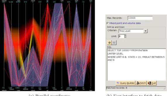
Figure 7 gives an example of visualizing aggregated data in parallel coordinates. Parallel co-ordinates horizontally arranges vertical coco-ordinates, one for each dimension. The original parallel coordinate visualization displays a data record as a polyline that crosses each coordinate at a posi-tion corresponding to its value on that dimension. The number of dimensions that can be visualized is restricted only by the horizontal resolution of computer display, although too many coordinates may make the visualization difficult to understand. We extended parallel coordinates to visualize data aggregations by displaying hyperrectangles in the data aggregation tree as horizontal opacity
(a) Parallel coordinates. (b) User interface to fetch data..
Figure 7: Density-based parallel coordinates and a user interface to specify resolution and SQL-style statements to fetch data.
bands. The location of a band across each coordinate reflects the position of the corresponding data hyperrectangle in that dimension. The extend of the band represents the span of the data hyperrectangle in that dimension. The opacity of each band is a function of the density of its cor-responding data hyperrectangle. The middle of each band is encoded with the deepest opacity. A band fades gradually from the dense middle to fully transparent edges. Bands of all hyperrectangles are blended to produce the final image.
This visualization allows a user to specify a horizontal data selection band (the gray band in Figure 7(a)). The data selection band represents a hyperrectangle as a query region in the data space. The data selection band can be used to issue a range query to the data aggregation tree for the purpose of data selection. This allows the user to visualize subsets of data in different levels of detail.
As discussed previously, data aggregation tree supports two types of user interactions: data se-lection with range query, and overview-and-drill-down by changing the resolution threshold. Range query criteria can be directly specified as a data selection band in the parallel coordinate visualiza-tion, as shown in Figure 7(a). Figure 7(b) shows a graphic user interface which contains a window through which the user can specify and change the resolution measure. The window also contains a text area which allow the user to give an SQL-style statement that specifies the query region as well as the resolution. Once the user clicks the “fetch” button, the statement will be sent to the server to get the aggregated data.
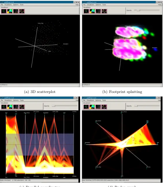
As an example, we have applied the visualization tool to the Fatality Analysis Reporting System (FARS) [5] data sets from the US National Highway Traffic Safety Administration. Accumulated from 1975, FARS has collected more than one million records on traffic accidents. We have selected 8 variables to visualize. Figure 8 gives screen snapshots showing different visualizations of this data set. Figure 8(a) gives a simple projection against three categorical variables: atmosphere, light condition, and surface type. The color represents Manner of Collision. Because each variable has only a few values, thousands of points are projected to the same position in the 3D scatterplot. The color of a position is the color of the last point drawn to that position. Occluded points are not
(a) 3D scatterplot (b) Footprint splatting
(c) Parallel coordinates (d) Radar graph
(a) Overview of data (b) Selected data visualized at higher resolution Figure 9: Screen snapshots of the 1% PUMS housing unit records.
shown at all. Figure 8(b) shows footprint splatting of the same projection. The data are visualized at predefined resolutions for continuous variables and against each individual value for categorial variables. Each data hyperrectangle is projected as a footprint whose opacity is determined by the number of data records in the hyperrectangle. Because the grand tour uses dynamic graphics, it is difficult to convey 3D rendering results through static screen snapshots. In our approach, a 3D feeling is obtained through animation. Sparse areas in the data can be seen by rotating the volume. It is clear from Figures 8(a) and 8(b) that volume rendering of aggregated data conveys density information while its scatterplot counterpart is overplotted. Figure 8(c) visualizes the data in parallel coordinates, where a gray data selection band runs across all coordinates at default positions. The data selection band specifies a query region which can be used to retrieve a subset of the data. When the user moves the cursor to a displayed coordinate, the corresponding range of values of the data selection band is displayed in footnote. Figure 8(d) visualizes the data in a radar graph which is a variation of parallel coordinates.
As another example, we have used this approach to visually explore the 1% Public Use Microdata Sample files (known as 1% PUMS) [7] made public by the US Census 2000. The data set contains both housing unit records and a number of person records for surveyed people living in each housing unit. 12 variables have been chosen from the housing unit record data in this experiment. The 12 variables are STATE (state), YRBUILT (year built), TAXAMT (property tax amount), EMPSTAT (employment status), PERSONS (number of persons living in the unit), BEDRMS (number of bedrooms), HINC (household income), FUEL (fuel type), and 4 utility usage variables including electricity, gas, water, and oil. The 1% PUMS data set contains 1.25 million data records. Figure 9 presents example screen snapshots of visualizing the data aggregation tree. The first screen snapshots give an overview of data records in parallel coordinates. The visualization shows a gray data selection band across all coordinates. The data selection band specifies a query region which is used to retrieve a subset of data (individual data records in this example) that is visualized in the second snapshot.
6.3 Visual Exploration of Iceberg Data Cubes
To deal with large number of data records, data cubing is a commonly used data reporting operation in data warehousing and OLAP (On-Line Analytical Processing). It can be logically thought as the union of all group-by’s of a relational table, where each group-by is obtained by grouping on a subset of aggregating attributes. Data cube can be considered as a multidimensional generalization of spreadsheet. Therefore, it suffers from the problem of curse of dimensionality, which says the size of the problem grows exponentially as the number of dimensions increase.
One idea to overcome the problem is to focus on only dense data cube cells where the number of data records must be more than a given minimum threshold. Since most data cube cells are sparse, we expect that this will greatly reduce the number of dense cube cells to manage. This problem is called iceberg data cube and there exists a few efficient algorithms to find iceberg data cubes without calculating all data cubes.
An iceberg data cube yet contains a large number of cube cells. We expect that visualization plays an important role in exploring these data cells. We have introduced a strategy to prune and visualize data cubes using a technique [10] we developed for association rule visualization. Similar to frequent itemsets in association rule mining, iceberg data cells define a monotone Boolean function on the data cube lattice. If a data cell is dense, so does every ancestor data cell up the data cube lattice. Therefore, ideas similar to the ones we used in visualizing frequent itemsets and association rules can be used to visually explore iceberg data cells. This technique for data cube visualization and its applications in traffic data visualization are currently under investigation.
7
Conclusion
Big data in transportation are characterized by large number of data records. This project was setup to explore general-purpose techniques and conduct pilot studies for improving application environments to facilitate efficient big data analytics in transportation. The basic idea is to ag-gregate the data records according to a hierarchical partition of data space and to piggyback data aggregates necessary for answering analytical queries onto the partition structure. Such a piggy-back ride of multiresolution data aggregates presents a fundamental change of data input. This project has explored new efficient algorithms and techniques in statistics, data visualization and data exploration using data in the common representation as input.
Multiresolution data aggregation is a general-purpose approach to deal with big relational data with moderate dimensionality, which are major data sources in transportation. We hope that such an experience will be useful in further refining and standardization of representations of big data and in planning development of new data mining algorithms taking advantage of such a representation. In particular, data resolution provides an opportunity for offering compromise between accuracy and efficiency. We believe that resolution plays a central role in many analytical data processing techniques. A good example would be privacy preservation, where each user can be granted permission to access data till a specific resolution. This offers a robust mechanism to protect the privacy of individual data records. Investigation of these issues has immediate applications in transportation study for data analysis, decision support and information services.
Big data analytics becomes an upcoming movement in transportation. It offers opportunities to integrate intelligence into transportation infrastructure, to improve capacity, and to enhance travel experience in a livable community. We hope our effort in this project will be helpful in setting up a primitive stage towards a rigorous framework for general analytical processing of big data in transportation. We hope this effort provides useful information to improving livable communities.
References
[1] H. Cho. The analysis of multivariate longitudinal data using multivariate marginal models,
Journal of Multivariate Analysis, in press, 2015.
[2] C.J. Hsieh, S. Si and I.S. Dhillon. A divide-and-conquer solver for kernel support vector
machines. InProc. 31st Inter. Conf. Machine Learning, pages 566–574, Beijing, China, June
2014.
[3] A. Inselberg and B. Dimsdale. Parallel coordinates: A tool for visualizing multi-dimensional
geometry. InProc. IEEE Conf. Visualization, pages 361–378, San Francisco, CA, Oct. 1990.
[4] R. Li, D.K.J. Lin and B. Li. Statistical inference in massive data sets. Applied Stochastic
Models in Business and Industry, 29(5):399–409, Sep.-Oct. 2013.
[5] National Highway Traffic Safety Administration. Fatality analysis reporting system (FARS). http://www-fars.nhtsa.dot.gov/.
[6] J. T. Robinson. The K-D-B-tree: A search structure for large multidimensional dynamic
indexes. InProc. ACM SIGMOD Conf. Management of Data (SIGMOD), pages 10–18, Ann
Arbor, MI, June 1981.
[7] US Census 2000. 1% public use microdata sample. Available at http://www.census.gov, 2000. [8] X. K. Wang and L. Yang. Visual data mining in transportation using multiresolution data
aggregation. Proc. 2015 Inter. Conf. Fuzzy System and Data Mining (FSDM), Shanghai,
China, Dec. 2015, Nov.-Dec. 2003.
[9] L. Yang. Visual exploration of large relational datasets through 3D projections and footprint
splatting. IEEE Trans. Knowledge and Data Engineering, 15(6):1460–1471, Nov.-Dec. 2003.
[10] L. Yang. Pruning and visualizing generalized association rules in parallel coordinates. IEEE
Trans. Knowledge and Data Engineering, 17(1):60–70, Jan. 2005.
[11] Y. Zhang, J.C. Duchi and M.J. Wainwright. Divide and conquer kernel ridge regression. In
Proc. 26th Annual Conf. Learning Theory, pages 592–617, Princeton, NJ, June 2013.
[12] T. Zhao, G. Cheng and H. Liu. A partially linear framework for massive heterogeneous data, in manuscript, 2015.