MODULE IDENTIFICATION FOR BIOLOGICAL NETWORKS
A Dissertation by YIJIE WANG
Submitted to the Office of Graduate and Professional Studies of Texas A&M University
in partial fulfillment of the requirements for the degree of DOCTOR OF PHILOSOPHY
Chair of Committee, Xiaoning Qian Committee Members, Byung-Jun Yoon
Jean-Francois Chamberland-Tremblay Sing-Hoi Sze
Head of Department, Miroslav Begovic
August 2015
Major Subject: Electrical Engineering
ABSTRACT
Advances in high-throughput techniques have enabled researchers to produce large-scale data on molecular interactions. Systematic analysis of these large-scale interactome datasets based on their graph representations has the potential to yield a better understanding of the functional organization of the corresponding biological systems. One way to chart out the underlying cellular functional organization is to identify functional modules in these biological networks. However, there are several challenges of module identification for biological networks. First, different from social and computer networks, molecules work together with different interaction patterns; groups of molecules working together may have different sizes. Second, the degrees of nodes in biological networks obey the power-law distribution, which indicates that there exist many nodes with very low degrees and few nodes with high degrees. Third, molecular interaction data contain a large number of false positives and false negatives.
In this dissertation, we propose computational algorithms to overcome those chal-lenges. To identify functional modules based on interaction patterns, we develop efficient algorithms based on the concept of block modeling. We propose a sub-gradient Frank-Wolfe algorithm with path generation method to identify functional modules and recognize the functional organization of biological networks. Addition-ally, inspired by random walk on networks, we propose a novel two-hop random walk strategy to detect fine-size functional modules based on interaction patterns. To overcome the degree heterogeneity problem, we propose an algorithm to identify functional modules with the topological structure that is well separated from the rest of the network as well as densely connected. In order to minimize the impact
of the existence of noisy interactions in biological networks, we propose methods to detect conserved functional modules for multiple biological networks by integrating the topological and orthology information across different biological networks. For every algorithm we developed, we compare each of them with the state-of-the-art algorithms on several biological networks. The comparison results on the known gold standard biological function annotations show that our methods can enhance the accuracy of predicting protein complexes and protein functions.
ACKNOWLEDGEMENTS
Many thanks go to my advisor Dr. Xiaoning Qian for his excellent guidance, over-whelming passion for scientific problems and his continuous encouragement during my PhD study. I would also like to thank Dr. Byung-Jun Yoon, Dr. Jean-Francois Chamberland-Tremblay, and Dr. Sing-Hoi Sze for guiding my research for the past several years and helping me to develop my background in bioinformatics.
I would like to thank Shaogang Ren, Meng Lu, Amin Ahmadi Adl, Siamak Za-mani, Meltem Apaydin and Chung-Chi Tsai for their research collaboration and discussion of our research work.
I would also like to thank my parents. They were always supporting me and encouraging me with their best wishes.
Last but the most importantly, I would like to thank my wife Xiaoqing Huang, whose patience, love and understanding make all this possible.
TABLE OF CONTENTS
Page
ABSTRACT . . . ii
ACKNOWLEDGEMENTS . . . iv
TABLE OF CONTENTS . . . v
LIST OF FIGURES . . . viii
LIST OF TABLES . . . xiv
1. INTRODUCTION . . . 1
1.1 Biological networks . . . 3
1.1.1 Protein interaction networks . . . 4
1.1.2 Gene co-expression networks . . . 5
1.2 Challenges . . . 6
1.2.1 What is the good definition of a functional module? . . . 6
1.2.2 Degree heterogeneity . . . 7
1.2.3 Biological experiment noise . . . 8
1.3 Our contributions . . . 8
1.3.1 Module identification based on interaction pattern . . . 8
1.3.2 Overcoming the degree heterogeneity . . . 9
1.3.3 Identifying conserved modules in multiple networks . . . 9
2. RELATED WORK . . . 10
2.1 Module identification for topological cohesive modules . . . 10
2.1.1 Community detection based on modularity . . . 11
2.1.2 Community detection based on conductance . . . 15
2.1.3 Community detection based on non-negative matrix factorization 22 2.2 Module identification based on interaction patterns . . . 23
2.2.1 Block modeling based on the image graph . . . 23
2.2.2 Block modeling based on NMF . . . 26
2.3 Module identification for multiple networks . . . 26
2.3.1 Algorithms based on the product graph . . . 28
2.3.2 Algorithms based on the alignment network . . . 29
3. BLOCK MODELING FOR INDIVIDUAL PROTEIN INTERACTION
NET-WORKS . . . 33
3.1 Sub-gradient Frank-Wolfe method with path generation . . . 33
3.1.1 Methodology . . . 34
3.1.2 Experimental results . . . 44
3.1.3 Conclusions . . . 53
3.2 Two hop random walk . . . 53
3.2.1 Methodology . . . 55
3.2.2 Experimental results . . . 63
3.2.3 Discussion and conclusions . . . 79
3.3 Non-negative matrix factorization framework . . . 81
3.3.1 Related work . . . 82
3.3.2 Flexible graph clustering with L1-norm regularization . . . 84
3.3.3 Alternating proximal algorithm . . . 86
3.3.4 Experimental results . . . 100
3.3.5 Conclusions . . . 110
4. BLOCK MODELING FOR MULTIPLE PROTEIN INTERACTION NET-WORKS . . . 112 4.1 Simulated annealing . . . 112 4.1.1 Methodology . . . 113 4.1.2 Experimental results . . . 118 4.1.3 Discussion . . . 121 4.2 ASModel . . . 123 4.2.1 Methodology . . . 124
4.2.2 Joint clustering algorithm (ASModel) . . . 129
4.2.3 Experiments . . . 130
4.2.4 Conclusions . . . 142
5. OVERCOMING THE DEGREE HETEROGENEITY . . . 143
5.1 Protein complex identification for individual networks . . . 143
5.1.1 FLCD algorithm . . . 144
5.1.2 Experimental results . . . 148
5.2 Discover conserved protein complexes in multiple networks . . . 151
5.2.1 ClusterM . . . 154
5.2.2 Experimental results . . . 162
6. CONCLUSION . . . 181
6.1 Contributions for individual networks module identification . . . 181
LIST OF FIGURES
FIGURE Page
1.1 An example for module identification for a gene co-expression network. 2 2.1 The algorithm to approximate the personalized PageRank vector. . . 19 2.2 The push algorithm. . . 20 2.3 Mapping to the module space as an introduced image graph. The
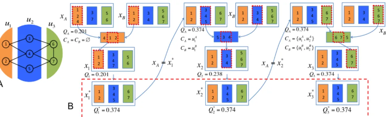
shaded nodes denote highly connected modules and the hollow nodes are for modules of which nodes have similar interaction patterns. . . . 24 3.1 An example of path generation: A. Network structure. B. Path
gen-eration procedure. . . 37 3.2 Comparison between SA and SGPG for the number of identified
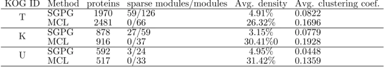
mod-ules of Hsa PPI network(A) and Sce PPI network(B) that have sig-nificantly enriched GO terms below 1%. . . 47 3.3 Percentage of different categories of modules by SGPG and MCL
(an-notated by KOG). A. KOG percentage of Sce. B. KOG percentage of
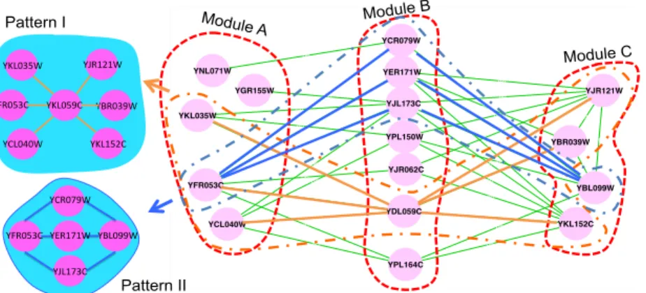
Hsa. . . 48 3.4 A subnetwork with sparsely connected modules detected by SGPG.
Module A is enriched in hexokinase activity. Module B is enriched in response to endogenous stimulus. Module C is enriched in nucleoside phosphate metabolism. . . 49 3.5 A subnetwork with sparsely connected modules detected by SGPG.
Module A is enriched in sequence-specific DNA binding with. Module B is enriched in cellular response to calcium ion. Module D is enriched in MAP kinase activity. . . 52
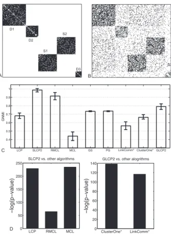
3.6 Different module identification results obtained by using P and P2. The 1st column displays three basic motifs (star motif, clique motif and bi-clique motif) (used by [86]) and the black dashed lines show the natural partitions. The 2nd column gives the P of three basic motifs and the black dashed lines denote the module dividing lines obtained by LCP. The 3rd column gives the minimum objective function values by (4.26). The 4th column gives the P2 of three basic motifs and the black dashed lines indicate the identified modules by LCP2. The 5th column shows the minimum objective function values based on (3.11). The last column illustrates the 2nd largest eigenvector ofW∗ used in Algorithm 1. . . 56 3.7 Performance comparison on synthetic networks: A. the adjacency
ma-trix of the original network; B. one example of the randomly shuffled network (obtained by shuffling half of the original edges); C. GNMI comparison among all algorithms; D. t-test results. . . 68 3.8 Statistical performance in detecting each module: A. Accscores
com-parison among all algorithms; B. t-test results based on distributions of Acc. For low bars in B, we put the −log(p−value) values on top of the bars. . . 68 3.9 The top bar figure shows the comparison results based on the F
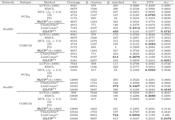
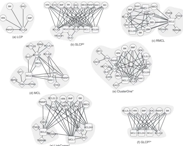
mea-sure on four PPI networks. The bottom figure displays the comparison of the percentages of matched GO terms in the complete set of selected high-level GO terms. For theHsaBioGRID PPI network, GS and PG fail to execute due to the memory limitation. . . 74 3.10 The pro-survival and cytochrome c release modules in HsaBioGRID
PPI network detected by all the algorithms (GS and PG fail to execute because of running out of memory). The pro-survial proteins are in rectangle shapes and the cytochrome c release proteins are in circle shapes. Diamond shapes denotes the proteins which belongs to neither the pro-survial proteins nor the cytochrome c release proteins. Shaded areas represent the modules detected by the algorithms. . . 75 3.11 The FGF/FGFR signaling modules in HsaHPRD PPI network
de-tected by all algorithms. FGF proteins are in the circle shapes and FGFR proteins are in the rectangle shapes. Diamond shapes indicate proteins of neither FGF proteins nor FGFR proteins. Shaded areas represent the modules detected by the algorithms. . . 77
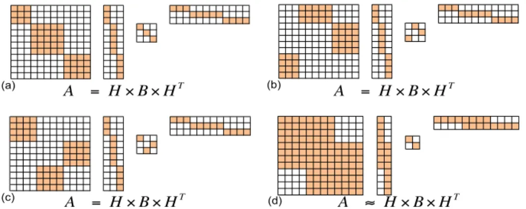
3.12 Graph clustering under different settings: (a) Toy example for com-munity detection for undirected graph. (b) Toy example for directed graph clustering. (c) Toy example for block modeling clustering. (d) Toy example for overlapping graph clustering. . . 82 3.13 Performance comparison for undirected graph clustering: (a) NMI
comparison (non-overlapping) with increasing mixing parameter µ. (b) GNMI comparison (overlapping) with increasing overlapping frac-tion valuesθ when µ= 0.1. (c) GNMI comparison (overlapping) with increasing overlapping fraction values θ when µ= 0.3. . . 98 3.14 Performance comparison for directed graph clustering: (a) NMI
com-parison (non-overlapping) with increasing mixing parameter µ. (b) GNMI comparison (overlapping) with increasing overlapping fraction values θ when µ = 0.1. (c) GNMI comparison (overlapping) with increasing overlapping fraction values θ when µ= 0.3. . . 102 3.15 (a) Underlying blockmodel structure of synthetic blockmodel
bench-marks. (b) Example of a random network with µ = 0.4. (c) NMI comparison with the increasing noise level for all the competing algo-rithms. . . 105 3.16 (a) Surface of average NMI values for every (α, β) pair. (b) Surface of
entropy scores for every (α, β) pair. . . 107 3.17 GO enrichment comparison for all the competing algorithms. . . 110 4.1 A. Network clustering separately for two networks G1 and G2; B.
Sequence similarities betweenG1 and G2; C. Joint network clustering. The width of edges in the virtual modular space is proportional to the number of aggregated edges in original networks. c2014 IEEE . . . . 113 4.2 Results for synthetic networks with a known underlying structure: A.
The structure of the virtual network. B. One example of the adja-cency matrix for a generated network at the noise level 0.5; C. One example of the similarity matrix at he noise level 0.5; D. Performance comparison. c2014 IEEE . . . 120 4.3 A. Number of modules with statistically significantly enriched GO
terms below 1% after Bonferroni correction for differentNm. B.
Num-ber of statistically significantly enriched GO terms that cover fewer than 100 proteins. c2014 IEEE . . . 122
4.4 Illustration of our proposed joint clustering algorithm. A. Construc-tion of the integrated network. B. Random walk strategy. C. Equiv-alence between a directed network (transition matrix P) and a sym-metric undirected network (transition matrix ¯P). . . 125 4.5 Performance comparison of competing algorithms for complex
predic-tion in both yeast PPI networks. A. Comparison on the number of matched reference complexes. B. Comparison on the F-measure. . . . 134 4.6 Performance comparison of competing algorithms for GO enrichment
analysis. A. GO enrichment comparison on the SceDIP network. B. GO enrichment comparison on theSceBGS network. . . 135 4.7 Comparison on the number of enriched GO terms for all the competing
algorithms in two yeast networks. . . 136 4.8 Performance comparison of competing algorithms for complex
predic-tion in both human PPI networks. A. Comparison on the number of matched reference complexes. B. Comparison on the F-measure. . . . 136 4.9 Performance comparison of competing algorithms for GO enrichment
analysis. A. GO enrichment comparison on the HsaHPRD network. B. GO enrichment comparison on theHsaPIPs network. . . 137 4.10 Comparison on the number of enriched GO terms for all the competing
algorithms in two yeast networks. . . 138 4.11 Performance comparison of competing algorithms for complex
predic-tion in the SceDIP and HsaHPRD network. A. Comparison on the number of matched reference complexes. B. Comparison on the F-measure. ASModel (Different Species) indicates the results obtained by joint clustering of the SceDIP and HsaHPRD PPI networks. AS-Model (Same Species) indicates the results obtained from joint cluster-ing of theSceDIP andSceBGS networks for yeast and joint clustering of the HsaHPRD andHsaPIPs PPI networks for human, respectively. 139 4.12 Performance comparison of competing algorithms for GO enrichment
analysis on the SceDIP and HsaHPRD networks. A. GO enrichment comparison on the SceDIP network. B. GO enrichment comparison on the HsaHPRD network. . . 141 4.13 Comparison on the number of enriched GO terms for all the competing
5.1 Degree distribution of the yeast protein interaction network extracted from DIP database. . . 144 5.2 Comparison among all competing algorithms on SGD dataset in terms
of the composite scores. CONE and LinkC are short for ClusterONE and LinkComm . . . 152 5.3 Comparison among all competing algorithms on MIPS dataset in terms
of the composite scores. CONE and LinkC are short for ClusterONE and LinkComm. . . 153 5.4 An example of a subnetwork with low conductance. The red dash line
indicates the network is separated into Gand H two parts. . . 160 5.5 A induced subnetwork G. The shade part of G is the subnetwork G0. 161 5.6 Densest subgraph examples. (a) a linear pathGl; (b) a dense graphGs.161
5.7 Duplication/divergence model for evolution of protein interaction net-works. Starting from a protein complex G1 with three proteins, after the duplication, elimination and emergence process, G1 evolves to G01 and G001. “NC” denotes the elimination or emergence of edges is un-correlated to the duplicated node u∗1. “C” denotes the elimination or emergence of edges is correlated to the duplicated node u∗1. The dash lines represent the duplicated edges. The dot lines represent the eliminated edges. And the dot dash lines represent the emerged edges. 162 5.8 Results using SGD golden standard. Shades of the same color
indi-cates quality scores of the same algorithm. The height of each bar is the value of the composite score. SceDIP, SceBioGrid, SceIntAct and SceMINT are four yeast protein interaction networks obtained from four different databases. Asterisks mark algorithms that use all four yeast protein interaction networks. CONE and LinkC are short for ClusterONE and LinkComm. . . 170 5.9 Results using MIPS golden standard. Shades of the same color
indi-cates quality scores of the same algorithm. The height of each bar is the value of the composite score. SceDIP, SceBioGrid, SceIntAct and SceMINT are four yeast protein interaction networks obtained from four different databases. Asterisks mark algorithms that use all four yeast protein interaction networks. CONE and LinkC are short for ClusterONE and LinkComm. . . 172
5.10 Comparison of composite scores for three protein complex dataset. Diamonds mark algorithms that use SceDIP and HsaDIP protein in-teraction networks. CONE and LinkC are short for ClusterONE and LinkComm. . . 175
LIST OF TABLES
TABLE Page
3.1 Parameter settings in SA and SGPG . . . 45 3.2 Comparison of SA and SGPG on Hsa and Sce . . . 46 3.3 Topological analysis of different KOG categories in Sce network . . . 48 3.4 Sparse modules in O, U and T KOG categories forSce network . . . 51 3.5 Topological analysis of different KOG categories in Hsa network . . . 52 3.6 Sparse modules in O, U and T KOG categories forSce network . . . 53 3.7 Information of the four real-world PPI networks. . . 65 3.8 Performance comparison for complex prediction onSce PPI networks. 69 3.9 Performance comparison for complex prediction onHsa PPI networks. 69 3.10 Comparison on Facebook ego network. . . 108 4.1 Information of four real-world PPI networks. . . 133 4.2 The information of the derived clusters by all competing algorithms . 133 5.1 The FLCD algorithm . . . 148 5.2 The detailed information of four yeast protein interaction networks . 149 5.3 Comparison of protein complex prediction on SGD dataset. . . 152 5.4 Comparison of protein complex prediction on MIPS dataset. . . 153 5.5 The detailed information for four yeast protein interaction networks. . 163 5.6 The detailed information for four protein interaction networks in DIP
database. . . 163 5.7 Detailed benchmark results of various algorithms on four yeast protein
5.8 Detailed benchmark results of various algorithms on four yeast protein interaction networks using the MIPS complex set. . . 173 5.9 Detailed benchmark results of various algorithms on SceDIP and HsaDIP
using the SGD complex set. . . 175 5.10 Detailed benchmark results of various algorithms on SceDIP and HsaDIP
using the MIPS complex set. . . 175 5.11 Detailed benchmark results of various algorithms on SceDIP and HsaDIP
using the CORUM complex set. . . 176 5.12 GO consistency and coverage comparison of all competing algorithms
on DIP dataset. . . 178 5.13 GO consistency comparison between ClusterM and OrthoClust. . . . 179 5.14 Comparison of protein function prediction for all competing algorithms.180
1. INTRODUCTION∗
What is the next big wave in technology? Different people may have different opinions. Let us look at the Internet giant — Google’s next move. Along with the lines of self-driving cars and smart glasses, Google’s newest venture is called California Life Company, whose goal is to extend human’s life by 20 to 100 years. It seems unreal, however, the request to live a little bit longer has been in demand from the beginning of the human society. Actually, the investigations of one kind of flatworm have shed light on the possibilities of alleviating aging in human cells since researchers have demonstrated that the flatworm can overcome the aging process and could potentially live forever [103]. However, to enforce the mission impossible, several fundamental questions need to be answered in advance, such as what is the molecular mechanism of an organism and how the molecular mechanism controls the activities within the organism.
To unveil the mystery of those basic biological problems through understanding their underlying cellular mechanism, it is indispensable to look into the Deoxyri-bonucleic acid (DNA), which is a molecule that stores the genetic instructions used in all biological processes of all known living organisms. Human Genome Project (HGP) has achieved tremendous success in determining the DNA sequence and rec-ognizing and mapping genes of the human genome based on both their physical and functional responsibilities. However, HGP collaborated all research pioneers around the world and still costed 13 years and $3 billions, which illustrates how difficult to sequence a general genome in the last decades. With the help of fast development ∗Fig 1.1 in this chapter is reprinted with permission from “Wisdom of crowds for robust gene network inference” by Daniel Marbach, James C Costello, Robert Kffner, Nicole M Vega, Robert J Prill et al, Nature Method, 9(8): 796-804, 2012, Copyright 2012 by Nature Method.
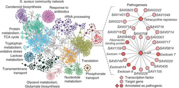
Figure 1.1: An example for module identification for a gene co-expression network.
of high-throughput technologies, nowadays, obtaining biological data, such as ge-nomics data, proteomics data and molecular interactions becomes more efficient and less expensive. Some widely used high-throughput technologies are next-generation sequencing, mass spectrometry, yeast two-hybrid assays and microarrays. Due to the availability and diversity of the high-throughput technologies, there are tons of biological data generated every day, which brings biologists into a brand-new era with the biological data they have never had in the past.
The dramatically increasing generation of biological data enables us to better un-derstand biological systems. Identifying functional modules in biological systems is a fundamental way to comprehend the functional organizations of the corresponding biological systems and interpret their underlying mechanisms. Biologically, a func-tional module in a biological system consists of a group of biological units, which perform similar functions. In this dissertation, we focus on identifying functional modules in biological systems, which are modeled as biological networks constructed
from interactome data. Fig. 1.1 shows an example of module identification in a gene co-expression network [59]. The modules in the networks are identified barely based on the topological structures. The functional organization and topological relationships between modules are clearly illustrated through module identification.
1.1 Biological networks
Complex biological systems can be represented and investigated as networks. In general, a node of a biological network represents a protein or a gene and an edge indicates the association between nodes. Based on different purposes and different biological systems, different types of networks are generated. For example, there are protein-protein interaction networks, transcript-transcript association networks (gene co-expression networks) and DNA-protein interaction networks (Gene regula-tory networks).
For all kinds of theses biological networks, a principle, called guilt-by-association, is widely used. Guilt-by-association declares that the nodes (biological units) in the biological networks, which are connected by an edge, are more likely to perform the same function than nodes (biological units) not linked together. Therefore, it is possible to predict the function of an unknown node (biological unit) through the functions of its topological neighborhood, which have been validated either by chemical experiments or biological experts.
Because complicated biological systems are abstracted into biological networks, basic biological problems are converted to network related problems. Therefore, the challenges over the next decades are to make use of the information existing in the biological networks to answer fundamental biological problems [78], such as func-tional organization and robustness of biological systems. Here we briefly introduce two kinds of widely used biological networks, which are protein interaction networks
and gene co-expression networks.
1.1.1 Protein interaction networks
Proteins are large molecules composed of one or more connected amino acid residues. They carry out diverse functions within living organisms. Biologically, proteins rarely act alone. Through protein-protein interactions, groups of proteins are organized together to facilitate diverse fundamental molecular processes within a cell.
Protein-protein interactions in a cell construct a protein interaction network, where nodes represent proteins and edges represent physical protein-protein inter-actions. Thanks to the high-throughput technologies, all physical protein-protein interactions in a cell can be screened in one test. There are many ways to detect the physical binding interactions. The most widely used high-throughput methods of detecting the physical protein-protein interactions are yeast two-hybrid screening (Y2H) [38] and affinity purification coupled to mass spectrometry (AP-MS) [114]. Y2H was proposed by Fields and Song in 1989 [88]. Pairwise protein interactions with binary weights can be inferred by Y2H. In Y2H, the transcription factor is separated into two fragments, which are called binding domain and activating do-main. The binding domain is fused onto a protein of interesting (referred as the bait protein) and the activating domain is fused onto another protein (referred as the prey protein). If the bait protein and prey protein interacts with each other, then the activating domain is brought to the transcription start site, which incurs the occurrence of the transcription of reporter genes. If those two proteins do not interact, then there is no occurrence of the transcription of reporter genes. Based on the occurrence of the transcription of reporter genes, the interactions between proteins can be identified. The limitation of Y2H is that the number of identified
protein-protein interactions is low due to the loss of transient protein interactions in purification steps. AP-MS consists two steps. In the AP (affinity purification) step, a protein of interest, called bait, is affinity caught in a matrix. The bait protein is passed through the matrix, the protein, interacting with the bait protein, is retained due to interaction with the bait. After purification, proteins can be analyzed by MS (mass spectrometry), which is a chemistry technique that helps to determine the amount and type of chemicals in a sample [114]. There are other profiling techniques to detect protein-protein interactions, however, the interactions identified by those methods are noisy [73].
There are many public protein interaction databases available for researchers and scientists. Some databases such as BioGrid [101], DIP [90] and IntAct [41] contain protein interaction networks of many different species. Some databases only maintain protein interaction networks of specific species, such as HPRD [82] (a database for human protein interaction network) and FlyBase [27] (a database for fruit fly protein interaction network).
1.1.2 Gene co-expression networks
Similar to protein interaction networks, gene co-expression networks are also net-work with symmetric interactions, where each node represents a gene and each edge indicates the similarity of the co-expression patterns of a pair of genes with respect to samples. Gene co-expression networks are of biological interest because co-expressed genes may be controlled by the same transcriptional regulatory mechanism, or the same pathway or protein complex.
The construction of a gene co-expression networks follows a two-step approach. In the first step, the similarity between every pair of gene expression data is calculated. Then in the second step, edges with small similarities are filtered out by setting a
threshold value. The input data for formulating a gene co-expression network is stored in a matrix format. For example, in a microarray experiment, we can obtain the gene expression values of mgenes andn samples, then the input data is am×n
matrix, which is called the expression matrix. Each row in the expression matrix implies the gene expression pattern of that gene. In the first step, we can estimate the similarity of the gene expression patterns between pairwise genes through computing the similarity between two row vectors. Pearson’s correlation coefficient, mutual information, spearman’s rank correlation coefficient and Euclidean distance are the four mostly used co-expression measures [102]. After the calculation of the similarity scores, we obtain an m ×m similarity matrix, each element of which shows how similar two genes change together with respect to expression levels. In the second step, the elements of them×msimilarity matrix are dichotomized based on a certain threshold. The dichotomized matrix is the adjacency matrix of the gene co-expression network. “1” in the adjacency matrix denotes two genes are correlated under the same samples or conditions, and “0” otherwise.
1.2 Challenges
Although there are many algorithms developed to identify functional modules in different types of biological networks, efficient algorithms still need to be devised to detect modules with better accuracy and less computational time. Here we summa-rize the challenges we encountered.
1.2.1 What is the good definition of a functional module?
Intuitively, based on interactome data, if two nodes interact with each other, they are more likely to share the same cellular functionalities than nodes that do not interact. Thus, densely connected subnetworks in a given network can be viewed as potential functional modules. Based on this idea, many algorithms have been
suc-cessfully applied to identify functional modules in biological networks by detecting “higher than expected connectivity” subnetworks based on modularity optimiza-tion [75, 74] or random walk on graphs [105, 91, 93, 68].
However, in addition to densely connected modules in biological networks, such as protein complexes, there are other topological structures that may possess im-portant cellular functionalities. Again, based on interactome data, the nodes that interact with similar sets of other nodes in a given network also intuitively have a higher probability of sharing the similar functionalities compared to the nodes that do not share any interacting partners or neighbors [80, 86, 64]. These nodes may not directly interact with each other but they still work towards similar cellular functionalities and hence should belong to the same modules. It is well known that transmembrane proteins, such as receptors in signal transduction cascades, tend to interact with cytoplasmic proteins as well as with extra-cellular ligands, but rarely interact with themselves [80]. To identify such types of functional modules, many state-of-the-art block modeling module identification algorithms have been proposed recently [67, 66, 86, 35]. But those algorithms suffer from the prohibitive computa-tional complexity due to the inherent combinatorial complexity of the block modeling problem. Therefore, more efforts need to be made to develop algorithms that can efficiently identify functional modules based on nodes interaction patterns.
1.2.2 Degree heterogeneity
The degrees of nodes in a biological network obey the power-law distribution: therefore, there exist many nodes with low degrees and few nodes with high degrees, which is called degree heterogeneity. Due to degree heterogeneity, it is hard to design module identification algorithms with the presence of the nodes of very low degrees. Several algorithms are developed for power-law networks but most of them have not
been applied on biological networks [20], and most algorithms designed for biological networks do not consider the degree heterogeneity problem [80, 86, 64, 75, 74, 91, 93].
1.2.3 Biological experiment noise
Currently, the biological interactions in the biological networks generated by high-throughput experiments are very noisy. For example, it is well known that there are lots of false positive and false negative interactions presented in the protein inter-action networks [21]. Therefore, module identification simply based on individual biological networks may not be able to yield robust and accurate results. We may need to appropriately integrate other available information in addition to network topology, such as sequence and function similarity, to repress the noise. Comparative analysis of multiple biological networks enable us to borrow topological information across networks and incorporate the corresponding homological information to re-duce the influence of noise. Many algorithms [22, 94, 46, 39, 116] have been developed to find conserved modules in multiple networks.
1.3 Our contributions
We develop efficient computational algorithms to overcome the challenges dis-cussed in the previous section.
1.3.1 Module identification based on interaction pattern
To discover modules with richer topological structures, we devise a novel sub-gradient method with heuristic path generation [109] to accelerate the optimization process for the block modeling formulation [80]. To overcome the resolution prob-lem [30] of the block modeling formulation [80], we propose an algorithm SLCP2 [110] based on two-hop random walk strategy to identify fine-size functional modules con-sidering the interaction patterns. Additionally, we propose an non-negative matrix
factorization (NMF) based framework for more general module identification prob-lems by sparse regularized. We discuss these algorithms in more details in Chapter 3.
1.3.2 Overcoming the degree heterogeneity
We devise a new local algorithm that can identify densely connected modules with the existence of low-degree nodes. This new algorithm consists two local steps guided by optimization principles. The algorithm first searches for a low-conductance set near a node, which is well separated from the rest of the network and then identifies the densest sub-network in the low-conductance set to get rid of the low-degree nodes. This new algorithm with such a principle-guided seed expansion and shrinking procedure outperforms state-of-the-art module identification algorithms in biological networks. We present this new algorithm and experimental results in Chapter 5.
1.3.3 Identifying conserved modules in multiple networks
We incorporate homological information across networks to repress the noise in each individual networks. We extend the block modeling formulation and two-hop random walk strategy to search functional modules based on interaction patterns in pairwise biological networks [112], which are discussed in details in Chapter 4. Furthermore, in Chapter 5, we develop an novel algorithm to identify conserved modules in multiple networks, which are topological cohesive and possess many-to-many homological correspondences.
Before we getting into the details of our developed module identification algo-rithms, we first introduce the background, basic mathematics notations, and related work to the module identification problem.
2. RELATED WORK∗
In this chapter, we review the state-of-the-art module identification algorithms for both individual networks and multiple networks. For individual networks, we first go through methods of identifying topological cohesive modules and then re-view algorithms that search functional modules based on interaction patterns. For multiple networks, we survey the state-of-the-art methods for pairwise and multiple networks, respectively, based on how they representing multiple networks [89, 54, 99, 46, 22, 94, 39, 116].
2.1 Module identification for topological cohesive modules
To identify topological cohesive modules, many algorithms have been successfully applied based on modularity optimization [75, 74]. Additionally, several algorithms based on Markov random walk on networks also have been proposed recently. For example, Markov CLustering (MCL) algorithm is one of such module identification algorithms for biological network analysis by iteratively implementing “Expand” and “Inflation” operations on the transition matrix of the underlying Markov chain of random walk [26]. Regularized MCL (RMCL) [91, 93] further extends the original MCL algorithm to penalize the large cluster size at each iteration to obtain more balanced modules with a similar number of nodes within them. Other formulations based on Markov random walk, including finding low conductance sets [105], also can be applied in module identification, which is in fact similar to normalized cut prob-lems [115] in graph partitioning to minimize the normalized cut size across modules. Recently, several overlapping module identification methods have been developed to ∗Fig 2.3 in this chapter is reprinted with permission from “A novel subgradient-based optimiza-tion algorithm for blockmodel funcoptimiza-tional module identificaoptimiza-tion” by Yijie Wang and Xiaoning Qian, BMC Bioinformatics, 14(Suppl 2): S23, 2013, Copyright 2013 by BMC Bioinformatics.
detect densely connected modules that may overlap with each other in networks. For example, ClusterOne (CONE) [68] can be viewed as the overlapping version of nor-malized cut. LinkComm (Link community) [1] formulates the overlapping module identification in an innovative framework to implement the hierarchical clustering on edge graph representations, which reveals hierarchical and overlapping organization of networks.
In this section, we review the representative definitions of a topological cohesive module, such as modularity and conductance, and the corresponding algorithms. Assuming we have a biological network in graph representation G(V, E), where V is the set of |V| =n nodes representing proteins or genes, and E ={eij} is the set of
|E|=m edges, which suggest the physical interactions or correlations. The network
Gcan be presented by an adjacency matrixA, whose elementAij of which equals 1 if
there is an edge between nodesiandj and 0 otherwise. We only consider unweighted networks with binary edge weights. D is a diagonal matrix withDii= deg(i), where
deg(i) = P
jAij is the degree of nodei. The goal of module identification is to detect
a group of nodes, which perform similar functions or possess identical properties, barely based on the network topologies.
2.1.1 Community detection based on modularity
Community detection is one of the major directions of functional modules iden-tification. Community detection aims to identify groups of nodes that are densely connected inside and loosely connected outside. Intuitively, a good community in networkG(V, E) should be a group of nodesC such that there are many more edges between the nodes in C than from the nodes in C to nodes in V −C. One impor-tant definition that has been intensively studied for community detection is called modularity [74].
2.1.1.1 The definition of modularity
Basically, modularity expresses the relationship between the actual connectivity inside a group of nodes C and the expected connectivity in C. The formal mathe-matical formulation of the modularity of C is
QC =
X
ij
[Aij −Pij]δ(gi, gj), (2.1)
where gi denotes the community that nodei belongs to and δ(s, t) = 1 if s =t and
0 otherwise. Pij is the expected number of edges between nodesi and j. Matrix P
can be considered as the weighted adjacency matrix of a null model, which has the same number of nodes in G. P should satisfy the following constraints. First, P is symmetric, which implies Pij =Pji. Second, QC = 0 when all nodes are placed in a
single group. Setting all gi ∈C, we have
X ij [Aij −Pij] = 0⇒ X ij Aij = X ij Pij = 2m. (2.2)
Physically, the equation means that the expected number of edges in the entire null model equals the number of actual edges in G. Additionally, we require the degree distribution of the null model is approximately the same to the original network G. Hence, we need
X
j
Pij =di, (2.3)
where di is the degree of node i. One widely used null model, which satisfies the
conditions above is
Pij =
didj
2m. (2.4)
commu-nities {G1, G2, ..., Gk} in G by maximizing the corresponding modularity. For this
k-way partition, node ican be assigned to gi ={1,2, ..., k}. Then the maximization
of modularity can be written as
max :X
ij
X
gi,gj
[Aij −Pij]δ(gi, gj). (2.5)
Obviously, (2.5) is a combinatorial optimization problem, which is computational intractable by exhaustively searching all possible k partitions in G. However, many algorithms [74, 13, 2] have been proven effective. Prof. Mark Newman, who origi-nally proposed the definition of modularity, developed a method to approximate the solution of (2.5) [74] by using the eigen-system of matrix A−P. Blondel devised a greedy method to handle large-scale networks with good solution quality [13]. [2] extended the column generation methods for mixture integer programming to find the exact solution of (2.5).
2.1.1.2 The algorithm based on eigenvectors
Here, we briefly review the community detection method using eigenvectors by Newman [74]. Following [74], we define a binaryn×k community assignment matrix
X, where theith row indicates the membership of nodeiand thejth column presents the jth community. Formally,
Xij =
1 if node i belongs to communityj,
0 otherwise.
(2.6)
Noticing that the δ function in (2.5) is equivalent to δ(gi, gj) = k X l=1 XilXjl. (2.7)
Then (2.5) can be written as
Q=X ij X gi,gj [Aij −Pij]δ(gi, gj) = n X i,j=1 k X l=1 [Aij −Pij]XilXjl =Tr(XTBX), (2.8)
where B =A−P. There is an implicit constraint for the above problem, which is
X is a binary assignment matrix with P
jXij = 1 and
P
lXliXlj = 0,∀i6=j.
Because B is a symmetric matrix, hence, it can be diagonalized B = UΛUT, where U = (u1|u2|...) is the matrix of eigenvectors of B and Λ is a diagonal matrix of eigenvalues Λii=βi. B may not be positive semi-definite matrix, which means βi
may be negative. To alleviate the influence of the negative eigenvalues, we do the following transformation
Q= Tr(XTBX) = Tr(XTUΛUTX)
=αn+ Tr(XTU(Λ−αI)UTX).
(2.9)
Here we make use of the fact that Tr(XTX) = n and α is related to the negative
smaller than α, then the above equation becomes Q=αn+ Tr(XTU(Λ−αI)UTX) ≈αn+ Tr(XTUp(Λp −αIp)UpTX) =αn+ k X l=1 p X j=1 n X i p βj −αUijXil !2 (2.10)
We definen p-dimensional vectorsri =
p
βj−αUij to characterize each nodeiin G.
ThenPp j=1 Pn i p βj −αUijXil 2 =Pp j=1 P i∈Gl[ri]j 2
=|Rl|2, whereRlis the sum
of all p-dimensional vectors that belongs to community l. Finally, the modularity Q
can be approximated by Q≈αn+ k X l=1 |Rl|2. (2.11)
Therefore the maximization of modularity is converted to clustering the nodes in
G into groups so as to maximize the magnitudes of the vectors Rl, which is called
vector partition problems. The k-means algorithm can be easily applied to solve the vector partition problem.
2.1.1.3 The resolution problem
Identification of communities for biological and social networks using modularity has been proved effective by many researchers [16, 55]. However, [30] pointed out that using modularity can not resolve some small-size meaningful modules. There-fore, identification of modules like protein complexes in protein interaction networks becomes the bottle-neck for modularity based algorithms.
2.1.2 Community detection based on conductance
Another definition that can help us identify community structures in G is con-ductance [6]. Concon-ductance measures how fast a random walk on G converges to the
stationary distribution. For a set of nodes C, its conductance is defined as
φ(C) = |E(C, ¯
C)|
min{vol(C),vol( ¯C)}, (2.12)
where vol(C) = P
i∈Cdeg(i) and |E(C,C¯)| denotes the connections between sets C
and ¯C = V −C. Finding S with the minimal conductance is called conductance minimization. In this section, we will discuss several algorithms [95, 6, 26], which are closely related to conductance.
2.1.2.1 Normalized cut
For a setC, the normalized cut [95] is defined as
Ncut(C) =
|E(C,C¯)|
vol(C) . (2.13)
Comparing (2.13) with (2.12), obviously, only the denominator is different. When dividingGinto large enoughkparts{V1, V2, ..., Vk}, reasonably assuming at each
par-tition vol(Vi) <vol( ¯Vi), these two definitions are equivalent. Therefore, normalized
cut can be viewed as a special case of conductance.
X is the module assignment matrix and hi presents the ith column of X. X is
in the following feasible solution space
Fk ={X :X1k =1n, Xij ∈ {0,1}}. (2.14)
Detectingk normalized cuts can be formulated as X i Ncut(Vi) = X i |E(Vi,V¯i)| vol(Vi) =X i xT i (D−A)xi xT i Dxi = Tr xT1(D−A)x1 xT 1Dx1 0 0 0 x T 2(D−A)x2 xT 2Dx2 0 0 0 ... k×k = Tr(XTDX)−1XT(D−A)X (2.15)
Our goal is to find the optimal solution X that can minimize the k-way normalized cuts. The problem can be casted into the following optimization problem:
min : Tr(XTDX)−1XT(D−A)X s.t. X ∈ Fk.
(2.16)
Furthermore, we find that the above problem can be further simplified to the follow-ing equivalent problem
max : Tr
(XTDX)−1XT(A)X
s.t. X ∈ Fk.
(2.17)
we finally have max Tr(YTW Y) s.t. YTY =Ik, (D−1/2yj)i ∈ {0, s−1j },∀i, j, Y S1k= diag(D−1/2), S = Diag(s1, s2, ..., sk)∈Rn+. (2.18)
The above problem is a NP-hard combinatorial optimization problem.
Spectral method
A spectral method can be used to approximate the solution of (2.20). Consider the following relaxed problem of (2.20)
max Tr(YTW Y)
s.t. YTY =Ik.
(2.19)
Although Tr(YTW Y) is not convex because W may not be positive semi-definite
matrix, we can retrieve the optimal solution supported by Kay Fan theorem. Based on the theorem, the optimal Y∗ is attained at Y∗ = Uk, whose columns are the
eigenvectors corresponding to thek largest eigenvalues ofW. k-means clustering can be used to obtain a feasible solution in the original constraint set.
Ky Fan Theorem: Let T be a symmetric matrix with eigenvalues λ1 ≥λ2 ≥...≥λn
and the corresponding eigenvectors U = (u1, ..., un). Then k X i=1 λi = max XTX=I k Tr(XTT X) (2.20)
Moreover, the optimal X∗ is given by X∗ = [u1, ..., uk]Q with Q being an arbitrary
Other methods
Thek normalized cut problem (2.13) can also be solved by semi-definite program-ming [95]. For finding the exact solution, one can reformulate (2.13) into a mixture integer programming and solve it by using linear programming toolbox [28].
2.1.2.2 Local algorithm based on personalized PageRank vector
Andersen [6] developed a local algorithm, called PageRank-Nibble, to find a low-conductance set near a specific starting node in the network based on a personalized PageRank vector. The conductance of the setCidentified by the algorithm is at most
f(φ(C)), where f(φ(C)) is Ω(φ(C) 2
logm ) (m: the number of edges in G). Furthermore,
the local algorithm can find C in time O(mlog 4
m
φ(C)3 ). PageRank-Nibble provides us a powerful weapon to find a low-conductance set near a specific node with theoretical guarantee with only linear computational complexity with respect to |C|.
Algorithm: ApproximatePageRank (i, α, ξ) Letp=0 and r=ei.
While maxi∈V
r(i) deg(i) ≥ξ
Choose a node i with r(i) deg(i) ≥ξ. Apply push(i, p, r) and update pr, r. Return p≈pr(α, ei).
Figure 2.1: The algorithm to approximate the personalized PageRank vector.
Approximation of a personalized PageRank vector
One fundamental step of PageRank-Nibble is to approximate the personalized PageRank vector around nodei. Following [6], the lazy variation of PageRank vector
is defined as
pr(α, s) =αs+ (1−α)pr(α, s)P, (2.21) where α is a constant in (0,1] called the teleportation constant, s is a distribution called preference vector and P = 1
2(I −D
−1A) is the transition probability matrix of the lazy random walk on G. The personalized PageRank vector used in (2.21) requiress=ei, whereei is an all zeros vector with one on theith entry, meaning that
the preference vector concentrates on theith node. The pseudo code of the approxi-mation is displayed in Fig. 2.1, where the subroutine used is shown in Fig. 2.2. The technical and theoretical details can be found in [6]. The approximation algorithm has the proven guarantee: maxi∈V
r(i) deg(i) ≥ξ. Algorithm: push(p, r) Letp0 =p and r0 =r. p0(i) = p(i) +αr(i). r0(i) = (1−α)r(i) 2 . For nodej (Aij = 1), r0(j) = r(j) + (1−α) r(i) 2deg(i). Return p0 and r0.
Figure 2.2: The push algorithm.
PageRank-Nibble
Once we obtain the approximation of personalized PageRank vectorpnear node
i, then we can sort the nodes around i base on p(j)
deg(j). Assuming v1, v2, ..., vN p is the ordering of the nodes around i such that p(vi)
deg(vi)
≥ p(vi+1)
deg(vi+1)
, we compute the conductance of the set Cj = {v1, v2, ..., vj}, j ∈ {0,1, ..., Np}. The set C∗ with the
smallest conductance C∗ = arg min
Cj
φ(Cj) is the result produced by the PageRank
2.1.2.3 Markov clustering algorithm (MCL)
MCL [26] is a graph clustering algorithm based on manipulation of transition probabilities between nodes of the graph. The underlying principle of MCL is still unknown, which has not prevented its successes on many real-world applications. We category MCL as a algorithm related to finding low-conductance sets in network because its similarity to Nibble [100]. Nibble is a local clustering algorithm to recover the low-conductance set C around node i, whose running time is almost-linear with respect to |C|. Actually, the PageRank-Nibble algorithm is a variation of Nibble.
MCL iteratively implements “Expand” and “Inflation” operations on the transi-tion matrix P of the underlying Markov chain of random walk on the given network
G. In the “Expand” step, we perform Pt= Pt−1Pt−1. “Inflation” operation follows to computePt(i, j) = Pr t(i, j) Pn i=1P r t(i, j)
. Those two operations iterate untilPtconverges.
Each row of Pt contains the membership information corresponding to one cluster.
Generally, most of the rows of Pt converge to all zero vectors. The only parameter
of MCL is r, which controls the size of the modules in average sense. If r is large, then the module size tends to become small.
In comparison to MCL, Nibble also consists of two major steps, which is the random walk propagation and the removal of unrelated nodes. Nibble computes the random walk probability vector within the first several steps. It starts with vector q0 = ev. In the random walk propagation step, qt = Pqt−1 is performed. In the removal step, the nodes with probabilities smaller than ε ·deg(i), where ε =
φ2/(log3m2b), are zero out.
Comparing MCL with Nibble, intuitively, both of them have two similar steps, random walk propagation and node deletion. The similarity may explain why MCL yields reasonable results.
2.1.3 Community detection based on non-negative matrix factorization
Recently, NMF has been successfully applied to network partition problem [47, 24, 106, 19]. The authors in [24, 47] proposed to decompose the adjacency matrix of a network with undirected edges into symmetric non-negative components to iden-tify communities under the assumption that all modules consist of highly connected nodes. Further investigation has demonstrated its potential for detecting overlapping modules in networks [24, 76, 120].
The authors in [47, 24] propose to decompose the corresponding adjacency matrix
A for a given network into symmetric components for community detection:
min: X≥0 Γ(X) = A−XXT 2 F, (2.22)
where X is a non-negative matrix of size n×k and k is the number of potential modules. X can be naturally interpreted as the module assignment matrix. A multiplicative updating algorithm SymNMF MU [24] has been proposed to solve this problem (2.22). Xik ←Xik 1−γ+γ (AX)ik (XXTX) ik , γ∈(0,1] (2.23)
However, SymNMF MU may not converge to a stationary point. SymNMF NT [47] is a Newton-like algorithm, which solves the problem (3.17) by lining up the columns ofX. SymNMF NT converges to a stationary point. However, it has relatively larger memory consumption requirement [47].
2.2 Module identification based on interaction patterns
There are many algorithms developed to identify functional modules with the consideration of interaction patterns. For example, Power Graph (PG) [86] greed-ily collects topological similar nodes into the same module based on Jaccard Index similarity. Graph Summarization (GS) [67, 66] uses the minimum description length principle to group nodes with similar interaction patterns. However, both PG and GS are solved by greedy algorithms, which can not guarantee the global optimality. Additionally, they tend to over-segment the network to get relatively small modules based on our empirical experience. A Bayesian framework [35] based on a stochas-tic block modeling formulation has been developed to identify modules as well as the optimal number of modules. However, the algorithm only guarantees to con-verge to local optima. Reichardt [84] has proposed to solve block modeling module identification by optimally mapping the given network to an image graph using sim-ulated annealing (SA), and several optimization strategies also have been proposed to accelerate the original SA algorithm [107, 108]. NMF based optimization frame-works [106, 19] are proposed to find functional modules by explicitly considering the underlying image graph of a network, however, there is no convergence guarantee for the developed algorithms. In this section, we review the optimization formulations of block modeling.
2.2.1 Block modeling based on the image graph
We first review block modeling module identification by functional role decom-position proposed by [85, 83, 80]. For module identification of network G, we search for a non-overlaping module mapping τ which assigns n nodes in V to q different modules: τ : V 7→ U, in which U = {u1, . . . , uq} represent the module space—a
G M Ancestor network (image graph) u1" u2" u3" u4" u5"
Figure 2.3: Mapping to the module space as an introduced image graph. The shaded nodes de-note highly connected modules and the hollow nodes are for modules of which nodes have similar interaction patterns.
[85, 83, 80] introduce the virtual image graph M = {U, I} in the module space to preserves the original network interactions by the edges I. Note that when q = n, the obvious optimal image graph is the network itself.
Mathematically, the optimalτ should minimize the mismatch between the given network G and the introduced image graph M. Suppose we have the adjacency matrix of the image graph by B, whereBrs records the interaction between module
nodes ur and us. In order to make the image graph Bτiτj match the network Aij
as much as possible, we search for the optimal module mapping τ and minimize the following error function [83, 80]:
E(τ, B) = 1 M N X i6=j (Aij−Bτiτj)(wij−pij),
in which wij denotes the weight given to the edge between node vi and vj (in this
paper wij = 1 when node vi and vj have an interaction, and wij = 0 otherwise);
M = PN
i6=jwij is used to bound the error function between 0 and 1; (wij −pij)
denotes the error made on the edge between vi and vj with pij as the penalty for
the mismatches of the corresponding absent edges. Self-links in the original network are not considered with both wii = 0 and pii = 0. Typically, pij is chosen to make
the total mismatches error on existing edges (wii > 0) equal that on absent edges
(wii= 0):
PN
i6=jAij(wij−pij) =
PN
i6=j(1−Aij)pij. In order to guarantee this equality,
we follow one of possible choices [83] to let pij =
P
k6=iwikPl6=jwlj
P
k6=lwkl .
From the equation of E(τ, B), we find that Bτiτj =Aij, which means the image
graph preserves an edge (either existing edge or absent edge) in the original network, leads to E(τ, B) = 0. Otherwise, Bτiτj 6= Aij, which means image graph does not
preserve an edge in original network, leads toE(τ, B) = pij when miss-matching the
absent edge orE(τ, B) =wij−pij when miss-matching the existing edge. By further
investigating E(τ, B), we find that minimizing E(τ, B) is equivalent to maximize 1
M
PN
i6=j(wij−pij)Bτiτj which can be rewritten as maxτ,B
1 2M
PN
i6=j(wij−pij)(2Bτiτj−1)
by using binary trick. Furthermore, we can formulate the objective function as
Q(τ, B) = 2M1 P
r,s
PN
i6=j(wij −pij)δτirδτjs(2Brs−1). For the original nodes assigned
to module node ur and us by τ, we have the corresponding term as PNi6=j(wij −
pij)δτirδτjs(2Brs−1), in whichδτir is the indicator function that takes 1 when τi =r
and 0 otherwise. It is clear that the optimal solution for Brs with a given τ is to
setBrs= 1 when its corresponding term
PN
i6=j(wij−pij)δτirδτjs is larger than 0, and
0 otherwise. Hence, the optimal solutions of τ and B are naturally decomposed. The optimal image graph B can be derived in a straightforward way once we have the optimal module mapping τ, which maximizes the following equivalent objective
function: Q∗(τ) = 1 2M q X r,s N X i6=j (wij−pij)δτirδτjs . (2.24)
The maximization problem (2.24) is NP hard as it can be polynomially trans-formed to the classical quadratic assignment problem [61]. In [80], SA has been applied for the optimization, in which the time complexity increases quadratically with increasing q. While in practice, the search space for annealing parameters gets larger with increasingq too, and it can obtain high quality results only for very slow cooling schedules. For a large q (≥100), SA will be a time-consuming procedure.
2.2.2 Block modeling based on NMF
For block modeling module identification, one recent algorithm—BNMF [19]— has been derived base on the following formulation:
min: X≥0,0≤M≤1 A−XM XT 2 F +λ Mideal−M 2 F, (2.25)
whereM andMideal represent the adjacency matrices of the introduced image graph and the “ideal image matrix”, respectively. Mideal is the function of M, which is defined by Mijideal = argmin
u∈{0,1}
|u−Mij| and approximated by a sigmoid function in
the proposed projected descent algorithm. However, there is no convergence proof provided for BNMF.
2.3 Module identification for multiple networks
It is well known that protein interaction networks are noisy. There exist many false positive and false negative edges. Therefore, it is very challenging to assign func-tional roles to proteins and separate true protein-protein interactions from false posi-tive interactions. Across species comparison may provide us a valuable framework to
address those challenges. Finding conserved modules in biological networks of multi-ple species has attracted researchers attention due to its capacity of identifying net-work regions that conserved in their sequences and interaction patterns across species. Algorithms of pairwise and multiple networks [89, 54, 99, 46, 22, 94, 39, 116] have been successfully applied for searching conserved pathways and complexes. Align-Nemo [22], NetworkBlast [94] and MaWISh [46] can only handle pairwise networks by constructing pairwise networks into alignment networks. NetworkBlast-M [39] and OrthoClust [116] can deal with multiple networks but suffer from the low coverage and the resolution problems [30], respectively.
The most challenging part of finding conserved modules across networks, again an NP hard problem, is how to compromise between the time and space complexities of the algorithms and the accuracy of the alignment results. One fundamental problem is the data representation of multiple networks. Based on different data represen-tations, different algorithms are designed to solve the difficult tasks. Therefore, we go through the state-of-the-art algorithms by the ways they integrate the multiple networks.
In this section, a set ofK networksG ={G1(V1, E1), G2(V2, E2), ..., GK(VK, EK)}
is presented by a set of adjacency matrices A={A1, A2, ..., AK}, and the orthology
relationships between them are kept in S, where S(i, j),∀i ∈ Gs, j ∈ Gt is the
orthology correspondence between node i in network Gs and node j in network Gt.
For algorithms using pairwise networks, a pair of networks {G1, G2} and their orthology relationship S12 are represented by a product graph, which is the Carte-sian product of the two networks containing every possible combinations between nodes across species. [54, 99] are developed based on the product graphs. An alignment network consists of nodes across networks with orthology correspondence and edges, which are the conserved interactions. The alignment network is the
ba-sic data representation for many state-of-the-art pairwise networks alignment algo-rithms [99, 46, 22, 94]. Researchers extend pairwise networks alignment to multiple networks alignment by representing the integration of G and S using a K layer graph [39, 116], which is also called layered alignment graph GH(∪iVi, E) where E
is the union of ∪iEi and EH denoting inter-layer edges corresponding to S. The
existing multiple networks alignment algorithms [39, 116] are based on K layered alignment graphs due to computational considerations.
2.3.1 Algorithms based on the product graph
LetGa andGb be two biological networks to align. Two networks hasNa and Nb
nodes respectively. We define B ∈R(Na×Nb)×(Na×Nb) as the Cartesian product graph GB fromGa and Gb: B =Ga⊗Gb. Denote the all one vector 1∈RNa×Nb and
¯
B =B×Diag(B1)−1, (2.26)
where Diag(B1) can be considered as a degree matrix with B1 on its diagonal and all the other entries equal zero. B¯ is the transition probabilities for the underly-ing Markov random walk in IsoRank [99]. It is well known that if Ga and Gb are
connected networks and neither of them is bipartite graph, then the corresponding Markov chain represented by ¯B is irreducible and ergodic, and there exists a unique stationary distribution for the underlying state transition probability matrix ¯B.
2.3.1.1 IsoRank
[99] IsoRank is a pairwise network alignment algorithm based on random walk on the product network GB. IsoRank is derived based on the intuition that a pair
of nodes is aligned together if their neighborhood nodes aligned together. Instead of finding the alignment directly, IsoRank first computes the similarities between all
node pairs in two networks based on their neighborhood topologies and sequence in-formation. The all-to-all similarity scores can be obtained by finding a right maximal eigenvector of the matrix ¯B: ¯Bx=xand 1Tx= 1, x≥0. When two networks are
of reasonable size, spectral methods as well as power methods can be implemented to solve the eigen-system. When we obtain r, a bipartite network on networks Ga
andGb can be constructed, edges of which are the similarities scores stored inr. The
alignment result of IsoRank then can be attained by solving the maximal matching problem in the bipartite network.
2.3.1.2 IsoRankN
[54] IsoRankN is the extension of IsoRank. Computationally, it is very hard to store the product network of three or more networks. For example, for three 100-node networks, the size of the product network of them is 1000,000× 1000,000. The size of real-world networks are much larger than 100, therefore it is memory prohibitive to use the product network for multiple networks alignment problem. Instead, Iso-RankN computes the pairwise alignment similarity scores and then constructs a k -partite network. Then the local algorithm based on the personalize PageRank vector introduced in section 2.1.2 is applied to the k-partite network to find the alignment results.
2.3.2 Algorithms based on the alignment network
Another widely used data representation is the alignment network. For two net-works Ga(Va, Ea) and Gb(Vb, Eb) and their across-network correspondence S, the
alignment network ¯G can be constructed as following. For nodes u in Ga and v
in Gb, if S(u, v) > 0, then the node pair (u, v) is considered as a node in ¯G. If
(u, u0) ∈ Ea, (v, v0) ∈ Eb and S(u, v) > 0, S(u0, v0) > 0, then there is an edge
2.3.2.1 AlignNemo
[22] AlignNemo propose a heuristic way to build a union network, which is a variant alignment network. A seed-expansion algorithm is then implemented to identify the conserved complexes in two protein interaction networks.
2.3.2.2 MaWISh
[46] MaWISh, which is short for Maximum Weight Induced Subgraph, is a frame-work for alignment of pairwise protein interaction netframe-works with the consideration of the influence of evolution. Based on the duplication/divergence models, a classic evolution model, MaWISh converts the match, mismatch and duplication of both sequence and network structure into mathematical formulation. Then a heuristic algorithm is developed to find the alignment on the alignment network.
2.3.2.3 NetworkBlast
[94] NetworkBlast is also developed based on the alignment network. After the construction of a alignment network, d-subnetworks are identified if the densities of them are statistically significant. NetworkBlast then follows the seed-expansion algorithm.
2.3.3 Algorithms based on the layered alignment network 2.3.3.1 NetworkBlastM
[39] NetworkBlastM is multiple networks version of NetworkBlast. Because con-struction of the alignment networks of multiple networks is limited by the memory capacity, NetworkBlastM finds d-subnetworks on the layered alignment network in-stead. NetworkBlastM and NetworkBlast are almost the same except their data representation of the multiple networks.
2.3.3.2 OrthoClust
[116] OrthoClust is a computational framework to identify conserved cross-species modules by integrating the co-association networks of individual cross-species with the orthology relationships between species. Recently, it has been successfully ap-plied to the comparative analysis of the transcriptome across distant species (human, fly and worm) [32].
For K networks of different species with orthology relationship, the objective function of OrthoClust for identifying k conserved modules across species is as fol-lowing
H=X
i
XiT(Ai−Pi)Xi+κXˆTSX,ˆ (2.27)
where Xi is the module assignment matrix of size |Vi| ×k for network Gi and ˆX is
the stack of all module assignment matrix
ˆ
XT =X1T, X2T, ..., XkT. (2.28)
The first term of (2.27) is the sum of the modularities of every networks, which aims to make sure modules in each network are as cohesive as possible. The sec-ond term of (2.27) computes the conserved orthology information for the current module assignment results. Therefore, maximization of (2.27) leads us to find con-served modules, which have densely connected structures as well as close orthology correspondence.
In [116], the authors propose a simulated annealing algorithm to solve the combi-natorial optimization. To obtain a stable solution, the simulated annealing algorithm is implemented many times to yield many solutions and the overlapped parts of those solutions are considered to be the final output of OrthoClust. The procedure of
Or-thoClust implies that OrOr-thoClust may be very time consuming and the quality of the solution is hard to guarantee. Actually, in their open source codes, published online, we find they use a greedy algorithm based on the framework of [116]. Because the framework of OrthoClust is based on network modularity [116], it inevitably suffers from the resolution problem, which force it to ignore functional modules with small sizes.
3. BLOCK MODELING FOR INDIVIDUAL PROTEIN INTERACTION NETWORKS∗
In this chapter, we introduce three algorithms we developed based on the concept of block modeling and verify their performance on synthetic and real-world networks. First, in section 3.1, we present an efficient algorithm to solve the classic block mod-eling formulation [80], which is originally solved by simulated annealing algorithm. Then, to overcome the resolution problem of the block modeling formulation [80], we propose a novel formulation based on two-hop random walk on networks and develop algorithms to identify non-overlapping and overlapping functional modules in section 3.2. At last, in section 3.3, we introduce an algorithm for a flexible NMF based formulation with sparse regularization to detect functional modules based on interaction patterns with convergence guarantee.
3.1 Sub-gradient Frank-Wolfe method with path generation
Functional module identification based on block modeling is NP hard. The op-timization formulation in [80] has an objective function that is highly nonlinear and non-convex with many local optima. It is computationally prohibitive to obtain the optimal modules in large-scale networks. Simulated Annealing (SA) has been pro-posed to obtain the global optimum in [80]. However, it requires a very slow cooling down procedure to guarantee the solution quality. In addition, its computational time increases quadratically with the number of modules to identify. In order to ∗Part of the content of the first section in this chapter is reprinted with permission from “A novel subgradient-based optimization algorithm for blockmodel functional module identification” by Yijie Wang and Xiaoning Qian, BMC Bioinformatics, 14(Suppl 2): S23, 2013, Copyright 2013 by BMC Bioinformatics. Part of the content of the second section in this chapter is reprinted with permission from “Functional module identification in protein interaction networks by interaction patterns” by Yijie Wang and Xiaoning Qian, Bioinformatics, 30(1): 81-93, 2014, Copyright 2014 by Bioinformatics.