WORKING PAPER NO. 108, JANUARY 2009
NIER prepares analyses and forecasts of the Swedish and international economy and conducts related research. NIER is a government agency accountable to the Ministry of Finance and is financed largely by Swed-ish government funds. Like other government agencies, NIER has an independent status and is responsible for the assessments that it pub-lishes.
The Working Paper series consists of publications of research reports and other detailed analyses. The reports may concern macroeconomic issues related to the forecasts of the institute, research in environmental economics, or problems of economic and statistical methods. Some of these reports are published in their final form in this series, whereas oth-ers are previews of articles that are subsequently published in interna-tional scholarly journals under the heading of Reprints. Reports in both of these series can be ordered free of charge. Most publications can also be downloaded directly from the NIER home page.
KONJUNKTURINSTITUTET, KUNGSGATAN 12-14, BOX 3116, SE-103 62 STOCKHOLM TEL: +46 8 453 59 00 FAX: +46 8 453 59 80
E-MAIL: [email protected] HOMEPAGE: WWW.KONJ.SE ISSN 1650-996X
Sammanfattning
I politiken betonas ofta vikten av att samhällsmål nås med kostnadsef-fektiva åtgärder. För åtgärder som sparar liv innebär det att resurser för-delas till åtgärder med lägst kostnad per sparat liv oavsett politikområde. Ett styrmedel av stor ekonomisk omfattning som syftar till att minska hälso- och miljöriskerna är Naturvårdsverkets sakanslag för sanering av förorenade områden. I den här rapporten analyserar Konjunkturinstitutet vad det kostar att spara liv genom sanering. Analysen av kostnaderna visar att livräddande insatser inom saneringsarbetet värderas implicit många gånger högre än åtgärder för att spara liv inom till exempel trafi-ken. Mot bakgrund av dessa resultat anser vi det angeläget att det förs en allmän diskussion om hur samhällets resurser ska användas för att rädda liv.
BAKGRUND
Regeringen har beslutat att sexton miljömål med tillhörande delmål ska vara vägledande för Sveriges utveckling i riktning mot ett hållbart sam-hälle. Miljömålet ”Giftfri miljö” har två delmål som rör sanering av för-orenade områden. Enligt dessa delmål ska samtliga förför-orenade områden som innebär akuta risker vid direktexponering vara utredda, och vid behov åtgärdade, till 2010. Dessutom ska åtgärder ha genomförts i så stor andel av de prioriterade områdena att miljömålet i sin helhet ska vara uppnått senast år 2050.
I dag finns drygt 80 000 förorenade områden i Sverige. Av dessa tillhör ca 1 500 områden risk klass 1, vilka utgör störst risk för hälsa och miljö. Hittills har sanering av förorenade områden kostat drygt tre miljarder kronor. Att sanera de mest förorenade områdena beräknas kosta ytterli-gare 60 miljarder kronor. Naturvårdsverket leder arbetet med efterbe-handling av förorenade områden i Sverige. Via ett statligt sakanslag, pla-nerar och genomför de efterbehandlingsåtgärder i samarbete med berör-da länsstyrelser och kommuner. Sakanslaget uppgår till ca 0,5 miljarder kronor per år vilket motsvarar ca 10 procent av miljöpolitikens årliga utgifter.
RISKBEDÖMNING
För att göra det möjligt att prioritera mellan förorenade områden har Naturvårdsverket utvecklat en metodik för riskbedömning. Naturvårds-verkets riskbedömning tar sällan hänsyn till den verkliga exponeringen vid ett förorenat område utan stannar ofta vid att mäta halten i marken och jämföra med ett visst riktvärde. Principiellt innebär det att ett områ-de kan saneras utan att någon människa faktiskt exponeras. Det sker således ingen kvantifiering av saneringens förväntade riskreduktion, vil-ket eliminerar möjligheten att göra ekonomiska värderingar av risk-minskningen som sedan skulle kunna vägas mot saneringskostnaden. Den här rapporten analyserar hur hälsoeffekter från förorenade områden värderas implicit i efterbehandlingsarbetet, genom att utgå från en
mil-4
jömedicinsk ansats som tar hänsyn till faktisk exponering. I en sådan ansats beaktas huvudsakliga exponeringsvägar med traditionell toxikolo-gisk metodik. Exponerings-responssamband från den vetenskapliga litte-raturen används för att kvantifiera de olika föroreningarnas hälsoeffekter.
FOKUS PÅ ARSENIK I ANALYSEN
Av de 1 500 områdena som tillhör risk klass 1 har ca 80 områden pågå-ende eller avslutad sanering som är finansierad med statliga bidragsme-del. Även om områdena har förorenats av flera föroreningar kan man i många fall definiera en så kallad primär förorening. Den primära förore-ningen är ofta den förorening som är farligast, förekommer i störst mängd och är vägledande för ambitionsnivån på efterbehandlingsinsat-serna. Bland de högst prioriterade objekten utgör arsenik den enskilt vanligaste föroreningen. Arsenikföroreningarna härstammar från tidigare industriella aktiviteter i form av exempelvis träimpregneringsanläggningar och gruvor. Arsenik sprids från förorenade områden huvudsakligen med grundvatten, men luftburen spridning förekommer också. För arsenik är hälsoriskerna (inte miljöriskerna) vägledande för saneringsarbetet. Efter-som riskerna kan vara många är det endast de risker Efter-som förväntas vara styrande för resultaten som behöver kvantifieras. Arsenik är cancerfram-kallande och det är endast för cancerogena ämnen som risken kan upp-skattas kvantitativt, det vill säga uttryckas i antal extra cancerfall under en livstid.
Det finns 23 arsenikområden i riskklass 1 med pågående eller avslutad sanering. För att kvantifiera den extra cancerrisk som orsakas av arsenik-exponering används arsenik-exponerings-responsfunktioner för de huvudsakliga exponeringsvägarna: inandning av luft, intag av jord och hudkontakt. Vi utgår från markanvändningen som indikerar vistelsetiden för att om-vandla antal exponerade individer till antal heltidsexponerade individer som vistas på området. Sedan används medelhalten på området för att beräkna koncentrationen för varje exponeringsväg. Slutligen appliceras exponeringsresponsfunktioner för att beräkna saneringens riskreduktion. Därefter används saneringskostnaden för att beräkna kostnaden per sparat liv i saneringsarbetet.
RESULTAT
Resultaten visar på förvånande små hälsoeffekter från saneringsarbetet. Som mest sparas det 0,03 liv genom sanering av ett av områdena. Totalt sparas på arsenikområdena 0,12 liv till en förväntad kostnad på 881 mil-joner kronor. Kostnaden per sparat liv varierar mellan 287 milmil-joner kro-nor och 1 835 miljarder krokro-nor. Det överstiger vida värdet av ett statis-tiskt liv som uppgår till 21 miljoner kronor. Även om vi fördubblar vär-det av ett statistiskt liv (vilket föreslagits i riskvärderingslitteraturen för att ta hänsyn till att värderingen av riskreduktionen från miljörelaterad dödlighet skiljer sig från värderingen av riskreduktionen från trafikrelate-rad dödlighet) så är skillnaden mycket stor. Detta trots att vi i våra anta-ganden har varit konservativa, det vill säga sannolikt överskattat expone-ringen och därmed hälsoeffekten och således underskattat kostnaden per
fekterna åstadkoms på tre områden vilka har sanerats till 13 procent av de totala kostnaderna för arsenikområdena. Det understryker vikten av rätt prioriteringar i saneringsarbetet. Vi har även räknat på hur många exponerade som krävs för att spara ett liv på varje område. Resultaten visar att antal exponerade måste i vissa fall öka så mycket att de översti-ger antalet invånare i kommunen. Trots osäkerheten i analysens antagan-den illustrerar det här att ambitionsnivån i saneringsarbetet är hög och i vissa fall kanske orimligt hög.
Baserat på våra resultat anser vi det därför angeläget att det förs en all-män diskussion om hur samhällets resurser ska användas för att rädda liv inom olika politikområden. Vilken hälsorisk är acceptabel vid förorenade områden och hur och varför skiljer den sig jämfört med andra hälsoris-ker? Som jämförelse kan nämnas att bostadsradon varje år beräknas or-saka 400 nya fall av lungcancer, och luftföroreningar utomhus flera tusen förtida dödsfall per år. Om miljörelaterade hälsorisker ska förebyggas finns det sannolikt områden där ekonomiska insatser kan göra mer nytta.
Tabell 1 Antal sparade liv, kostnader och resultatjämförelser
Område Total kostnad (kr) Antal sparade liv** Kostnad per sparat liv (miljoner kr) Antal exponerade individer Antal exponerade som krävs för att spara 1 liv Akterspegeln* 23 185 000 0,0098 2 357 100-1 000 104 000 Robertsfors 59 433 934 0,0010 60 785 10-100 103 000 Burträskbygden 7 620 350 0,0008 9 341 1-10 12 500 Tvärån* 15 494 619 0,0219 707 10-100 4 600 Svartbyn* 2 122 176 0,0015 1 427 1-10 6 700 Sjösa 32 748 762 0,0013 25 884 10-100 79 000 Lyshälla* 1 227 383 0,0035 348 1-10 2 850 Mjölby 2 703 250 0,0000 121 505 1-10 450 000 Rimforsa 9 820 099 0,0001 76 520 1-10 78 000 Hjulsbro 1 219 711 0,0005 2 613 10-100 215 000 Glasbrukstomten 88 000 000 0,0344 2 559 100-1 000 35 000 Grimstorp 126 910 779 0,0015 82 672 1-10 6 500 Elnaryd 84 834 848 0,0003 254 208 1-10 30 000 Högsby–Ruda* 75 400 000 0,0047 16 049 10-100 47 000 Tröingeberg 9 350 919 0,0026 3 653 10-100 39 000 Oxhult* 2 853 000 0,0018 1 580 1-10 5 500 Gudarp 73 666 537 0,0002 419 213 10-100 570 000 Konsterud* 9 087 563 0,0317 287 10-100 3 200 Kramfors* 15 072 604 0,0018 8 373 1-10 5 600 Svanö* 34 080 000 0,0019 18 169 10-100 53 500 Svartvik 84 932 698 0,0000 1 834 629 1-10 215 000 Forsmo* 24 658 432 0,0005 53 126 1-10 21 500 Fagervik 96 539 845 0,0002 601 087 10-100 620 000 Total 880 962 509 0,1219 7 227
Anm. Indikerar att saneringen är avslutad. För de pågående saneringsområdena är den totala kostnaden uppskattad. Kostnaden är hämtad från kvartalsrapporter från länstyrelserna till Naturvårdsverket (kvartal 4, 2007). Avrundat till fyra decimaler.
*
Contents
1. Introduction ...9
2. The cost per life saved in primary prevention...11
3. Data ...13
Arsenic concentrations ...14
Exposure...14
Accessibility and land use...15
4. From exposure to lives saved...16
Risk assessment ...16
Calculating the number of cancer cases avoided...18
5. The cost per life saved at arsenic sites ...20
6. Discussion ...22
1.
Introduction
Swedish environmental policy is based on 16 environmental quality objectives (Gov. Bill 2000/01:130 and Gov.Bill 2004/05:150).1 One of the most challenging objectives, ‘A non toxic environment’, has two interim targets that concern remediation of con-taminated sites. In sum, they state that the highest priority should be given to sites posing the highest risks to human health and the environment.2 By eliminating pollut-ants in soil, groundwater and sediment, the interim targets aim to reduce risks to hu-man health and the environment. In Sweden, 83,000 sites are potentially contaminated due to previous industrial activities. According to the Swedish Environmental Protec-tion Agency (EPA), the administrator of the governmental funds for remediaProtec-tion, approximately 1500 of these sites contain contaminant concentrations that could seri-ously harm human health and the environment (Swedish EPA, 2008a). To reach the interim targets, all these sites need to be remediated by 2050. Remediation of con-taminated sites has so far cost more than SEK 3,000 million.3 The approximated cost to mitigate the potential risks at the most harmful sites is estimated at SEK 60,000 million.4 The Swedish government’s funding for remediation presently comes in the form of a directed grant (sakanslag). The directed grant, administrated by the Swedish EPA, subsidises remediation of contaminated sites that were contaminated prior to modern environmental legislation (in 1969) or for which no liable party can be found. The directed grant amounts to approximately 455 millions annually, which corre-sponds to about 10 percent of the annual national funds for environmental protection (Gov. Bill 2007/08:1). To make it possible to prioritise among contaminated sites, the Swedish EPA has developed a method for risk assessment called the ‘MIFO’ (i.e. the Method for Inventory of Contaminated Sites). The risk assessment does not take into account the actual exposure at a contaminated site. Risk is instead assessed based on divergence from guideline values for acceptable concentrations given a standardised (i.e. worst case) exposure situation on an individual level. This means that a site can be remediated without any individuals actually being exposed. The expected risk reduc-tion is consequently not quantified. This eliminates the possibility of valuing the risk reduction, which should be weighed against the remediation cost.
The purpose of this paper is to analyse how health effects, in the form of cancer risks, from sites contaminated by arsenic are valued implicitly in remediation. By using an environmental medicine approach that takes exposure into account, and without un-derestimating the potential health consequences of arsenic exposure, our purpose is to place arsenic risk management in the overall picture of live-saving interventions. In the case of cancer prevention, it is necessary to recognise that focus on an environ-mental carcinogen like arsenic may draw public attention – and funding – away from
1 The environmental quality objectives are: Reduced Climate Impact; Clean Air; Natural Acidification Only; A
Non-Toxic Environment; A Protective Ozone Layer; A Safe Radiation Environment; Zero Eutrophication; Flourishing Lakes and Streams; Good-Quality Groundwater; A Balanced Marine Environment, Flourishing Coastal Areas and Archipelagos; Thriving Wetlands; Sustainable Forests; A Varied Agricultural Landscape; A Magnificent Mountain Landscape; A Good Built Environment; and A Rich Diversity of Plant and Animal Life.
2 Interim target 6: Studies will have been carried out and, where necessary, appropriate action will have been
taken by the end of 2010 at all contaminated sites that pose an acute risk on direct exposure, and at contaminated sites that threaten important water sources or valuable natural environments, today or in the future. Interim target 7: From 2005 to 2010, measures will be implemented at a sufficiently large proportion of the prioritised contaminated sites to ensure that the environmental problem as a whole can be solved by 2050 at the latest.
3 On average, 1 Euro=SEK 9.61 and 1 USD=SEK 6.58 in 2008.
10
more important causal factors like tobacco, dietary habits and exercise, and mental health risks like ambient air pollution and indoor radon. Although environ-mental pollution accounts for less than ten percent of all cancer cases (Harvard Centre for Cancer Prevention, 1996; Saracci and Vineis, 2007), environmental factors are important to recognize since they may be preventable. We emphasise, however, the inefficiency in becoming overly concerned about small risks while, at the same time, losing sight of the large risks. If society’s spending on lifesaving measures with small effects (i.e. a small number of lives saved) crowds out spending on lifesaving measures with large effects, then remediation can, in fact, even be said to waste lives.
By using data on 23 arsenic-contaminated sites in Sweden, we estimate the
site-specific cancer risks and calculate the cost per life saved by using the sites’ remediation costs. Our results show that the cost per life saved through remediation is much higher than that associated with other primary prevention measures, indicating that the ambition level of Swedish remediation may be too high.
2.
The cost per life saved in primary prevention
Although valuation of life is difficult, uncertainty-laden and filled with ethical consid-erations, we do not have a choice between doing it and not doing it. All decisions made by society about lifesaving interventions implicitly reflect the decision makers’ valuations. The resulting ‘implicit’ values of lives can be calculated from the costs of risk-reducing interventions, given the number of lives saved. In contrast, an ‘explicit’ value of life is a pre-determined value used in e.g. cost-benefit calculations. Thus, im-plicit values of lives are ex post values, i.e. values resulting from measures taken, whereas explicit values are ex ante values, i.e. calculation values used before a measure is taken.Ramsberg and Sjöberg (1997) investigate the cost-effectiveness of 165 lifesaving inter-ventions in Sweden and show that the average cost per life-year saved varies from USD 470 to USD 1,245,000 (in 1993 prices). The least costly way of saving life-years was found to be in the ‘lifestyle risk’ category. That is, by e.g. raising the age on tobacco use and using campaigns against smoking, life-years can be saved at a low cost (condi-tional on the interventions leading to fewer smokers). Burström (1999) uses Ramsberg and Sjöberg’s results to calculate the cost per life saved for a subgroup of the interven-tions, i.e. the primary prevention interventions (see Table 1).
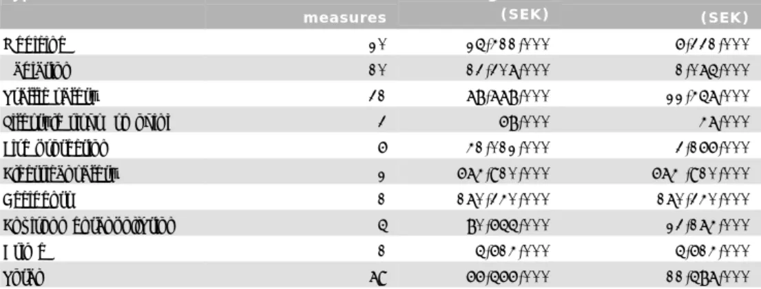
As shown in Table 1, the implicit cost per life saved is, on average, SEK 66.6 million, with a large variation among different sectors from SEK 68,000 to SEK 675 million. The median cost per life saved is approximately SEK 12 million. Rosén et al. (2006) compare the Swedish guideline values for contaminated sites to other risks and find that in some cases, 100-1,000 times higher health risks are accepted in working and housing environments compared to risks from contaminated sites.
From a societal perspective, a cost efficient allocation of resources occurs when the marginal cost of saving one life is equal in all interventions, given the same risk prefer-ences. If the marginal costs differ, resources should be reallocated to the sector with the lowest marginal costs. Departure from this principle implies that fever lives are saved at a given cost.5
The literature gives ample evidence on differences in the valuations of different types of risk reductions. Except socioeconomic factors, the character of the risk, the type of consequences, the baseline risk, and the magnitude of the risk reduction may also matter (Rosén et al., 2006). The public’s (and therefore the politicians’) risk percep-tions differ quite substantially from those of experts (Slovic et al., 1981; Chess et al., 2004). Differences in cost per life saved among different sectors can therefore partly be explained by differences in risk perceptions, even if very large differences can hardly be justified (Sjöberg, 2003).
5 Tengs and Graham (1996) show that it would be possible in the US to save an additional 60,000 lives per year
12
Table 1 The cost per life saved for primary prevention measures (SEK 2007 prices)
Type of measure Number of measures Average cost (SEK) Median cost (SEK) Medicine 20 25,411,000 6,331,000 Radiation 10 13,307,000 1,075,000 Traffic safety 31 78,778,000 22,457,000 Lifestyle risks (smoking) 3 68,000 47,000 Fire protection 6 41,012,000 3,166,000 Electrical safety 2 674,910,000 674 ,910,000 Accidents 1 170,340,000 170,340,000 Environmental pollution 5 80,655,000 23,174,000 Crime 1 5,614,000 5,614,000 Total 79 66,566,000 11,587,000
3.
Data
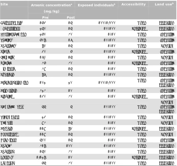
Of the 1,500 sites with highest priority, about 80 have been remediated or have on-going remediation financed by government funds. Even if a site has been nated by several pollutants, it is often possible to identify a so-called primary contami-nant. The primary contaminant is often the most hazardous and is present in the larg-est quantity, and hence guides the ambition level of the remediation work. Among the most prioritised sites metals (30 percent) and arsenic (26 percent) are the most com-mon primary contaminants (Swedish EPA, 2008b). Since metals can, in turn, be di-vided into mercury, lead, chromium, copper and cadmium, the single most common primary contaminant is arsenic which motivates the focus of the analysis. Table 2 lists the 23 arsenic-contaminated sites with either completed (10) or on-going measures (13).
Table 2 Site-specific characteristics
Arsenic concentrationa
(mg/kg) Site
Pre Post
Exposed individualsb Accessibility Land useb
Akterspegeln* 163 15 100-1,000 Open Recreation
Robertsfors 250 15 10-100 Enclosed Recreation Burträskbygden 260 40 1-10 Open Industry Tvärån* 608 17 10-100 Open Industry
Svartbyn* 80 15 1-10 Open Housing
Sjösa 30 6 10-100 Enclosed Industry
Lyshälla* 170 15 1-10 Open Housing
Mjölby 46 40 1-10 Enclosed Industry
Rimforsa 49 15 1-10 Open Industry Hjulsbro 87 15 10-100 Open Recreation
Glasbrukstomten 102 20 100-1,000 Open Industry Recreation Grimstorp 424 10 1-10 Open Industry
Elnaryd 130 40 1-10 Enclosed Industry Högsby–Ruda* 55 5 10-100 Open
Housing Industry Recreation
Tröingeberg 23 15 10-100 Open Housing Oxhult* 94 15 1-10 Open Housing
Gudarp 119 80 10-100 Enclosed Recreation Konsterud* 119 15 10-100 Open Housing
Kramfors* 500 15 1-10 Open Industry
Svanö* 418 100 10-100 Open Recreation
Svartvik 150 40 1-10 Open Recreation Forsmo* 1,128 10 1-10 Enclosed Recreation
Fagervik 65 40 10-100 Open Recreation
Note: Remediation has been completed (based on the quarterly report [Quarter 4, 2007] provided by the county administrative boards by order of the Swedish EPA). (a) The arsenic concentrations before remediation are derived from site-specific investigation reports or from involved consultants. (b) The land use data is derived from agent officials.
*
Arsenic contaminants result from previous industrial activities such as wood impreg-nation, and from sawmill, glasswork and sulphate and metal industries. Arsenic is mainly transported from contaminated sites through groundwater, but also through the air. Remediation work for arsenic is guided by health effects and not environ-mental effects (Swedish EPA, 2008c). Since there can be several risks involved, only
14
the primary risks need to be quantified (Swedish EPA, 2008d). Both acute health risks and long-term risks can be important for arsenic-contaminated sites. Arsenic is classi-fied as carcinogenic to humans (IARC, International Agency for Research on Cancer, 2004; 2008).6 That is, arsenic exposure is scientifically proven to increase the risk of developing cancer, primarily in the lungs, urinary bladder and skin, but probably also in the liver and kidneys (U.S. Department of Health and Human Services, US-HHS, 2007). At long-term low-level exposure to inorganic arsenic, cancer is the most impor-tant proven health risk, since blood vessel disease and skin changes (other than can-cer) do not occur below a certain exposure level.
ARSENIC CONCENTRATIONS
To estimate the risk reduction associated with arsenic mitigation, the average arsenic concentrations pre remediation have been collected. A reason for estimating risk based on an average concentration is that, over time, an individual will be exposed to an average concentration rather than to exceptionally high or low concentrations (US-EPA, 1992; Swedish EPA 2008d).7,8 As illustrated in Table 2, the average pre remedia-tion arsenic concentrations show a range from 23 to 1,128 mg/kg.9 The arsenic con-centrations post remediation refer to the sites’ quantitative remediation objectives. As illustrated in Table 2, a majority of the sampled sites have remediation objectives that correspond to the Swedish EPA’s guideline values for either sensitive, i.e. 15 mg/kg, or less sensitive, i.e. 40 mg/kg, land use. As shown, some of the sites’ remediation objec-tives have, however, been adjusted in regard to the site-specific background concen-trations of arsenic.
EXPOSURE
To be able to take actual exposure into account, we collected data from agent officials (i.e. municipality or county administrative board personnel) by asking them to ap-proximate the number of individuals on or adjacent to (i.e. within 500 metres of) a particular site. To simplify the approximation for the respondents, the following inter-vals were given: 1-10, 10-100 and 100-1,000. In addition, the respondents were asked to address the current and planned land use as well as the prevalence of children on or adjacent to the site. In order to take children who put fingers and occasionally soil in their mouth into account, we used the municipality’s share of children aged 0-3 years provided by Statistics Sweden.
6 The IARC is part of the World Health Organization. IARC is the publisher of the Monograph series
(1972-2002), which contains evaluations and classifications of environmental agents and exposures linked to the development of human cancer. The categories are: Group 1: Carcinogenic to humans ; Group 2A: Probably carcinogenic to humans ; Group 2B: Possibly carcinogenic to humans ; Group 3: Not classifiable as to carcinogenicity to humans ; and Group 4: Probably not carcinogenic to humans.
7 Commonly applied concentration values in risk assessments of contaminated sites are: average concentration;
Upper Confidence Limit (UCL) of the mean (based on t-statistics); a specific percentile (e.g. the 50th percentile
or the 95th percentile); and maximum measured concentration (Swedish EPA, 2008d).
8 A conservative average concentration (i.e. called UCL95) would, if available, be preferred (US-EPA, 2002;
Swedish EPA, 2008d) as the average site concentration depends on the depth and range of the investigated area, number of samples, purpose of sampling (i.e. to define the contaminated area or to determine the average concentration), and the distribution of concentrations (e.g. many samples with low concentrations and few with very high concentrations).
9 The natural background concentrations of arsenic vary. Depending on geographical location, concentrations from 3 to 15 mg/kg are found. Notably, for almost half of the sample sites the investigation reports do not provide information on background concentrations. Thus, these are not included in the subsequent quantifications.
Accessibility indicates whether a site is open or fenced. Land use refers to pre reme-diation use. The data onland use is relevant for approximating exposure times. The daily exposure times applied in subsequent quantifications (see the next section) is 24 hours for individuals residing on or adjacent to a site, 1 hour for recreational activities, and 5.7 hours for occupational activities. If pertinent, 5.7 hours also applies to day-care/school. We assume that both land use and the numbers of exposed individuals are unchanged post remediation, although it is plausible that both these factors in-crease post remediation. By assuming that these factors are unchanged we may hence underestimate the population at risk post remediation, overestimate the number of lives saved and, therefore, underestimate the cost per life saved.
16
4.
From exposure to lives saved
RISK ASSESSMENT
Since arsenic occurs naturally in the environment, humans are exposed by merely eating, drinking and breathing. The scientific task is to determine the levels of arsenic exposure and their effects on human health and the environment when additional con-taminant sources, like a contaminated site, are present. According to the MIFO risk assessment developed by the Swedish EPA, risk classification is based on an overall evaluation of the hazardousness and migration potential of site-specific contaminants, contamination level, and a site’s environmental sensitivity and protection value (Swed-ish EPA, 2007a). To be able to make lucid risk assessments of all contaminated sites, the Swedish EPA has compiled general guideline values for contaminants in the soil for different types of land use. The guideline values are in turn based on conservative assumptions about toxicological data and human exposure that often overestimate the risk posed by a site. These are national values and mark the levels that should not be exceeded. Occasionally, health risk assessments are supplemented with formal opin-ions from environmental medicine experts. In contrast to the conventional procedure for health risk assessment, environmental medicine personnel make use of their quali-fications in exposure assessment, toxicology and medicine to answer questions regard-ing e.g. what the actual exposure is at a specific site and what human health risks arise at a specific level of exposure.
The major aim of the Swedish EPA’s risk assessment is to compare site-specific con-taminant levels with the general guideline values. For health risk assessments, the starting point is, in general, the tolerable daily intake (TDI) that the World Health Organization (WHO) or other international organisations have recommended.10 For carcinogenic substances without thresholds, the general guideline value in Sweden is the value that is expected to result in one extra cancer case per 100,000 lifetime ex-posed individuals.11 It is then calculated how much an individual may actually be ex-posed to in total through aggregation of different exposure pathways at a certain con-taminant level. For sites with less sensitive land use (i.e. offices, industries, roads etc.), the exposure pathways are: direct intake of contaminated soil, dermal contact with contaminated soil and inhalation of dust from the contaminated site. For sites with sensitive land use (i.e. residential areas and playgrounds), all relevant exposure path-ways are considered (direct intake of soil, dermal contact, inhalation, intake of groundwater and intake of vegetables and fish). The Swedish EPA then makes stan-dardised assumptions and uses models to estimate dissemination from soil to air, drinking water, vegetables etc. (Swedish EPA, 1997, 2007b). Under the assumption that humans are exposed through all possible pathways (a so-called ‘worst case’), ex-posures through all pathways are added together. Then a general guideline value for the soil contaminant is calculated, which should protect humans from exceeding the TDI. The Swedish EPA does not make any judgment on the probability of exposure through a certain pathway. The precautionary principle is used for handling all uncer-tainties in the risk assessment, implying that in order to not underestimate the risks: (i) the contaminant levels should represent a ‘bad but possible scenario; (ii) possible but
10 The TDI is the amount of intake per kilo body weight per day of a chemical that can be ingested over a
lifetime without posing a significant risk to health.
11 This is a low risk to the individual. Since the lifetime risk of cancer in Sweden is around 40 percent, it implies
servative values should be chosen for the parameters in the risk assessment (Swedish EPA, 2007b).
Important to note is that the guideline values are national and that the risk is calcu-lated at the individual level. It does not matter how many individuals reside at or close to a contaminated site. The relation between the guideline value and the adverse effect is also unclear, which makes it difficult to relate a reduction in a contaminant level to a risk reduction (Rosén et al., 2006). To be able to make risk valuations, the risk before and after remediation needs to be quantified e.g. in the number of cancer cases avoided. Since the expected risk reduction is not quantified by the Swedish EPA, it is difficult to make socioeconomic priorities in remediation.
The model for generic guideline values can simplify the decision process in the early stages of risk assessment. One of the significant limitations is however that site-specific circumstances are only taken into account to a certain extent. The model is therefore indirect, mechanical and not directly applicable to calculate actual health risks. An environmental medicine assessment, on the other hand, aims to a larger ex-tent to assess the health risks associated with actual exposure. In such an analysis, the main exposure pathways are considered through toxicological methods. Exposure-response relationships from scientific studies are used to quantify health effects of different contaminants. An important difference between the two approaches is the time perspective. The Swedish EPA strives for long-term sustainability and argues that 100-1000 years should be considered. The environmental medicine approach strives to a larger extent to describe the actual exposure and does not usually analyse periods longer than a couple of decades (Liljelind and Barregård, 2008). Another difference is that environmental medicine treats high concentrations of contaminants on the sur-face more seriously than contaminants deeper down that humans normally do not risk being exposed to, except for the case of ingestion of ground water.
On a European level there are large differences between different models for guideline values. A comparison between European guideline value models is made by Carlon (2007) in order to analyse differences among methods and reasons behind these dif-ferences in order to identify possibilities for harmonisation. The difdif-ferences in some cases depend on sociocultural factors. In other cases the differences mirror different national strategies for environmental policies. Additionally, national differences can reflect lack of scientific consensus. In other cases there are no obvious reasons for the disparities and random factors seem to dominate, such as personal experience or his-torical aspects. For carcinogenic substances, the acceptable risk is expressed in extra cancer risk during a lifetime and varies between one per 10,000 and one per million in EU member states. The importance of this risk level should be evaluated in relation to the conservative assumptions made in the risk assessment, and then compared to the risks associated with other sources, such as air pollutants and smoking.
The consequences of exceeding guideline values vary according to national legislation. The strength in the execution of a sanction can also vary (Carlon, 2007). In the US, remediation started in the 1980s, and the focus has, as in Sweden, been placed on potential individual specific cancer risks rather than actual exposure. This has made the remediation programme much more expensive than planned. The annual cost of the US remediation programme ‘Superfund’ is now around USD 1,000 million. To
18
remediate the remaining sites is estimated to take 30 years and to cost USD 30,000 million in total (US EPA, 2004).
CALCULATING THE NUMBER OF CANCER CASES AVOIDED
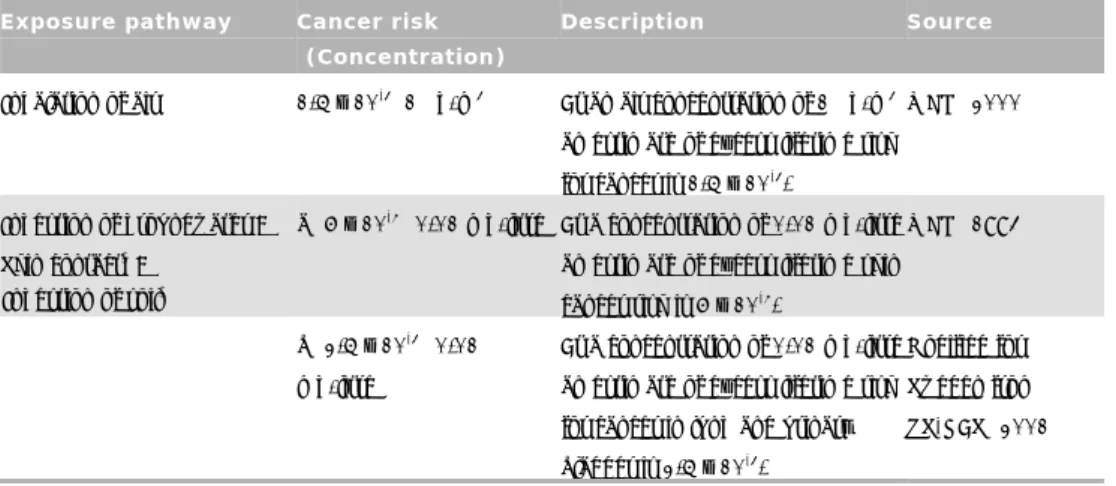
Exposure-response functions for different exposure pathways are used to calculate the extra cancer risk due to arsenic contamination. The main exposure pathways for can-cer risks due to arsenic-contaminated sites are: inhalation of air, ingestion of soil and skin contact.12 We depart from land use to estimate the exposure time for the site. The contaminant average concentration levels are then used to calculate the exposure for every pathway. For inhalation of air, the arsenic exposure is calculated based on as-sumptions of how the character of the soil affects the amount of particles in the air and that fine particles may contain higher concentrations of arsenic (see Appendix for an illustration). For ingestion of soil, the arsenic exposure is calculated based on as-sumptions of the amount of intake during the exposure time. For skin contact, the arsenic exposure is calculated based on assumptions of amount of soil on skin and percentage of skin absorption. These assumptions are all made in a manner that is customary for environmental medicine analyses. Uncertainties are indicated with an interval for certain factors (for example amount of soil on skin and bioavailability of arsenic contaminants). In the cases where such intervals are used, we have in the fol-lowing calculations used the values of the intervals that lead to the highest exposure, resulting in the highest possible numbers of lives saved.13 Hence, the calculations are conservative. If we instead would have used mid-interval estimates, the calculated risk and the number of saved cancer cases would have been several times lower. Thereaf-ter, exposure-response functions are applied to calculate the risk reduction caused by the remediation. Table 3 lists the exposure-response functions used in the calculations. First we calculate the number of cancer cases that may occur during a 30 year period if the site is not remediated. Then we calculate the risk that remains following remedia-tion, according to the Swedish EPA’s guideline values.14,15 The risk reduction there-fore consists of the difference between the risk pre remediation and the remaining risk post remediation. However, since not all cancer cases lead to death, the numbers must be adjusted when estimating the numbers of lives saved.16 The future cancer cases have not been discounted, since we do not know when in time they will occur.17 This implies that we underestimate the cost per life saved. It should be noted that we used a more updated risk assessment than the one used by the Swedish EPA. The number of cancer cases in our calculations becomes several times higher than if we had used the Swedish EPA’s exposure-response function. The reason is that not only do we take skin cancer into account, but also the risk for lung and bladder cancer.
12 In some cases the exposure-pathways ingestion of groundwater and intake of vegetables could be relevant.
Exposure through intake of vegetables has not been relevant for the sites included in this analysis. Exposure through ingestion of groundwater implies that the wells are used for drinkingwater and that the water contains contaminant levels that exceed drinkingwater guidelines for arsenic. There is risk for exposure through ingestion of groundwater on two of the sites. In addition there is risk for migration to groundwater on a third site. Our analysis is, however, limited to the exposure-pathways inhalation of air, ingestion of soil and skin contact.
13 That is, the numbers of exposed individuals are based on the upper bound of the applied intervals, and the
exposure times in regard to for instance residential activities are assumed to be as high as 24 h a day.
14 To use a 30 year period is consistent with the US EPA’s calculations (Viscusi, Hamilton and Dockins, 1997). 15 For more information about the data, see Forslund and Barregård (2008).
16 For lung cancer, mortality is more than 90 percent, but we have also calculated the risk for skin cancer and
bladder cancer, which have lower mortality (around 20 and 30 percent respectively). We therefore use 50 percent mortality in the calculations (see also Rosén et al., 2006, and Tallbäck et al., 2004).
Exposure pathway Cancer risk (Concentration)
Description Source
Inhalation of air 1.5 x 10⁻³ (1 μg/m3) At an air concentration of 1 μg/m3
an estimate of excess lifetime risk for cancer is 1.5 x 10⁻³.
WHO (2000)
Ingestion of groundwater ; Skin contact* ;
Ingestion of soil*
a) 6 x 10⁻⁴ (0.01 mg/litre) At a concentration of 0.01 mg/litre
an estimate of excess lifetime skin cancer risk is 6 x 10⁻⁴.
WHO (1993)
b) 2.5 x 10⁻³ (0.01
mg/litre)
At a concentration of 0.01 mg/litre an estimate of excess lifetime risk for cancer in lung and urinary bladder is 2.5 x 10⁻³.
Modified for Sweden from US-NAS (2001)
Note:* The Cancer risk was estimated assuming the same risk per unit of absorbed dose for exposure by
20
5.
The cost per life saved at arsenic sites
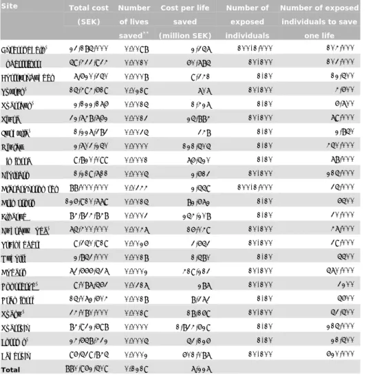
Table 4 shows that at most 0.03 lives will be saved through remediation of the site ‘Glasbrukstomten’. In total 0.12 lives can be expected to be saved on the arsenic sites at a cost of SEK 881 million. The cost per life saved on the arsenic sites varies from SEK 287 million to SEK 1,834,000 million. This widely exceeds the value of a statisti-cal life (VSL), which in Sweden is considered to be about SEK 21 million (SIKA, 2008). Even if we double the VSL, which has been suggested (SIKA, 2005) in order to take into account that valuations of reductions in risks of environmentally related mortality differ from valuations of reductions in risks of traffic related mortality, the difference is enormous. It is interesting to note that 72 percent of the health effects occur at three sites (Tvärån, Glasbrukstomten, Konsterud), where remediation costs amount to 13 percent of the total remediation costs. This underlines the importance of making the right priorities in the remediation work. The cost per life saved can be compared to similar estimates from an analysis of 150 contaminated sites financed by the US remediation program ‘Superfund’; there the average cost of an avoided cancer case amounted to USD 3 million (SEK 20 million), ranging from USD 20,000 (SEK 131,000) to USD 1,000 million (SEK 6,600,000 million) and with a median of USD 388 million (SEK 2553 million) (Hamilton and Viscusi, 1999), which can be compared to our average cost of one life saved of SEK 7,200 million and our median of SEK 16,000 million.18 The average Swedish cost is hence much higher than the U.S. average cost. If we are less conservative in our calculations on exposure, the cost per life saved becomes several times higher. We also calculated how many individuals need to be exposed at each site in order for one life to be saved. The results show that the num-ber of exposed must increase from 10-1,000 to 2,850-620,000 individuals. These fig-ures in some cases exceed the number of inhabitants in the municipality. Despite the uncertainties involved in our assumptions, the calculations illustrate that the ambition level in remediation is high, and in some cases unreasonably high.
18 The average cost is calculated as the quotient between the total remediation cost and the total number of
cancer cases avoided (or lives saved). If we instead use the average of the site-specific costs per cancer case avoided (or life saved), the average would be higher.
Table 4 Number of saved lives, costs and comparisons
Site Total cost (SEK)
Number of lives saved**
Cost per life saved (million SEK) Number of exposed individuals Number of exposed individuals to save one life Akterspegeln* 23,185,000 0.0098 2,357 100-1,000 104,000 Robertsfors 59,433,934 0.0010 60,785 10-100 103,000 Burträskbygden 7,620,350 0.0008 9,341 1-10 12,500 Tvärån* 15,494,619 0.0219 707 10-100 4,600 Svartbyn* 2,122,176 0.0015 1,427 1-10 6,700 Sjösa 32,748,762 0.0013 25,884 10-100 79,000 Lyshälla* 1,227,383 0.0035 348 1-10 2,850 Mjölby 2,703,250 0.0000 121,505 1-10 450,000 Rimforsa 9,820,099 0.0001 76,520 1-10 78,000 Hjulsbro 1,219,711 0.0005 2,613 10-100 215,000 Glasbrukstomten 88,000,000 0.0344 2,559 100-1,000 35,000 Grimstorp 126,910,779 0.0015 82,672 1-10 6500 Elnaryd 84,834,848 0.0003 254,208 1-10 30,000 Högsby–Ruda* 75,400,000 0.0047 16,049 10-100 47,000 Tröingeberg 9,350,919 0.0026 3,653 10-100 39,000 Oxhult* 2,853,000 0.0018 1,580 1-10 5500 Gudarp 73,666,537 0.0002 419,213 10-100 570,000 Konsterud* 9,087,563 0.0317 287 10-100 3200 Kramfors* 15,072,604 0.0018 8,373 1-10 5600 Svanö* 34,080,000 0.0019 18,169 10-100 53,500 Svartvik 84,932,698 0.0000 1,834,629 1-10 215,000 Forsmo* 24,658,432 0.0005 53,126 1-10 21,500 Fagervik 96,539,845 0.0002 601,087 10-100 620,000 Total 880,962,509 0.1219 7,227
Note: Indicates that remediation has been completed. For the sites with ongoing remediation the total cost is estimated. The cost is derived from the quarterly reports. Rounded to four decimals.
*
**
The analysis has not taken into account acute health risks, other health risks than can-cer and environmental risks. The acute risks are mostly associated with children’s pica-behaviour, i.e. the risk that children to a high extent put fingers and contaminated soil in their mouths. However, the risk that children eat soil at the arsenic-contaminated sites in our sample is considered to be very small. It is also questionable whether such small contributions to a human’s normal arsenic exposure are able to increase the risk of contracting any chronic disease other than cancer. The environmental risks differ among sites and are very difficult to estimate and value. As discussed earlier, it is the primary risks that should be valued, and in arsenic remediation health risks are consid-ered to be primary.
22
6.
Discussion
Remediation of contaminated sites is one of the most challenging Swedish environ-mental quality objectives in terms of reaching it on time. In addition, its cost amounts to as much as 10 percent of the total environmental budget. Sweden is only in the beginning of the remediation work, which until now has cost more than SEK 3,000 million, but is estimated to reach SEK 60,000 million after remediating the most haz-ardous sites. Internationally, the US Superfund has been criticised due to remediations having become much more expensive than estimated. In order for the Swedish objec-tives to be reached, remediation must prioritise the right sites and use an appropriate level of ambition.
Our results show that the level of ambition is high, maybe even too high. The cost per life saved under a 30 year period amounts to between SEK 287 million and
SEK 1,835,000 million in the 23 sites examined, despite conservative calculations that probably underestimate the cost. The average cost per life saved amounts to SEK 7,200 million. This widely exceeds the explicit value of a statistical life, which in Swe-den amounts to SEK 21 million (SIKA, 2008). Even if differences in risk preferences can motivate differences in marginal cost of saving lives, very large differences can hardly be justified. Based on our results we believe it is important to start a general discussion on how society’s resources should be spent in different sectors to save lives. What level of health risk is acceptable at contaminated sites, and how and why does this level differ from what is acceptable in terms of other health risk? Our results indicate that no more than 0.12 lives will be saved during a 30 year period at a cost of SEK 880 million. Compare this to the estimated 400 new lung cancer cases in Sweden each year (12,000 in 30 years) due to residential radon, and the several thousand pre-mature deaths every year due to air pollutants. If environmental health risks are to be reduced, there are probably other areas where economic resources can do more good. A societal decision criterion is that measures can be defensible as long as the benefit of the risk reduction is larger than the cost. The benefits consist mainly of reduced health and environmental risks. How come realistic quantifications of risk reductions at contaminated sites, which are a prerequisite for economic risk valuations, are so rare? While the Swedish EPA’s risk assessment starts from a guideline value and then assesses whether the contaminant concentrations exceed this value, it does not take actual exposure at the contaminated site into account. In Sweden, there is no estima-tion of a remediaestima-tion’s risk reducestima-tion and therefore no valuaestima-tion of the remediaestima-tion benefit. To be able to make risk valuations, a new working method is needed. Of course we believe it is important that Sweden decreases the pressure put on the envi-ronment, both nationally and globally. However, it is equally important that it is done in a manner that takes costs into account and weighs possible environmental benefits from different measures against each other. It simply seems reasonable to perform socioeconomic analyses when considering costly environmental policy measures.
Acknowledgements
The authors would like to thank Thomas Broberg,, Magnus Sjöström and Göran Öst-blom for useful comments, the Swedish EPA for providing us with data, and Mark Elert for valuable clarifications. Financial support from the Swedish Research Council for Environment, Agricultural Sciences and Spatial Planning (FORMAS) is gratefully acknowledged.
24
Appendix
Calculation of the extra cancer risk posed by arsenic-contaminated
air on the basis of soil concentration.
This exercise is based on the assumption that a site’s average arsenic concentration is 163 mg/kg. The site and its surroundings are used for recreational purposes and the number of individuals visit-ing the site is 100 per day.
Relevant parameters for approximating air exposure: (1) mass concentration of soil particles in inhaled air, (2) respirable particle fraction, and (3) exposure time (Swedish EPA, 1997).
The excess inhalable particle concentration tells how much of the total dust in the air that originates from the contaminated site. That is, the parameter depends on the soil characteristic (i.e. grass, sand, soil) and is assumed to vary from 1 to 5 µg/m3.
To control for the fact that fine particles in the air may contain higher concentrations than a sample of soil with a larger average particle size, a concentration factor of 1-5 is applied to the arsenic con-centration in soil.
The exposure time is based on land use. Approximating recreational activities to one hour a day, the population exposure is equivalent to a number of individuals exposed 24 hours/day given by
.
.
(1 h ÷ 24 h)×100 = 4 16 ≈4 individuals
Given the information above, the arsenic concentration in inhaled air can be calculated as:
.
.
.
.
.
3 3
1- 25 mg/m × 0 163 ng/mg = 0 163 - 4 075 ng/m
≈
0 16 - 4 1ng/m
3.As emphasised, the exposure-response function applied to quantify the number of cancer cases from air inhalation over a lifetime at or adjacent to the site is
1 5×10
.
-6 per ng/m3. The effect(cancer risk) is given by:
. . 3 . -6 3 . -6 . -6 -6
×10
References
Burström, K. (1999) Kostnadseffektivitetsstudier av primärpreventiva interventioner avseende hälsa (in Swedish), Socialmedicin 1999:6.
Carlon, C. (2007) Derivation methods of soil screening values in Europe. A review and evaluation of national procedures towards harmonisation.
Chess C, Hance BJ, Sandman PM. Bättre dialog med allmänheten. En kortfattad handledning för myndigheter I riskkommunikation (in Swedish). Universitetssjukhuset Örebro. Yrkes- och miljömed klin. Rapport R 92:1. Örebro 2004.
Forslund, J. and L. Barregård (2008) Remediation of sites contaminated by arsenic – Data to esti-mate the government cost for risk reduction, Brief Paper 2008:1, Konjunkturinstitutet. Gov. Bill 2000/01:130: Svenska miljömål – delmål och åtgärdsstrategier (in Swedish).
Gov. Bill 2004/05:150: Svenska miljömål – ett gemensamt uppdrag (in Swedish). Gov. Bill 2007/08:1: Budgetpropositionen för 2008” (in Swedish).
Hamilton, J. T. och W. K. Viscusi (1999) Calculating risks – The spatial and political dimensions of hazardous waste policy, The MIT Press, London, England.
Harvard Center for Cancer Prevention (1996), Harvard Report on Cancer Prevention, Cancer Causes and Control, 7.
IARC, International Agency for Research on Cancer (2004), “Some Drinking-water Disinfectants and Contaminants, including Arsenic – Summary of Data Reported and Evaluation”, IARC Monograpghs on the Evaluation of Carcinogenic Risks to Humans, Vol. 84.
IARC, International Agency for Research on Cancer (2008), “Overall Evaluations of Carcinogenicity to Humans”, Available at:
http://monographs.iarc.fr/ENG/Classification/crthgr01.php ; Accessed 2008-03-28.
Liljelind, I. and L. Barregård (2008) Hälsoriskbedömning vid utredning av förorenade områden (in Swedish), Report 5859, Swedish Environmental Protection Agency.
Ramsberg J. A. L. och L. Sjöberg (1997) The cost-effectiveness of life-saving interventions in Swe-den, Risk Analysis, Vol. 17, No 4.
Rosén L., R. Söderqvist, Å. Soutukorva, P.-E. Back, L. Grahn, H. Eklund (2006) ”Riskvärdering vid val av åtgärdsstrategi” (in Swedish), Report 5537, The Swedish Environmental Protection Agency.
SIKA (2005) Effektiva styrmedel för säkrare vägtrafik (in Swedish), SIKA PM 2005:8, Statens insti-tut för kommunikationsanalys, Stockholm.
SIKA (2008) Samhällsekonomiska principer och kalkylvärden för transportsektorn (in Swedish), SIKA PM 2008:3, Statens institut för kommunikationsanalys, Stockholm.
Sjöberg, L. (2003) Riskperception och attityder (in Swedish), Ekonomisk Debatt nr 6.
Slovic P., Fischhoff B. and Lichtenstein S. (1981): Perceived risk: Psychological factors and social implications. Proceedings of the Royal Society of London A376, 17-34.
Swedish EPA (1997), “Development of generic guideline values – model and data used for generic guideline values for contaminated soils in Sweden”, Rapport 4639, Naturvårdsverket. Swedish EPA, (2007a), “Environmental Quality Criteria for Contaminated sites”, Available at:
http://www.naturvardsverket.se/upload/english/03_state_of_environment/env_qual_criter ia/Contaminated_Sites.pdf, Accessed 2009-02-05.
Swedish EPA, The Swedish Environmental Protection Agency (2007b), “Rapport riskbedömning av förorenade områden – En vägledning från förenklad till fördjupad riskbedömning” (in Swedish), Remissversion 2007-10-19, Available at:
http://www.naturvardsverket.se/upload/30_global_meny/02_aktuellt/Remisser/vagledning smaterial_om_fororenade_omraden/Riskbedomning_av_fororenade_omraden_
26
Swedish EPA, The Swedish Environmental Protection Agency (2008a), “Lägesbeskrivning av ef-terbehandlingsarbetet i landet 2007” (in Swedish), Skrivelse, 2008-02-21, Dnr 642-516-08 Rf, Dnr 642-5732-07 Rf, Swedish EPA, Stockholm, Sweden.
Swedish EPA, The Swedish Environmental Protection Agency (2008b), “Lägesbeskrivning av ef-terbehandlingsarbetet i landet 2007 - Bilagor” (in Swedish), Skrivelse 2008-02-21, Swedish EPA, Stockholm, Sweden.
Swedish EPA, The Swedish Environmental Protection Agency (2008c), “Tabell över begränsande faktorer för riktvärdena för förorenad mark” (in Swedish), Available at:
http://www.naturvardsverket.se/sv/Verksamheter-med-miljopaverkan/Efterbehandling-av- fororenade-omraden/Riskbedomning/Nya-generella-riktvarden-for-fororenad-mark/Tabell-over-begransande-faktorer-for-riktvardena-for-fororenad-mark/ ; Accessed 2008-12-03. Swedish EPA, The Swedish Environmental Protection Agency (2008d), “Kostnads-nyttoanalys
som verktyg för prioritering av efterbehandlingsinsatser” (in Swedish), Naturvårdsverket, CM Gruppen AB, Stockholm, Sweden.
Tallbäck M, Rosén M, Stenbeck M, Dickman PW (2004). Cancer patient survival in Sweden at the beginning ot the third millennium – predictions using period analysis. Cancer Cause Contr 2004;15:967-976.
Tengs, T. och J. D. Graham (1996), ”The Opportunity Cost of Haphazard Social Investments in Life-Saving” i Hahn, R. W (red.), Risks, Costs and Lives Saved, Oxford University Press, New York.
US EPA (1992), Supplemental Guidance to RAGS: Calculating the Concentration Term. Publica-tion 9285.7-08I, Office of Solid Waste and Emergency Response, Hazardous Site EvaluaPublica-tion Division, Washington D.C.
US EPA (2002), “Calculating Upper Confidence Limits for Exposure Point Calculations at Haz-ardous Waste Sites”, Office of Emergency and Remedial Response, U.S. Environmental Pro-tection Agency, Washington D.C.
US EPA (2004), “Cleaning up the nation’s waste sites: markets and technology trends, EPA 542-R-04-015.
US-HHS, U.S. Department of Health and Human Services (2007), “Toxicological Profile for Arse-nic”, Public health Service, Agency for Toxic Substances and Disease Registry.
US-NAS, National Academy of Science, (2001), Arsenic in drinking water, 2001 update, National Academy Press, Washington DC:
Viscusi, K. W., J. T. Hamilton, P. C. Dockins (1997) “Conservative versus Mean Risk Assessments: Implications for Superfund Policies”, Journal of environmental economics and management 34, 187-206.
WHO, World Health Organization, (1993), ”Guideline for drinking-water quality 2nd Ed”, Volume 1, Geneva, Switzerland.
Titles in the Working Paper Series
No Author Title Year
1 Warne, Anders and Anders Vredin
Current Account and Business Cycles: Stylized Facts for Sweden
1989 2 Östblom, Göran Change in Technical Structure of the Swedish
Econ-omy
1989 3 Söderling, Paul Mamtax. A Dynamic CGE Model for Tax Reform
Simulations
1989 4 Kanis, Alfred and
Aleksander Markowski
The Supply Side of the Econometric Model of the NIER
1990 5 Berg, Lennart The Financial Sector in the SNEPQ Model 1991 6 Ågren, Anders and Bo
Jonsson
Consumer Attitudes, Buying Intentions and Con-sumption Expenditures. An Analysis of the Swedish Household Survey Data
1991 7 Berg, Lennart and
Reinhold Bergström
A Quarterly Consumption Function for Sweden 1979-1989
1991 8 Öller, Lars-Erik Good Business Cycle Forecasts- A Must for
Stabiliza-tion Policies
1992 9 Jonsson, Bo and
An-ders Ågren
Forecasting Car Expenditures Using Household Sur-vey Data
1992 10 Löfgren, Karl-Gustaf,
Bo Ranneby and Sara Sjöstedt
Forecasting the Business Cycle Not Using Minimum Autocorrelation Factors
1992 11 Gerlach, Stefan Current Quarter Forecasts of Swedish GNP Using
Monthly Variables
1992 12 Bergström, Reinhold The Relationship Between Manufacturing Production
and Different Business Survey Series in Sweden
1992 13 Edlund, Per-Olov and
Sune Karlsson
Forecasting the Swedish Unemployment Rate: VAR vs. Transfer Function Modelling
1992 14 Rahiala, Markku and
Timo Teräsvirta
Business Survey Data in Forecasting the Output of Swedish and Finnish Metal and Engineering Indus-tries: A Kalman Filter Approach
1992 15 Christofferson,
An-ders, Roland Roberts and Ulla Eriksson
The Relationship Between Manufacturing and Various BTS Series in Sweden Illuminated by Frequency and Complex Demodulate Methods
1992 16 Jonsson, Bo Sample Based Proportions as Values on an
Independ-ent Variable in a Regression Model
1992 17 Öller, Lars-Erik Eliciting Turning Point Warnings from Business
Sur-veys
1992 18 Forster, Margaret M Volatility, Trading Mechanisms and International
Cross-Listing
1992 19 Jonsson, Bo Prediction with a Linear Regression Model and Errors
in a Regressor
1992 20 Gorton, Gary and
Richard Rosen
Corporate Control, Portfolio Choice, and the Decline of Banking
1993 21 Gustafsson,
Claes-Håkan and Åke
The Index of Industrial Production – A Formal De-scription of the Process Behind it
28
Holmén
22 Karlsson, Tohmas A General Equilibrium Analysis of the Swedish Tax Reforms 1989-1991
1993 23 Jonsson, Bo Forecasting Car Expenditures Using Household
Sur-vey Data- A Comparison of Different Predictors
1993 24 Gennotte, Gerard and
Hayne Leland
Low Margins, Derivative Securitites and Volatility 1993 25 Boot, Arnoud W.A.
and Stuart I. Greenbaum
Discretion in the Regulation of U.S. Banking 1993 26 Spiegel, Matthew and
Deane J. Seppi
Does Round-the-Clock Trading Result in Pareto Im-provements?
1993 27 Seppi, Deane J. How Important are Block Trades in the Price
Discov-ery Process?
1993 28 Glosten, Lawrence R. Equilibrium in an Electronic Open Limit Order Book 1993 29 Boot, Arnoud W.A.,
Stuart I Greenbaum and Anjan V. Thakor
Reputation and Discretion in Financial Contracting 1993 30a Bergström, Reinhold The Full Tricotomous Scale Compared with Net
Bal-ances in Qualitative Business Survey Data – Experi-ences from the Swedish Business Tendency Surveys
1993 30b Bergström, Reinhold Quantitative Production Series Compared with
Qualiative Business Survey Series for Five Sectors of the Swedish Manufacturing Industry
1993 31 Lin, Chien-Fu Jeff and
Timo Teräsvirta
Testing the Constancy of Regression Parameters Against Continous Change
1993 32 Markowski,
Aleksan-der and Parameswar Nandakumar
A Long-Run Equilibrium Model for Sweden. The Theory Behind the Long-Run Solution to the Econometric Model KOSMOS
1993 33 Markowski,
Aleksan-der and Tony Persson
Capital Rental Cost and the Adjustment for the Ef-fects of the Investment Fund System in the Econo-metric Model Kosmos
1993 34 Kanis, Alfred and
Bharat Barot
On Determinants of Private Consumption in Sweden 1993 35 Kääntä, Pekka and
Christer Tallbom
Using Business Survey Data for Forecasting Swedish Quantitative Business Cycle Varable. A Kalman Filter Approach
1993 36 Ohlsson, Henry and
Anders Vredin
Political Cycles and Cyclical Policies. A New Test Approach Using Fiscal Forecasts
1993 37 Markowski,
Aleksan-der and Lars Ernsäter
The Supply Side in the Econometric Model KOS-MOS
1994 38 Gustafsson,
Claes-Håkan
On the Consistency of Data on Production, Deliver-ies, and Inventories in the Swedish Manufacturing Industry
1994 39 Rahiala, Markku and
Tapani Kovalainen
Modelling Wages Subject to Both Contracted Incre-ments and Drift by Means of a
Simultaneous-Equations Model with Non-Standard Error Structure
1994 40 Öller, Lars-Erik and
Christer Tallbom
Hybrid Indicators for the Swedish Economy Based on Noisy Statistical Data and the Business Tendency
41 Östblom, Göran A Converging Triangularization Algorithm and the Intertemporal Similarity of Production Structures
1994 42a Markowski,
Aleksan-der
Labour Supply, Hours Worked and Unemployment in the Econometric Model KOSMOS
1994 42b Markowski,
Aleksan-der
Wage Rate Determination in the Econometric Model KOSMOS
1994 43 Ahlroth, Sofia, Anders
Björklund and Anders Forslund
The Output of the Swedish Education Sector 1994 44a Markowski,
Aleksan-der
Private Consumption Expenditure in the Econometric Model KOSMOS
1994 44b Markowski,
Aleksan-der
The Input-Output Core: Determination of Inventory Investment and Other Business Output in the Econometric Model KOSMOS
1994 45 Bergström, Reinhold The Accuracy of the Swedish National Budget
Fore-casts 1955-92
1995 46 Sjöö, Boo Dynamic Adjustment and Long-Run Economic
Sta-bility
1995 47a Markowski,
Aleksan-der
Determination of the Effective Exchange Rate in the Econometric Model KOSMOS
1995 47b Markowski,
Aleksan-der
Interest Rate Determination in the Econometric Model KOSMOS
1995 48 Barot, Bharat Estimating the Effects of Wealth, Interest Rates and
Unemployment on Private Consumption in Sweden
1995 49 Lundvik, Petter Generational Accounting in a Small Open Economy 1996 50 Eriksson, Kimmo,
Johan Karlander and Lars-Erik Öller
Hierarchical Assignments: Stability and Fairness 1996 51 Url, Thomas Internationalists, Regionalists, or Eurocentrists 1996 52 Ruist, Erik Temporal Aggregation of an Econometric Equation 1996 53 Markowski,
Aleksan-der
The Financial Block in the Econometric Model KOSMOS
1996 54 Östblom, Göran Emissions to the Air and the Allocation of GDP:
Medium Term Projections for Sweden. In Conflict with the Goals of SO2, SO2 and NOX Emissions for
Year 2000
1996
55 Koskinen, Lasse, Aleksander Markows-ki, Parameswar Nan-dakumar and Lars-Erik Öller
Three Seminar Papers on Output Gap 1997
56 Oke, Timothy and Lars-Erik Öller
Testing for Short Memory in a VARMA Process 1997 57 Johansson, Anders
and Karl-Markus Mo-dén
Investment Plan Revisions and Share Price Volatility 1997 58 Lyhagen, Johan The Effect of Precautionary Saving on Consumption
in Sweden
1998 59 Koskinen, Lasse and A Hidden Markov Model as a Dynamic Bayesian 1998
30
Lars-Erik Öller Classifier, with an Application to Forecasting Busi-ness-Cycle Turning Points
60 Kragh, Börje and Aleksander Markowski
Kofi – a Macromodel of the Swedish Financial Mar-kets
1998 61 Gajda, Jan B. and
Aleksander Markowski
Model Evaluation Using Stochastic Simulations: The Case of the Econometric Model KOSMOS
1998 62 Johansson, Kerstin Exports in the Econometric Model KOSMOS 1998 63 Johansson, Kerstin Permanent Shocks and Spillovers: A Sectoral
Ap-proach Using a Structural VAR
1998 64 Öller, Lars-Erik and
Bharat Barot
Comparing the Accuracy of European GDP Forecasts 1999 65 Huhtala , Anni and
Eva Samakovlis
Does International Harmonization of Environmental Policy Instruments Make Economic Sense? The Case of Paper Recycling in Europe
1999 66 Nilsson, Charlotte A Unilateral Versus a Multilateral Carbon Dioxide Tax
- A Numerical Analysis With The European Model GEM-E3
1999 67 Braconier, Henrik and
Steinar Holden
The Public Budget Balance – Fiscal Indicators and Cyclical Sensitivity in the Nordic Countries
1999 68 Nilsson, Kristian Alternative Measures of the Swedish Real Exchange
Rate
1999 69 Östblom, Göran An Environmental Medium Term Economic Model –
EMEC
1999 70 Johnsson, Helena and
Peter Kaplan
An Econometric Study of Private Consumption Ex-penditure in Sweden
1999 71 Arai, Mahmood and
Fredrik Heyman
Permanent and Temporary Labour: Job and Worker Flows in Sweden 1989-1998
2000 72 Öller, Lars-Erik and
Bharat Barot
The Accuracy of European Growth and Inflation Forecasts
2000 73 Ahlroth, Sofia Correcting Net Domestic Product for Sulphur
Diox-ide and Nitrogen OxDiox-ide Emissions: Implementation of a Theoretical Model in Practice
2000 74 Andersson, Michael
K. And Mikael P. Gredenhoff
Improving Fractional Integration Tests with Boot-strap Distribution
2000 75 Nilsson, Charlotte and
Anni Huhtala
Is CO2 Trading Always Beneficial? A CGE-Model
Analysis on Secondary Environmental Benefits
2000 76 Skånberg, Kristian Constructing a Partially Environmentally Adjusted
Net Domestic Product for Sweden 1993 and 1997
2001 77 Huhtala, Anni, Annie
Toppinen and Mattias Boman,
An Environmental Accountant's Dilemma: Are Stumpage Prices Reliable Indicators of Resource Scar-city?
2001 78 Nilsson, Kristian Do Fundamentals Explain the Behavior of the Real
Effective Exchange Rate?
2002 79 Bharat, Barot Growth and Business Cycles for the Swedish
Econ-omy
2002 80 Bharat, Barot House Prices and Housing Investment in Sweden and
the United Kingdom. Econometric Analysis for the Period 1970-1998
2002 81 Hjelm, Göran Simultaneous Determination of NAIRU, Output 2003
dence 82 Huhtala, Anni and
Eva Samalkovis
Green Accounting, Air Pollution and Health 2003 83 Lindström, Tomas The Role of High-Tech Capital Formation for
Swed-ish Productivity Growth
2003 84 Hansson, Jesper, Per
Jansson and Mårten Löf
Business survey data: do they help in forecasting the macro economy?
2003 85 Boman, Mattias, Anni
Huhtala, Charlotte Nilsson, Sofia Ahl-roth, Göran Bostedt, Leif Mattson and Pei-chen Gong
Applying the Contingent Valuation Method in Re-source Accounting: A Bold Proposal
86 Gren, Ing-Marie Monetary Green Accounting and Ecosystem Services 2003 87 Samakovlis, Eva, Anni
Huhtala, Tom Bellan-der and Magnus Svar-tengren
Air Quality and Morbidity: Concentration-response Relationships for Sweden
2004
88 Alsterlind, Jan, Alek Markowski and Kristi-an Nilsson
Modelling the Foreign Sector in a Macroeconometric Model of Sweden
2004
89 Lindén, Johan The Labor Market in KIMOD 2004
90 Braconier, Henrik and Tomas Forsfält
A New Method for Constructing a Cyclically Adjusted Budget Balance: the Case of Sweden
2004 91 Hansen, Sten and
Tomas Lindström
Is Rising Returns to Scale a Figment of Poor Data? 2004 92 Hjelm, Göran When Are Fiscal Contractions Successful? Lessons for
Countries Within and Outside the EMU
2004 93 Östblom, Göran and
Samakovlis, Eva Costs of Climate Policy when Pollution Affects Health and Labour Productivity. A General Equilibrium Analysis Applied to Sweden
2004
94 Forslund Johanna, Eva Samakovlis and Maria Vredin Johans-son
Matters Risk? The Allocation of Government Subsi-dies for Remediation of Contaminated Sites under the Local Investment Programme
2006
95 Erlandsson Mattias and Alek Markowski
The Effective Exchange Rate Index KIX - Theory and Practice
2006 96 Östblom Göran and
Charlotte Berg
The EMEC model: Version 2.0 2006
97 Hammar, Henrik, Tommy Lundgren and Magnus Sjöström
The significance of transport costs in the Swedish forest industry
2006 98 Barot, Bharat Empirical Studies in Consumption, House Prices and
the Accuracy of European Growth and Inflation Forecasts
2006 99 Hjelm, Göran Kan arbetsmarknadens parter minska
jämviktsarbets-lösheten? Teori och modellsimuleringar
2006 100 Bergvall, Anders, To- KIMOD 1.0 Documentation of NIER´s Dynamic 2007