Anchor methods for DIF detection: A comparison
of the iterative forward, backward, constant and
all-other anchor class
Technical Report Number 141, 2013 Department of Statistics
University of Munich
of the iterative forward, backward, constant and
all-other anchor class
Julia Kopf Ludwig-Maximilians-Universit¨at M¨unchen Achim Zeileis Universit¨at Innsbruck Carolin Strobl Universit¨at Z¨urich Abstract
In the analysis of differential item functioning (DIF) using item response theory (IRT), a common metric is necessary to compare item parameters between groups of test-takers. In the Rasch model, the same restriction is placed on the item parameters in each group in order to define a common metric. However, the question how the items in the restriction – termed anchor items – are selected appropriately is still a major challenge. This article
proposes a conceptual framework for categorizing anchor methods: The anchor class
to describe characteristics of the anchor methods and the anchor selection strategy to
guide how the anchor items are determined. Furthermore, a new anchor class termed
the iterative forward anchor class is proposed. Several anchor classes are implemented
with two different anchor selection strategies (the all-other and the single-anchor selection strategy) and are compared in an extensive simulation study. The results show that the newly proposed anchor class combined with the single-anchor selection strategy is superior in situations where no prior knowledge about the direction of DIF is available. Moreover, it is shown that the proportion of DIF items in the anchor – rather than the fact whether
the anchor includes DIF items at all (termed contamination in previous studies) – is
crucial for suitable DIF analysis.
Keywords: Rasch model, anchoring, anchor selection, contamination, item response theory
1. Introduction
The analysis of differential item functioning (DIF) in item response theory (IRT) research investigates the violation of the invariant measurement property among subgroups of exami-nees, such as male and female test-takers. Invariant item parameters are necessary to assess ability differences between groups in an objective, fair way. If the invariance assumption is violated, different item characteristic curves occur in subgroups. In this paper, we focus on
uniform DIF where one group has a higher probability of solving an item (given the latent
trait) over the entire latent continuum and the group differences in the logit remain constant (Mellenbergh 1982;Swaminathan and Rogers 1990).
A variety of testing procedures for DIF on the item-level is available (e.g.,Lord 1980; Mellen-bergh 1982; Holland and Thayer 1988; Thissen, Steinberg, and Wainer 1988; Swaminathan and Rogers 1990;Shealy and Stout 1993, for an overview seeMillsap and Everson 1993). In the analysis of DIF using IRT, item parameters are to be compared across groups. Mostly, re-search focuses on the comparison of two pre-defined groups, the reference and the focal group. Thus, a common scale for both groups is required to assess meaningful differences in the item parameters. The minimum (necessary but not sufficient) requirement for the construction of a common scale in the Rasch model is to place the same restriction on the item parameters in both groups (Glas and Verhelst 1995). The items included in the restriction are termed
anchor items.
The anchor method determines how many items are used as anchor items and how they are located. Consistent with the literature, we use the term locate as a synonym for selecting anchor items. The choice of the anchor items has a high impact on the results of the DIF analysis: If the anchor includes one or more items with DIF, the anchor is referred to as
contaminated. In this case, the scales may be biased and items that are truly free of DIF
may appear to have DIF. Therefore, the false alarm rate may be seriously inflated – in the worst case all DIF-free items seem to display DIF (Wang 2004) – and the results of the DIF analysis are doubtful, as various examples demonstrate (see Section 2).
Even though the importance of the anchor method is undeniable, Lopez Rivas, Stark, and Chernyshenko (2009, p. 252) claim that “[a]t this point, little evidence is available to guide
applied researchers through the process of choosing anchor items”. Consequently, the aim of
this article is to provide guidelines how to choose an appropriate anchor for DIF analysis in the Rasch model.
In the interest of clarity, we introduce a new conceptual framework that distinguishes between
theanchor classand theanchor selection strategy. Firstly, theanchor class describes the
pre-specification of the anchor characteristics (such as a pre-defined anchor length). We review the all-other (used, e.g., by Cohen, Kim, and Wollack 1996; Kim and Cohen 1998), the constant anchor (used, e.g., by Thissen et al. 1988; Wang 2004; Shih and Wang 2009) and the iterative anchor class (referred to here as iterative backward and used, e.g., by Drasgow 1987; Candell and Drasgow 1988;Hidalgo-Montesinos and Lopez-Pina 2002). Furthermore, we introduce a new anchor class named the iterative forward anchor class. Secondly, the
anchor selection strategy determines which items are chosen as anchor items. We discuss the
all-other (introduced as rank-based strategy by Woods 2009) and the single-anchor selection strategy (proposed by Wang 2004). The complete procedure to choose the anchor is then called anchor method.
To derive guidelines which anchor method is appropriate for DIF detection in the Rasch model, we conduct an extensive simulation study. In our study, we compare the all-other, the constant, the iterative backward and the newly suggested iterative forward anchor class for
the first time. Furthermore, our study is to our knowledge the first to systematically contrast different anchor selection strategies that are combined with the anchor classes mentioned above. Altogether, nine different anchor methods are evaluated regarding their appropriate-ness for DIF analysis. Finally, practical recommendations are given to facilitate the process of selecting anchor items for DIF analysis in the Rasch model.
In the next section, technical details of the anchor process for the Rasch model are explained and illustrated by means of an instructive example and the framework of anchor classes, an-chor selection strategies and anan-chor methods is introduced in detail. The simulation study is presented in Section3 and the results are discussed in Section4. The problem of contamina-tion and its impact on DIF analysis are addressed in Seccontamina-tion5. Characteristics of the selected anchor items are discussed in Section 6. A concluding summary of the simulation results and practical recommendations are given in Section 7.
2. A conceptual framework for anchor methods
In the following, the anchor process is technically described and analyzed for the Rasch model. The item parameter vector is β = (β1, . . . , βk)>∈Rk, where k denotes the number of items
in the test. In the following, it is estimated using the conditional maximum likelihood (CML) estimation due to its unique statistical properties, its widespread application (Wang 2004) and the fact that its estimation process does not rely on the person parameters (Molenaar 1995).
As the origin of the scale in the Rasch model can be arbitrarily chosen (Fischer 1995) – what is often referred to as scale indeterminacy – one linear restriction of the form
k
X
`=1
a`β˜`= 0, (1)
with constants a` holding Pk`=1a` 6= 0 is placed on the item parameter estimates ˜β` (Eggen
and Verhelst 2006). Thus, in the Rasch model onlyk−1 parameters are free to vary and one parameter is determined by the restriction. Note that equation 1includes various commonly used restrictions such as setting one item parameter ˜β`= 0 or restricting all item parameters
to sum zeroPk`=1β˜`= 0 (Eggen and Verhelst 2006). Without loss of generality, we here
esti-mate the item parameter vector ˜β with the employed restriction ˜β1 = 0. The corresponding
covariance matrix dVar( ˜β) then contains zero entries in the first row and in the first column. It is irrelevant which particular restriction is chosen to identify the parameters, as the in-terpretation of the results is independent of the restriction employed. In the following, we discuss different restrictions for which the sum of a selection of items is set to zero andais an indicator vector. These restrictions can be obtained by transformation using the equations
ˆ
β = Aβ˜ (2)
and Var( ˆd β) = AVar( ˜d β)A>, (3) whereA=Ik−Pk1
`=1a`1k·a
>,I
kdenotes the identity matrix, 1kdenotes a vector of one entries
andais a vector with one entries for those elementsa`that are included in the restriction and
zero entries otherwise (e.g., a= (1,0,1,0,0, . . .)> including item 1 and item 3). Additionally, the entries of the rank deficient covariance matrix Var( ˆd β) in the row and in the column of the item that is first included in the restriction are set to zero.
While for the estimation itself, the choice of the restriction is arbitrary, for the anchor process a careful consideration of the linear restriction that is now employed in each group g is necessary. A necessary but not sufficient requirement in order to build a common scale for two groups is that the same restriction is employed in both groups (Glas and Verhelst 1995). Items in the restriction are termed anchor items and the restriction can be rewritten as
k X `=1 a`βˆ`g = X `∈A ˆ β`g = 0, (4)
where the setAis termed theset of anchor itemsor theanchor. The estimated and anchored item parameters are denoted ˆβg. Equation4includes various commonly used anchor methods such as setting one item parameter ˆβg` to zero ( ˆβ`g = 0, for one ` ∈ {1,2, . . . , k}) for the so called constant single-anchor method or restricting all items except the studied item j to sum zero in each group (P`6=jβˆ`g = 0) for the so called all-other anchor method. The item parameters, estimated separately in each group, are transformed to the respective anchor method by using equation 2, where all items are then shifted on the scale by− 1
|A|
P
`∈Aβ˜
g
`.
The covariance matrices are transformed using equation 3.
Furthermore, the anchor items should be DIF-free. Otherwise, if for example the single anchor item that is restricted to zero in both groups is a DIF item, the construction of a common scale fails as all other items are artificially shifted apart as will be shown in the following example (for a detailed illustration see also Wang 2004). This is termed artificial DIF by Andrich and Hagquist(2012). Unfortunately, since prior to DIF analysis it cannot be known which items are DIF-free, we face a somewhat circular problem, as pointed out by Shih and Wang (2009).
The construction of a common scale is now illustrated by means of an instructive example. The data set from a general knowledge quiz was conducted by the weekly German news magazine SPIEGEL in 2009. A thorough discussion and analysis of the original data set are provided in Trepte and Verbeet(2010) including a global DIF analysis by means of model-based recursive partitioning byStrobl, Kopf, and Zeileis(2010). From about 700,000 test-takers that answered each a total of 45 items from different domains, we select a subsample of 9,442 test-takers (that obtained their A-levels in Germany) and four items from politics (listed below together with the correct answers) for the illustration of the anchor problem:
Item 1 Who determines the rules of action in politics according to the German Constitution? (The Bundeskanzler.)
Item 2 What is the role of the second vote in the elections for the German Bundestag? (It governs the seating in the German Bundestag.)
Item 3 How many people were killed by the RAF? (33) Item 4 Indicate the location of Hessen on the German map.
As an exemplary illustration, let us suppose we want to test for DIF in the first item between the focal (foc) group of the test-takers that obtained their A-levels in the German federal state Hessen and the reference (ref) group of all remaining test-takers.
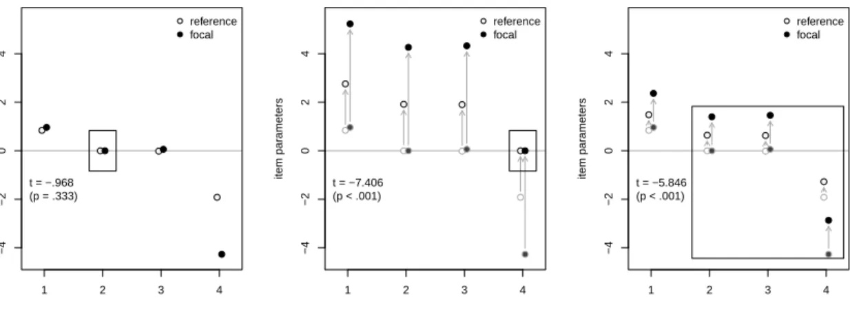
Figure 1 displays three different restrictions: The second item as constant single-anchor, the fourth item as constant single-anchor and all other items (item 2 to item 4) as anchor. The points represent the estimated item parameters from the reference (light points) and the focal group (dark points). The rectangles surround the anchor item(s).
In Figure 1 (left), item 2 is used as constant single-anchor and, thus, both estimated item parameters are set to zero. The results here display the estimated item parameters. The negligible difference in the item parameters of item 1, that we are currently interested in,
suggests no DIF in this item. To understand the DIF test results for item 1 in the next scenarios, it is also important to note that the large difference in item 4 implies DIF in this item. Since item 4 was the question to indicate the location of Hessen on the German map, it is plausible that this item 4 is a true DIF item since it was easier for test-takers that obtained their A-levels in Hessen. The item-wise Wald test (see Lord 1980 and equation 5 below) for item 1 does not display statistically significant DIF (t=−.968 with the corresponding p-value of .333). As a result, item 1 is classified as DIF-free.
item 2 as constant single−anchor
item par ameters ● ● ● ● ● ● ● ● 1 2 3 4 −4 −2 0 2 4 ● ● reference focal t = −.968 (p = .333)
item 4 as constant single−anchor
item par ameters ● ● ● ● ● ● ● ● ● ● ● ● ● ● ● ● 1 2 3 4 −4 −2 0 2 4 ● ● reference focal t = −7.406 (p < .001)
all other items as anchor
item par ameters ● ● ● ● ● ● ● ● ● ● ● ● ● ● ● ● 1 2 3 4 −4 −2 0 2 4 ● ● reference focal t = −5.846 (p < .001)
Figure 1: Different restrictions placed on the item parameters that are estimated using the Rasch model in each group.
In the next scenario in Figure 1 (middle), the (suspected) DIF item 4 is used as a constant single-anchor. Compared to the first scenario, the item parameters are now shifted upwards by the estimated difficulties of item 4 (approximately 2 for the reference and 4 for the focal group as indicated by the arrows). The difference that now occurs for item 1, that we are currently interested in, is likely to reflect the presence of artificial DIF. Here, the statistical test indicates DIF for item 1 (t = −7.406 with the corresponding p-value < .001). Hence, item 1 is classified as a DIF item.
In the last scenario in Figure 1 (right), all other items – except the currently studied item 1 – are used as anchor items. Compared to the first scenario where item 2 was set to zero, all items are shifted upwards by the average over the estimated difficulties of item 2, 3 and 4. Now, all item parameters are shifted apart. Compared to the second scenario, the scales are shifted apart less strongly since the scale shift is reduced from the estimated difficulties of the suspected DIF item 4 to the average over the estimated difficulties of item 2, 3 and 4 (including the presumed DIF-free items 2 and 3) as visible by the shorter arrows. However, the statistical test still classifies item 1 as a DIF item (t = −5.846 with the corresponding p-value < .001). This example illustrates the major impact of the anchor method on the results of the DIF analysis, since – depending on the anchor set – three different test statistics result in the DIF tests for item 1.
From a theoretical perspective and from our instructive example, it is obvious that an appro-priate anchor is crucial for the results of the DIF analysis. Previous simulation studies have compared different selections of anchor methods (an overview over the existing literature will be given in Section 3.4). Empirical findings also show that, ideally, the anchor items should
be DIF-free. Otherwise, thecontamination may lead to seriously augmented false alarm rates in DIF detection (see, e.g.,Wang and Yeh 2003;Wang 2004;Wang and Su 2004;Finch 2005; Stark, Chernyshenko, and Drasgow 2006;Woods 2009) that “can result in the inefficient use
of testing resources, and [...] may interfere with the study of the underlying causes of DIF”
(Jodoin and Gierl 2001, p. 329). Naturally, the risk of contamination would suggest to use only few items in the restriction (i.e. a short anchor), but the simulation results also show that the statistical power increases with the length of a DIF-free anchor (Thissenet al.1988; Wang and Yeh 2003;Wang 2004;Shih and Wang 2009;Woods 2009).
Therefore, in the following this trade-off between the false alarm rate (DIF-free items that are erroneously diagnosed with DIF) and the hit rate (DIF items that are correctly diagnosed with DIF) is analyzed for different anchor methods in a simulation study. As a statistical test for DIF we will focus on the item-wise Wald test here (Lord 1980). For the Wald test, the item parameters are first estimated separately in each group. The anchor methods are then used to obtain a common scale for the item parameters which are to be compared.
The rationale behind the Wald test is that DIF is present if the item difficulties are not equal across groups. The test statistic Tj for the null hypothesis H0 :βjref = βjfoc, where βjref and βjfoc denote the item difficulties for reference and focal group for itemj and ˆβjref and ˆβjfoc the corresponding estimated item parameters using the anchor Aj, has the following form:
Tj = ˆ βjref−βˆjfoc q d Var( ˆβref j −βˆjfoc) = ˆ βjref−βˆjfoc q d Var( ˆβref) j,j+Var( ˆd βfoc)j,j . (5)
Note that, the estimated and anchored item parameters ˆβ = ˆβ(Aj), which can be calculated
using equation 2, depend on the anchor and, hence, so does the test statistic Tj = Tj(Aj).
The anchor setAj may depend on the studied item (as is the case for the all-other method). If the anchor is constant regardless which item is tested for DIF, it is denotedAin the following. 2.1. Anchor classes
In our conceptual frameworkanchor classesdescribe characteristics of the anchor that answer the following questions: Is the anchor length pre-defined? If so, how many items are included in the anchor? Is the anchor determined by the anchor class itself or is an additional anchor selection strategy necessary? Are iterative steps intended to define the anchor?
In theequal-mean-difficulty anchor class (see, e.g.,Wang 2004, and the references therein) all items are restricted to have the same mean difficulty (typically zero) in both groups, whereas in theall-other anchor class the sum of all items – except the item currently tested for DIF – is restricted to be zero. Both anchor classes have a pre-defined anchor length but no additional anchor selection is necessary as the items included in the restriction are already determined by the anchor class itself. The equal-mean-difficulty and the all-other class only differ in one anchor item and, therefore, essentially lead to similar results (cf.Wang 2004). Since it seems reasonable not to include the item currently tested for DIF in the anchor, only the all-other method is included in the following simulation study.
The constant anchor class includes a pre-defined number of the test items (e.g., 1 or 4 items
according to Thissen et al.1988) or a certain proportion of the test items (e.g., 10% or 20% according to Woods 2009) as anchor. The term constant reflects the pre-defined, constant anchor length. In our simulation study, we implemented the constant anchor class with one single anchor item as well as the constant anchor including four items, which is supposed
to assure sufficient power (cf. e.g., Shih and Wang 2009; Wang, Shih, and Sun 2012). The constant anchor class needs to be combined with an explicit anchor selection strategy.
The iterative backward anchor class includes a variety of iterative methods that have been
suggested, discussed and combined with different statistical methods to assess DIF. Here, we focus on the commonly used re-linking procedure where one parameter estimation step suffices to conduct DIF analysis. Firstly, the scales of both groups are linked on (approximately) the same metric, e.g., by using the all-other anchor method. Then, the DIF items are excluded from the current anchor, the scales are re-linked using the new current anchor, the DIF analysis is carried out and the steps are repeated until two steps reach the same results (e.g., Drasgow 1987; Candell and Drasgow 1988; Park and Lautenschlager 1990; Kim and Cohen 1995;Hidalgo-Montesinos and Lopez-Pina 2002). This iterative procedure is referred to here as the iterative backward anchor class, since the method includes the majority of items in the anchor at the beginning. Then, it successively excludes items from the anchor.
The research of Wang and Yeh(2003),Wang(2004), Shih and Wang(2009) and Wanget al.
(2012) made clear that the direction of DIF influences the results of the DIF analysis using all other items as anchor: If all items favor one group, DIF tests using all other items as anchor perform weak. Hence, in complex DIF situations such as unbalanced DIF, the initial step of the iterative-backward anchor class, that includes all other items as anchor, may lead to biased test results.
Inspired by the results of Wang and Yeh (2003), Wang (2004), Shih and Wang (2009) and Wang et al. (2012), we introduce another possible strategy to overcome the problem that the anchor selection is based on initially biased test results: The iterative forward anchor class. As opposed to the iterative backward class, we suggest to build the iterative anchor in a step-by-step forward procedure. Starting with one single anchor item, we link the scales and estimate DIF. Then, iteratively, as long as the current anchor length is shorter than the number of currently presumed DIF-free items, one item – located by means of the respective anchor selection strategy – is added to the current anchor and DIF analysis is conducted using the new current anchor. Unlike the iterative backward anchor class where items are successively excluded, now items are successively included in the anchor. An anchor selection strategy is again needed to guide which items are included in the anchor.
The rationale behind the iterative forward approach is similar to the common approach in confirmatory factor analysis (CFA) described by Starket al. (2006), where one referent item is constrained to conduct DIF analysis. Here, we determine an order of candidate anchor items and guide the decision whether additional anchor items are included by DIF tests for all items (except the first anchor item, see Section 2.3) using the current anchor.
2.2. Anchor selection strategies
The anchor selection strategies discussed here are based on preliminary item analyses. This means that DIF tests are conducted to locate – ideally – DIF-free anchor items. The (non-statistical) alternative relying on expert advice and certain prior knowledge of DIF-free anchor items (Wang 2004;Woods 2009) will not often be possible in practice (for a literature overview where this approach fails see Frederickx, Tuerlinckx, De Boeck, and Magis 2010).
In our simulation study, we implemented different anchor selection strategies that provide a ranking order of candidate anchor items. One anchor selection strategy investigated in this article is the rank-based strategy proposed by Woods (2009) that we term all-other (AO) anchor selection strategy. Initially, every item j = 1, . . . , k is tested for DIF using all other items as anchor. This implies an anchor set Aj ={1, . . . , k} \j that depends on the studied
item j. The anchor is then chosen according to the lowest rank(s) of the resulting (absolute) DIF test statistics.
A selection strategy proposed by Wang(2004) – applied in a modified version for the MIMIC procedure byShih and Wang(2009) – is called single-anchor (SA) selection strategy here and, to our knowledge, for the first time systematically compared with the all-other strategy using various anchor classes. With every item acting as single-anchor, every other item is tested for DIF. Again, the anchor setsAj vary across the studied items and k−1 tests result for every
item j = 1, . . . , k of the test. The anchor is then chosen from the items with the smallest
number of significant results. If more than one item displays the same number of significant results, one of the corresponding items is selected randomly. A similar approach was suggested by Cheung and Rensvold(1999) in the context of factorial invariance to concurrently select a set of non-variant items that also relies on results testing every item by using every other item in the restriction.
2.3. Anchor methods
An anchor method results as a combination of an anchor class with an anchor selection
strategy (in cases where the latter is necessary). The anchor methods to be investigated in this article are now presented with details of the implementation and summarized in Table1. The all-other anchor method (all-other) does not require an additional anchor selection. Every item is tested for DIF using all remaining items as anchor items. Here, the anchor set
Aj = {1, . . . , k} \j depends on the studied item j = 1, . . . , k and one re-linking step is
necessary for each item.
All remaining anchor methods consist of two steps: Firstly, the anchor selection is carried out to determine a ranking order of candidate anchor items and the proceeding of the anchor class is carried out to determine the final anchor. Secondly, the final anchor found in the first step is then used for the assessment of DIF. This procedure was termed DIF-free-then-DIF strategy by Wang et al. (2012). For the following anchor methods, the final anchor A is independent of which item is studied. Since k−1 parameters are free in the estimation, only
k−1 estimated standard errors result (Molenaar 1995), the k-th standard error is determined by the restriction and, hence, only k−1 tests can be carried out and one item in the final assessment of DIF obtains no DIF test statistic. Thus, for the following anchor methods, the first item selected as anchor item is presumed DIF-free in the final DIF test and all remaining test items are tested for DIF using the final anchor A.
The constant anchor class consisting of one anchor item or four anchor items can be combined with the all-other selection strategy (single-anchor-AO, four-anchor-AO). The anchor is se-lected according to the lowest rank(s) of the DIF test statistics resulting from the initial DIF tests for every item using the all-other method (Woods 2009). The final DIF test is conducted after re-linking the parameters using the final anchor.
The constant anchor class can also be combined with the single-anchor selection strategy
(single-anchor-SA, four-anchor-SA). In this case, initially every item is tested for DIF by
using every other item as single-anchor. The final anchor (consisting of either one item for the single-anchor-SA or four items for the four-anchor-SA method) is selected from the set of items displaying the smallest number of significant test results.
Furthermore, we implemented a suggestion ofWang(2004) that we refer to as the four-anchor next candidate (NC) method. In the four-anchor-NC method, the item that is selected by the SA-selection strategy functions as the current single-anchor and DIF tests are conducted (see Wang 2004, p. 249) similar to the single-anchor-SA method. In this step, one DIF test
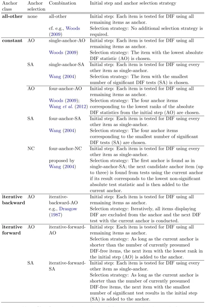
Anchor class
Anchor selection
Combination Initial step and anchor selection strategy
all-other none all-other Initial step: Each item is tested for DIF using all
remaining items as anchor. cf. e.g., Woods
(2009)
Selection strategy: No additional selection strategy is required.
constant AO single-anchor-AO Initial step: Each item is tested for DIF using all
remaining items as anchor.
Woods (2009) Selection strategy: The item with the lowest absolute DIF statistic (AO) is chosen.
SA single-anchor-SA Initial step: Each item is tested for DIF using every other item as single-anchor.
Wang (2004) Selection strategy: The item with the smallest number of significant DIF tests (SA) is chosen. AO four-anchor-AO Initial step: Each item is tested for DIF using all
remaining items as anchor. Woods (2009);
Wanget al.(2012)
Selection strategy: The four anchor items
corresponding to the lowest ranks of the absolute DIF statistics from the initial step (AO) are chosen. SA four-anchor-SA Initial step: Each item is tested for DIF using every
other item as single-anchor.
Wang (2004) Selection strategy: The four anchor items
corresponding to the smallest number of significant DIF tests (SA) are chosen.
NC four-anchor-NC Initial step: Each item is tested for DIF using every other item as single-anchor.
proposed by Wang (2004)
Selection strategy: The first anchor is found as in single-anchor-SA; the next candidate anchor item (up to three) is found from tests using the current anchor if its result corresponds to the lowest non-significant absolute test statistic and is then added to the current anchor.
iterative backward
AO iterative-backward-AO
Initial step: Each item is tested for DIF using all remaining items as anchor.
e.g., Drasgow (1987)
Selection strategy: Iteratively, all items displaying DIF are excluded from the anchor and the next DIF test with the current anchor is conducted.
iterative forward
AO iterative-forward-AO
Initial step: Each item is tested for DIF using all remaining items as anchor.
Selection strategy: As long as the current anchor is shorter than the number of currently presumed DIF-free items, the next item with the lowest rank in the initial step (AO) is added to the anchor.
SA iterative-forward-SA
Initial step: Each item is tested for DIF using every other item as single-anchor.
Selection strategy: As long as the current anchor is shorter than the number of currently presumed DIF-free items, the next item with the smallest number of significant test results in the initial step (SA) is added to the anchor.
statistic results for every item except for the anchor. The next candidate anchor item is the item that displays “the least magnitude of DIF” (Wang 2004, p. 250) among all remaining items that we defined as lowest absolute DIF test statistic from the tests using the current single-anchor item. The candidate item is added to the current anchor only if its DIF test result is not significant (Wang 2004).1 The next DIF test is conducted using the new current anchor and the next candidate item is selected again if it has the lowest absolute DIF test statistic among all remaining items and displays no significant DIF. These steps are repeated until either the next candidate anchor item displays DIF or the maximum anchor length (of four items in our implementation) is reached.
Technically speaking, this procedure is a combination of the constant and the iterative anchor class because it allows a varying anchor length but its length is limited to a pre-specified number of items. However, since in our simulation always four anchor items were selected for the final anchor, here we classify the anchor class as constant.
The iterative backward class is implemented using all-other items as anchor in the initial step and then excluding DIF items from the anchor (iterative-backward-AO) as it is widely used in practice (e.g., Bolt, Hare, Vitale, and Newman 2004; Edelen, Thissen, Teresi, Kleinman, and Ocepek-Welikson 2006). When items are excluded from the anchor, the scales are re-linked with the new current anchor and DIF tests are conducted. Items displaying DIF are again excluded from the anchor and the steps are repeated until the final anchor is found.2 Note that the iterative backward class is not combined with the SA-selection since the latter provides only a ranking order of candidate anchor items, but no information which set of items should be used in the initial step.
The newly suggested iterative forward class can be combined with the all-other anchor selec-tion strategy (iterative-forward-AO). In this case, DIF analysis for every item is conducted using the all-other method. The DIF test statistics are again ranked by their absolute value. The item corresponding to the lowest DIF test statistic is the first anchor item. As long as the anchor length does not exceed the number of currently presumed DIF-free items, the item with the next lowest absolute DIF test statistic from the initial step is included in the current anchor and DIF analysis is carried out using the new current anchor to check whether the anchor length exceeds the number of presumed DIF-free items. When the final iteration is reached, again, DIF analysis is conducted with the new final anchor, where, again, the first anchor item is presumed DIF-free.
Furthermore, the proposed iterative forward class can be also combined with the single-anchor selection strategy (iterative-forward-SA). In this case, initially every item is tested for DIF using every other item as single-anchor. The items are ranked according to the number of significant test results. The item with the smallest number of significant test results is chosen as anchor. As long as the anchor length does not exceed the number of currently presumed DIF-free items, the next (new) item displaying the smallest number of significant DIF tests from the initial step is included in the anchor and DIF analysis is carried out using the new current anchor to check whether the current anchor length exceeds the number of currently presumed DIF-free items. When the final iteration is reached, the DIF test results of the DIF analysis using the final anchor are returned and the first anchor item is presumed DIF-free.
1We employed a significance level of.05, but future research may investigate the additional proposition of
Wang(2004) augmenting it to e.g.,.30.
2In case all items were excluded from the anchor (which happened in only 2 out of 154,000 replications),
3. Simulation study
To evaluate which of the anchor methods presented in the previous section (for a brief descrip-tion and nomenclature see again Table 1) are best suited to correctly classify items with and without DIF, an extensive simulation study is conducted. 2000 data sets are generated from each of 77 different simulation settings. For every data set, the item-wise Wald test (Lord 1980, see Section2) – based on the currently investigated anchor method – is conducted at the significance level of .05 in the free R system for statistical computing (R Development Core Team 2011). A short description of the study design is given in the following paragraphs. Parts of the simulation design were inspired by the settings used byWoods(2009) andWang (2004).
3.1. Data generating process
Each data set, that represents one of 2000 replications from one simulation setting, corre-sponds to the simulated responses of two groups of subjects (thereference (ref) and thefocal
(foc) group) in a test with k= 40 items.
• Person and item parameters
The person parameters are generated from a normal ability distribution with a higher mean for the reference group θref ∼N(0.5,1) than for the focal group θfoc ∼N(0,1). Values assigned to the item parameters are replicated from the sequence of βjref ∈ {−1,−0.5,0,0.5,1} in equal proportions.
• DIF items
In case of DIF, the affected DIF items are chosen randomly to display uniform DIF by setting the difference in the item parameters of reference and focal group ∆DIF = βjref−βjfoc to +.5 or−.5 (consistent with the intended direction of DIF).
• IRT model
The responses in each group follow the Rasch model. They are generated in two steps: The probability of person i solving item j is computed by placing the corresponding item and person parameters in the Rasch model formula 6. The binary responses are then drawn from a binomial distribution with the resulting probabilities.
P(Uij = 1|θi, βj) =
exp(θi−βj)
1 + exp(θi−βj)
(6)
3.2. Manipulated variables
Three main conditions determine the specification of the manipulated variables: One condition under the null hypothesis where no DIF is present and two conditions under the alternative where DIF is present.
• Sample sizes
The sample sizes in reference and focal group are defined by the following pairs (nref, nfoc)
∈ {(250,250), (500,250), (500,500), (750,500), (750,750),. . ., (1500,1500)}. Thus, both equal and different group sizes are considered.
• Directions and proportions of DIF
Under the condition of the null hypothesis (no DIF), only the sample sizes are varied. The two remaining conditions represent the alternative hypothesis where DIF is present, but they differ with respect to the direction of DIF: The second condition represents
balanced DIF. Here, each DIF item favors either the reference or the focal group but
no systematic advantage for one group remains because the effects cancel out. For the third unbalanced DIF condition a systematic disadvantage for the reference group is generated such that every DIF item favors the focal group. In addition to the sample size, also the proportion of DIF is manipulated including the following percentages
p∈ {15%,30%,45%}.
3.3. Outcome variables
To allow for a comparison of the anchor methods, the classification accuracy of the DIF tests is evaluated by means of false alarm rate and hit rate.
• False alarm rate
For a single replication the false alarm rate is defined as the proportion of DIF-free items that are (erroneously) diagnosed with DIF. The estimated false alarm rate for each experimental setting is computed as the mean over all 2000 replications and, thus, corresponds to the type I error rate. Similarly, the standard error is estimated as the square root of the unbiased sample variance over all replications.
• Hit rate
Analogously, for a single replication the hit rate is computed as the proportion of DIF items that are (correctly) diagnosed with DIF. The hit rate is only defined in condi-tions that include DIF items, namely in the balanced and unbalanced condition. The estimated hit rate and the standard error are again computed as mean and standard error over all 2000 replications and correspond to the power of the statistical test and its variation.
• Further outcome variables
Moreover, the percentage of replications where at least one item in the anchor is a DIF item (risk of contamination) is computed over all replications of one setting. The aver-age proportion of DIF items as compared to the overall number of anchor items (degree
of contamination) is computed, too, for replications where the anchor is contaminated.
Average false alarm rates are also computed separately for the tests based on a contam-inated and for the tests based on a pure (not contamcontam-inated) anchor to allow for a more detailed interpretation of the results.
3.4. Research hypotheses
The simulation study is carried out to investigate the trade-off between the false alarm rate and the hit rate of DIF tests using the anchor methods introduced in Section 2.3.
Under the condition of the null hypothesis, we expect all anchor methods to yield well-controlled false alarm rates, since no DIF items and, therefore, no risk of contamination
exists (Wang and Yeh 2003; Stark et al. 2006; Woods 2009; Gonz´alez-Betanzos and Abad 2012).
Under the condition of balanced DIF, based on previous simulation studies (Wang and Yeh 2003;Wang 2004), we expect the all-other class to yield a well-controlled false alarm rate and a high hit rate.
Under the condition of unbalanced DIF, where all DIF items are simulated to favor one group, an augmented false alarm rate for the all-other method is expected (Wang and Yeh 2003;Wang 2004).
In both conditions of the alternative, balanced and unbalanced DIF, we anticipate the constant anchor class to show an increase in the false alarm and the hit rate when the anchor length rises from one to four items and the proportion of DIF items is high (Thissenet al. 1988;Woods 2009). Wang et al. (2012) also found that four anchor items combined with the IRTLRDIF procedure (Thissen 2001) yielded low power rates as might also be the case in this simulation with the Wald test.
Gonz´alez-Betanzos and Abad (2012) compared an iterative backward two-step procedure based on the AO-selection strategy to specific constant single-anchors, to a purification pro-cedure based on a DIF-free constant single anchor and to the all-other method. The constant single-anchor items were selected from the set of known a priori DIF-free items. The iterative backward two-step procedure showed good performance. Due to the fact that one additional purification step improved the test results, the authors assumed improvements when further purification steps are added as we have implemented in this article. Accordingly, we expect the iterative backward anchor class to achieve high hit rates as they allow for a long an-chor, but at the expense of an augmented false alarm rate especially in settings where the proportion of DIF items is high and DIF is unbalanced.
Little information is available on how well the anchor selection strategies perform, as Wang and Yeh (2003), Wang (2004) and Thissen et al. (1988) included only DIF-free items in the constant anchor class. This approach is only possible in simulation studies, however, where it is known by design which items are DIF-free. In practice, on the other hand, a set of DIF-free items prior to DIF analysis is usually not available (Gonz´alez-Betanzos and Abad 2012). Including only DIF-free items avoids the risk of contamination (for the consequences of contamination see Section2) and, thus, leads to an advantage for the methods from the constant anchor class. However, in order to compare the anchor classes under realistic conditions where it is not known a priori which items are DIF-free, the methods from the constant anchor class should be investigated together with an anchor selection strategy. Woods (2009) investigated the AO-selection strategy to locate a set of constant anchor items and found results suitable for DIF analysis and superior to the all-other method. However, Wang et al. (2012) investigated the constant anchor method based on the selection of four anchor items using the AO-selection strategy (here referred to as the four-anchor-AO method) and found that poor results occurred when DIF was unbalanced and no additional purification step was used. Therefore, we expect the four-anchor-AO method to perform well only in the condition of balanced DIF and poorly in the condition where DIF is unbalanced (Wang and Yeh 2003;Wang 2004;Shih and Wang 2009;Wanget al. 2012).
The SA-selection strategy proposed by Wang(2004) is (to our knowledge) implemented and combined with several anchor classes here for the first time. Since the SA-selection strategy relies on DIF tests using every item as single anchor, we anticipate the SA-selection strategy to outperform the AO-selection strategy if the sample size is large and DIF is unbalanced. When DIF is balanced, we expect the AO-selection strategy to be superior.
The newly suggested iterative forward class builds the anchor in a step-by-step forward pro-cedure. In comparison with the iterative backward method, we expect the forward procedure to be superior when the SA-selection strategy is used and DIF is unbalanced since the initial step of the iterative backward procedure is built on biased test results. In comparison with methods from the constant anchor class, we anticipate higher hit rates because the anchor of the iterative forward procedure grows as long as the current anchor is shorter than the number of currently presumed DIF-free items and should, thus, include more than four items. As a drawback, we also expect higher false alarm rates since the risk of contamination increases with the anchor length. Furthermore, we anticipate the methods from the iterative forward class to show lower hit rates than the all-other method in the balanced case, because the latter uses all items – except the studied item – as anchor.
In summary, nine anchor methods are compared for eleven different sample sizes in one condition of the null hypothesis (no DIF) and two conditions of the alternative (balanced and unbalanced DIF) with three different proportions of DIF items (15%, 30% or 45%). The aim of this simulation study is to assess their appropriateness to identify DIF and DIF-free items and to evaluate the trade-off between the false alarm rate and the hit rate. Altogether, 77 different simulation settings result. Each setting is replicated 2000 times to ensure reliable results.
4. Results
4.1. Null hypothesis: No DIF
In the first condition, all items are truly DIF-free. Therefore, only the false alarm rate (proportion of DIF-free items that are diagnosed with DIF) is computed.
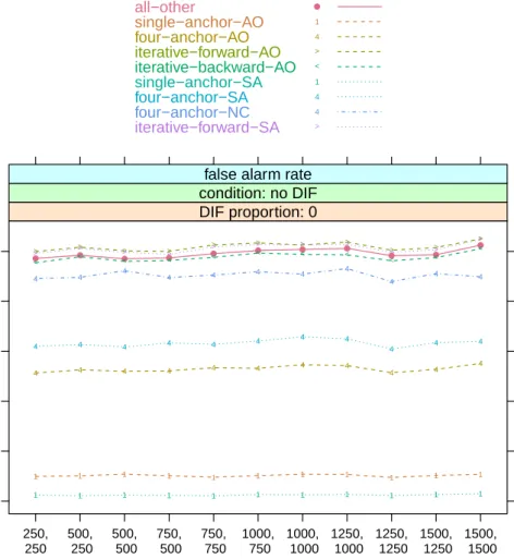
False alarm rates
The estimated false alarm rates are depicted in Figure 2 and (for equal sample sizes to save space) also reported together with their standard errors in Table 2 in the Appendix. As shown in Figure 2, all anchor methods hold the 5% level. While methods from the all-other, the iterative backward backward-AO) and the iterative forward class (iterative-forward-SA, iterative-forward-AO) exhaust the significance limit, methods from the constant anchor class (constant single-anchors: single-anchor-AO and single-anchor-SA; constant four-anchors: four-anchor-AO, four-anchor-SA and four-anchor-NC) remain below that level. The constant single-anchors – that consist of an anchor with the constant length of only one item – display false alarm rates not exceeding 0.01, whereas the constant four-anchors display slightly higher false alarm rates (approximately 0.03 for the constant four-anchor-AO as well as for the four-anchor-SA method and about 0.045 for the constant four-anchor-NC method). Hence, DIF tests with an anchor method from the constant anchor class – especially the constant single-anchor methods – are over-conservative.
Summary
All anchor methods hold the significance level. Over-conservative test results are found for the constant anchor methods, whereas the newly suggested forward-AO and iterative-forward-SA methods together with the all-other and the iterative-backward-AO methods ex-haust the significance level.
sample size (reference, focal) false alar m r ate 0.00 0.01 0.02 0.03 0.04 0.05 250, 250 500, 250 500, 500 750, 500 750, 750 1000, 750 1000, 1000 1250, 1000 1250, 1250 1500, 1250 1500, 1500 ● ● ● ● ● ● ● ● ● ● ● 1 1 1 1 1 1 1 1 1 1 1 4 4 4 4 4 4 4 4 4 4 4 > > > > > > > > > > > < < < < < < < < < < < 1 1 1 1 1 1 1 1 1 1 1 4 4 4 4 4 4 4 4 4 4 4 4 4 4 4 4 4 4 4 4 4 4 > > > > > > > > > > > DIF proportion: 0 condition: no DIF false alarm rate
all−other single−anchor−AO four−anchor−AO iterative−forward−AO iterative−backward−AO single−anchor−SA four−anchor−SA four−anchor−NC iterative−forward−SA ● 1 4 > < 1 4 4 >
Figure 2: False alarm rates under the null hypothesis of no DIF.
4.2. Balanced DIF: No advantage for one group
In the balanced condition, a certain proportion of DIF items (15%, 30% or 45%) is present. Each DIF item favors either the reference or the focal group, but the single advantages cancel out.
False alarm rates
Figure 3 (top row) contains the false alarm rates for the balanced condition, reported also for equal sample sizes together with the standard errors in Table 3 in the Appendix. Most methods display well-controlled false alarm rates – similar to the null condition – with the following exceptions: The constant four-anchor-SA and the constant four-anchor-NC method show a false alarm rate that first increases but then decreases again with growing sample size. The same inverse u-shaped pattern occurs in case of unbalanced DIF and will be explained in more detail in Section 6.
Both constant single-anchor methods (single-anchor-AO and -SA) as well as the four-anchor-AO method, again, remain below the significance level. Hence, DIF tests based on the single-anchor-AO, the single-anchor-SA and the four-anchor-AO method are over-conservative.
sample siz e (ref erence , f ocal) hit rate false alar m rate 0.2 0.4 0.6 0.8 1.0 250, 250 500, 250 500, 500 750, 500 750, 750 1000, 750 1000, 1000 1250, 1000 1250, 1250 1500, 1250 1500, 1500 ● ● ● ● ● ● ● ● ● ● ● 1 1 1 1 1 1 1 1 1 1 1 4 4 4 4 4 4 4 4 4 4 4 > > > > > > > > > > > < < < < < < < < < < < 1 1 1 1 1 1 1 1 1 1 1 4 4 4 4 4 4 4 4 4 4 4 4 4 4 4 4 4 4 4 4 4 4 > > > > > > > > > > > DIF propor tion: 0.15
condition: balanced DIF
hit r ate ● ● ● ● ● ● ● ● ● ● ● 1 1 1 1 1 1 1 1 1 1 1 4 4 4 4 4 4 4 4 4 4 4 > > > > > > > > > > > < < < < < < < < < < < 1 1 1 1 1 1 1 1 1 1 1 4 4 4 4 4 4 4 4 4 4 4 4 4 4 4 4 4 4 4 4 4 4 > > > > > > > > > > > DIF propor tion: 0.3
condition: balanced DIF
hit r ate 250, 250 500, 250 500, 500 750, 500 750, 750 1000, 750 1000, 1000 1250, 1000 1250, 1250 1500, 1250 1500, 1500 ● ● ● ● ● ● ● ● ● ● ● 1 1 1 1 1 1 1 1 1 1 1 4 4 4 4 4 4 4 4 4 4 4 > > > > > > > > > > > < < < < < < < < < < < 1 1 1 1 1 1 1 1 1 1 1 4 4 4 4 4 4 4 4 4 4 4 4 4 4 4 4 4 4 4 4 4 4 > > > > > > > > > > > DIF propor tion: 0.45
condition: balanced DIF
hit r ate ● ● ● ● ● ● ● ● ● ● ● 1 1 1 1 1 1 1 1 1 1 1 4 4 4 4 4 4 4 4 4 4 4 > > > > > > > > > > > < < < < < < < < < < < 1 1 1 1 1 1 1 1 1 1 1 4 4 4 4 4 4 4 4 4 4 4 4 4 4 4 4 4 4 4 4 4 4 > > > > > > > > > > > DIF propor tion: 0.15
condition: balanced DIF
false alar m r ate 250, 250 500, 250 500, 500 750, 500 750, 750 1000, 750 1000, 1000 1250, 1000 1250, 1250 1500, 1250 1500, 1500 ● ● ● ● ● ● ● ● ● ● ● 1 1 1 1 1 1 1 1 1 1 1 4 4 4 4 4 4 4 4 4 4 4 > > > > > > > > > > > < < < < < < < < < < < 1 1 1 1 1 1 1 1 1 1 1 4 4 4 4 4 4 4 4 4 4 4 4 4 4 4 4 4 4 4 4 4 4 > > > > > > > > > > > DIF propor tion: 0.3
condition: balanced DIF
false alar m r ate 0.2 0.4 0.6 0.8 1.0 ● ● ● ● ● ● ● ● ● ● ● 1 1 1 1 1 1 1 1 1 1 1 4 4 4 4 4 4 4 4 4 4 4 > > > > > > > > > > > < < < < < < < < < < < 1 1 1 1 1 1 1 1 1 1 1 4 4 4 4 4 4 4 4 4 4 4 4 4 4 4 4 4 4 4 4 4 4 > > > > > > > > > > > DIF propor tion: 0.45
condition: balanced DIF
false alar m r ate all−other single−anchor−A O four−anchor−A O iter ativ e−f orw ard−A O iter ativ e−backw ard−A O
single−anchor−SA four−anchor−SA four−anchor−NC iter
ativ
e−f
orw
ard−SA
● 1 4 > < 1 4 4 >
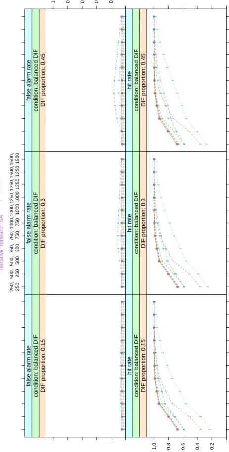
Figure 3: Balanced condition: 15%, 30% and 45% DIF items with no systematic advantage for one group; sample size varies from (250,250) up to (1500,1500); top row: false alarm rates; bottom row: hit rates in the balanced condition.
Hit rates
For DIF test results, hit rates specify how likely true DIF is detected. Figure 3 (bottom row) depicts the hit rates in the balanced condition that increase monotonically with the sample size (for standard errors see also Table 4 in the Appendix). The hit rates that rise slowly correspond to the constant single-anchor methods, but also to the constant four-anchor methods. The methods from the constant anchor class that are combined with the AO-selection (single-anchor-AO, four-anchor-AO) achieve higher hit rates than those combined with the SA-selection (single-anchor-SA, four-anchor-SA) or its modification (four-anchor-NC). In terms of hit rates, all iterative procedures (AO, iterative-forward-SA and iterative-backward-AO) as well as the all-other method show rapidly increasing hit rates that converge to one for sample sizes above 750 in each group.
Summary
In the balanced condition, the AO-selection strategy outperforms the SA-selection by yielding higher hit rates as expected. The difference is large for methods from the constant anchor class, but negligible for methods from the iterative forward anchor class.
All anchor methods show a well-controlled false alarm rate, except the constant four-anchor-SA and the four-anchor-NC method. All iterative methods (from the forward and backward class) and the all-other method display the most rapidly rising hit rates. The newly suggested iterative-forward-AO and iterative-forward-SA method enable a high rate of correctly classi-fied DIF items and simultaneously maintain the significance level in the balanced condition. 4.3. Unbalanced DIF: Advantage for the focal group
In the unbalanced condition, all items simulated with different item parameters favor the focal group. False alarm rates for the unbalanced condition are shown in Figure 4 (top row) and in Table 5 in the Appendix together with the standard errors (again only for settings with equal sample sizes in reference and focal group to save space).
False alarm rates
As opposed to the previous results, in this condition the majority of the anchor methods produce augmented false alarm rates: When the proportion of DIF items increases, the false alarm rates rise as well. Moreover, for most anchor methods, the false alarm rates increase with growing sample size. The settings from the unbalanced condition – especially with 30% and 45% DIF items – are now discussed in more detail in groups of anchor classes.
The all-other method yields the highest false alarm rate in the majority of the simulation settings. The reason for this is that the all-other method is always contaminated in situations where more than one item has DIF. On average, the mean item parameters of the focal group are lower than the mean item parameters of the reference group. These mean differences in the item parameters shift the scales of focal and reference group apart when the all-other method defines the restriction (similar to the instructive example in Section 2). These artificial differences become significant when the sample size increases and, thus, result in an augmented false alarm rate.
For methods from the constant anchor class, the selection strategy explains the false alarm rates: The strategy of selecting anchors based on the DIF tests with all-other items as anchor yields biased DIF test results that induce a high false alarm rate when the sample size is large (as illustrated and discussed in more detail regarding the impact of contamination in
sample siz e (ref erence , f ocal) hit rate false alar m rate 0.2 0.4 0.6 0.8 1.0 250, 250 500, 250 500, 500 750, 500 750, 750 1000, 750 1000, 1000 1250, 1000 1250, 1250 1500, 1250 1500, 1500 ● ● ● ● ● ● ● ● ● ● ● 1 1 1 1 1 1 1 1 1 1 1 4 4 4 4 4 4 4 4 4 4 4 > > > > > > > > > > > < < < < < < < < < < < 1 1 1 1 1 1 1 1 1 1 1 4 4 4 4 4 4 4 4 4 4 4 4 4 4 4 4 4 4 4 4 4 4 > > > > > > > > > > > DIF propor tion: 0.15
condition: unbalanced DIF
hit r ate ● ● ● ● ● ● ● ● ● ● ● 1 1 1 1 1 1 1 1 1 1 1 4 4 4 4 4 4 4 4 4 4 4 > > > > > > > > > > > < < < < < < < < < < < 1 1 1 1 1 1 1 1 1 1 1 4 4 4 4 4 4 4 4 4 4 4 4 4 4 4 4 4 4 4 4 4 4 > > > > > > > > > > > DIF propor tion: 0.3
condition: unbalanced DIF
hit r ate 250, 250 500, 250 500, 500 750, 500 750, 750 1000, 750 1000, 1000 1250, 1000 1250, 1250 1500, 1250 1500, 1500 ● ● ● ● ● ● ● ● ● ● ● 1 1 1 1 1 1 1 1 1 1 1 4 4 4 4 4 4 4 4 4 4 4 > > > > > > > > > > > < < < < < < < < < < < 1 1 1 1 1 1 1 1 1 1 1 4 4 4 4 4 4 4 4 4 4 4 4 4 4 4 4 4 4 4 4 4 4 > > > > > > > > > > > DIF propor tion: 0.45
condition: unbalanced DIF
hit r ate ● ● ● ● ● ● ● ● ● ● ● 1 1 1 1 1 1 1 1 1 1 1 4 4 4 4 4 4 4 4 4 4 4 > > > > > > > > > > > < < < < < < < < < < < 1 1 1 1 1 1 1 1 1 1 1 4 4 4 4 4 4 4 4 4 4 4 4 4 4 4 4 4 4 4 4 4 4 > > > > > > > > > > > DIF propor tion: 0.15
condition: unbalanced DIF
false alar m r ate 250, 250 500, 250 500, 500 750, 500 750, 750 1000, 750 1000, 1000 1250, 1000 1250, 1250 1500, 1250 1500, 1500 ● ● ● ● ● ● ● ● ● ● ● 1 1 1 1 1 1 1 1 1 1 1 4 4 4 4 4 4 4 4 4 4 4 > > > > > > > > > > > < < < < < < < < < < < 1 1 1 1 1 1 1 1 1 1 1 4 4 4 4 4 4 4 4 4 4 4 4 4 4 4 4 4 4 4 4 4 4 > > > > > > > > > > > DIF propor tion: 0.3
condition: unbalanced DIF
false alar m r ate 0.2 0.4 0.6 0.8 1.0 ● ● ● ● ● ● ● ● ● ● ● 1 1 1 1 1 1 1 1 1 1 1 4 4 4 4 4 4 4 4 4 4 4 > > > > > > > > > > > < < < < < < < < < < < 1 1 1 1 1 1 1 1 1 1 1 4 4 4 4 4 4 4 4 4 4 4 4 4 4 4 4 4 4 4 4 4 4 > > > > > > > > > > > DIF propor tion: 0.45
condition: unbalanced DIF
false alar m r ate all−other single−anchor−A O four−anchor−A O iter ativ e−f orw ard−A O iter ativ e−backw ard−A O
single−anchor−SA four−anchor−SA four−anchor−NC iter
ativ
e−f
orw
ard−SA
● 1 4 > < 1 4 4 >
Figure 4: Unbalanced condition: 15%, 30% and 45% DIF items favoring the focal group; sample size varies from (250,250) up to (1500,1500); top row: false alarm rates; bottom row: hit rates in the unbalanced condition.
Section 5).
Constant anchors selected by the single-anchor strategy produce lower false alarm rates in regions of medium or large sample sizes. Here, again, an inversely u-shaped form is visible. After a certain point, the false alarm rates decrease again (a detailed explanation will be given in Section 6). The constant single-anchor methods show lower false alarm rates than the corresponding constant four-anchor methods. For all constant methods, the single-anchor-SA method has the lowest false alarm rate when the sample size is large. Only in the condition with 45% DIF items, it systematically exceeds the significance level at medium sample sizes. The method from the iterative backward anchor class, which starts the initial step by using the all-other method, also leads to augmented false alarm rates (with a maximum observed rate of 0.31 for the highest sample size in case of 45% DIF) that rise when sample size increases. Methods from the iterative forward class display heterogeneous false alarm rates. The iterative-forward-AO method leads to increased false alarm rates – similar to the constant methods with the AO-selection criterion – in the setting with 30% or 45% DIF (up to 0.57 for the highest sample size). The clearly best iterative method in terms of a low false alarm rate is the new iterative-forward-SA method (yielding a false alarm rate of 0.06 for the highest sample size in case of 45% DIF and an observed maximum of 0.24).
Hit rates
The hit rate in the unbalanced condition (cf. Figure 4 (bottom row) and Table 6 in the Appendix) in the settings of larger proportions of DIF items is different: Generally, the over-all level of the hit rate is lower. The rise of the hit rates with the sample size is slow for the methods from the constant anchor class as well as for the all-other method. These methods also have lower hit rates compared to the methods from the iterative forward or backward class that are the only methods that display rapidly increasing and high hit rates. The new iterative forward-SA method provides the highest hit rate and a rapid rise of the hit rate with increasing sample size.
The SA-selection strategy in combination with methods from the constant anchor class is more suitable than the AO-selection strategy regarding the hit rates when the sample size is large. The four-anchor-SA method outperforms the modified constant four-anchor method (four-anchor-NC) in terms of higher hit rates (and lower false alarm rates). The iterative forward procedure with the SA-selection is equal or superior to the iterative-forward-AO method over the entire range of simulated sample sizes.
Summary
In the unbalanced condition, the SA-selection strategy is superior to the AO-selection strategy when the sample size and the DIF proportion are high as expected, since it not only allows a higher hit rate but it also corresponds to a lower false alarm rate.
In the condition of unbalanced DIF, the false alarm rates are no longer well-controlled. When the DIF proportion is high, only the single-anchor-SA and the iterative-forward-SA method have low false alarm rates in regions of large sample sizes. Both constant single-anchor methods yield low false alarm rates – but also low hit rates – when the sample size is small. All methods from the constant anchor class, especially in regions of small sample sizes, show poor hit rates. The highest hit rate – in all settings from the unbalanced condition – corresponds to the newly proposed iterative-forward-SA method.
5. The impact of anchor contamination
As discussed in Section2the contamination of the anchor may induce artificial DIF and thus induce a seriously inflated false alarm rate. Short anchors are preferred in the constant anchor class in order to minimize the risk of contamination that includes only the information whether all anchor items are DIF-free or not (e.g., Shih and Wang 2009). When new anchor methods are proposed, they are judged by their ability to correctly locate a completely DIF-free anchor in order to avoid anchor contamination (e.g., Wang et al. 2012). Since contamination is an important argument in the construction of new anchor methods and since it affects the results of DIF detection (see Section2), we will take a deeper look at the simulation results focussing on the aspect of anchor contamination.
For one exemplary simulation setting, the extreme condition of unbalanced DIF where 45% of the items favor the focal group will now be discussed in more detail in groups of anchor classes to illustrate the impact of contamination.
Figure5(top row) depicts the proportion of replications where at least one item of the anchor is a DIF item (top-left) – this is referred to as risk of contamination – and the proportion of DIF items in the anchor when the anchor is contaminated (top-right) – this is referred to as
degree of contamination. The false alarm rates including only the replications that resulted
in a contaminated anchor are displayed in Figure 5 (bottom-left) next to the false alarm rates including only the replications that resulted in a pure anchor (bottom-right). If no pure replications resulted, the respective false alarm rate is omitted.
The results show the following: For the all-other method all items function as anchor items. Due to the fact that more than one item has DIF in our simulation design, the anchor is contaminated in 100% of the replications. The proportion of DIF items in the anchor is 45% as simulated. With increasing sample size, the power of detecting artificial DIF (DIF-free items that display DIF due to the anchor method chosen) increases and, thus, the false alarm rate rises.
Methods from the constant anchor class are investigated next. The risk of contaminated anchors decreases when the sample size increases. The anchor selection strategy determines how rapidly: When the SA-selection strategy chooses the anchor, the convergence to zero percent contamination is clearly visible in the simulated range of the sample size. The AO-selection strategy shows a decreasing tendency, but even when 1500 observations for each group are available, 70% of the anchors are still contaminated for the four-anchor-AO and 17% for the single-anchor-AO method.
If the constant single-anchors are contaminated, this means that the single anchor item has DIF and, inevitably, the false alarm rates explode when the sample size is large enough to detect significant artificial DIF (in case of 1500 observations in each group: single-anchor-AO: 0.70, single-anchor-SA: 0.54).
Surprisingly, there is a large gap between the degree of contamination for the constant four-anchor methods: When the AO-strategy or the SA-strategy are directly chosen and the sample size is large, on average about one out of four anchor items has DIF. In contrast to this, about three out of four anchor items have DIF when the four-anchor-NC method is chosen. In contaminated situations, consequently, the four-anchor-NC method corresponds to a larger false alarm rate (observed maximum: 0.75) than the four-anchor-AO (observed maximum: 0.54) or the four-anchor-SA method (observed maximum: 0.36). Therefore, the NC method corresponds to larger false alarm rates compared to the four-anchor-SA method over all unbalanced conditions with 45% DIF items (see again Figure4, top row), even though it has a lower risk of contamination. Hence, the degree of contamination is
sample size (reference, focal) 0.0 0.2 0.4 0.6 0.8 1.0 250, 250 500, 250 500, 500 750, 500 750, 750 1000, 750 1000, 1000 1250, 1000 1250, 1250 1500, 1250 1500, 1500 ● ● ● ● ● ● ● ● ● ● ● 1 1 1 1 1 1 1 1 1 1 1 4 4 4 4 4 4 4 4 4 4 4 > > > > > > > > > > > < < < < < < < < < < < 1 1 1 1 1 1 1 1 1 1 1 4 4 4 4 4 4 4 4 4 4 4 4 4 4 4 4 4 4 4 4 4 4 > > > > > > > > > > > DIF proportion: 0.45
condition: unbalanced DIF false alarm rate (contaminated anchor)
1 1 1 1 1 1 1 1 1 1 1 4 4 4 4 4 4 4 4 4 4 4 < < < < < < < < < 1 1 1 1 1 1 1 1 1 1 1 4 4 4 4 4 4 4 4 4 4 4 4 4 4 4 4 4 4 4 4 4 4 > > > > > > > > DIF proportion: 0.45
condition: unbalanced DIF false alarm rate (pure anchor)
● ● ● ● ● ● ● ● ● ● ● 1 1 1 1 1 1 1 1 1 1 1 4 4 4 4 4 4 4 4 4 4 4 > > > > > > > > > > > < < < < < < < < < < < 1 1 1 1 1 1 1 1 1 1 1 4 4 4 4 4 4 4 4 4 4 4 4 4 4 4 4 4 4 4 4 4 4 > > > > > > > > > > > DIF proportion: 0.45
condition: unbalanced DIF risk of contamination 250, 250 500, 250 500, 500 750, 500 750, 750 1000, 750 1000, 1000 1250, 1000 1250, 1250 1500, 1250 1500, 1500 0.0 0.2 0.4 0.6 0.8 1.0 ● ● ● ● ● ● ● ● ● ● ● 1 1 1 1 1 1 1 1 1 1 1 4 4 4 4 4 4 4 4 4 4 4 > > > > > > > > > > > < < < < < < < < < < < 1 1 1 1 1 1 1 1 1 1 1 4 4 4 4 4 4 4 4 4 4 4 4 4 4 4 4 4 4 4 4 4 4 > > > > > > > > > > > DIF proportion: 0.45
condition: unbalanced DIF degree of contamination all−other single−anchor−AO four−anchor−AO iterative−forward−AO iterative−backward−AO single−anchor−SA four−anchor−SA four−anchor−NC iterative−forward−SA ● 1 4 > < 1 4 4 >
Figure 5: Condition of unbalanced DIF with 45% DIF items favoring the focal group; sample size ranges from (250,250) to (1500,1500); top-left: risk of contaminated anchors (at least one DIF item included in the anchor); top-right: degree of contamination (proportion of DIF items in contaminated anchors); bottom-left: false alarm rates when the anchor is contaminated; bottom-right: false alarm rates when the anchor is pure.
important for the results of the DIF assessment.
If the anchor is pure, the false alarm rates for the constant four-anchor method located by the SA-selection strategy (or the NC-selection) are lower. Note, however, that even if the anchor is pure, the false alarm rates of the constant anchor methods exceed the significance level. To clarify this fact, we will present an additional simulation study in the next section.
The methods from the iterative forward and backward anchor class are more often contami-nated than the constant single-anchors (see Figure5). This is not surprising, as the anchors in-clude more items. Similar to the all-other method, all replications of the iterative-forward-AO method are contaminated. The iterative-forward-SA and the iterative-backward-AO method yield a risk of contamination that decreases with the sample size (minimum 0.26 and 0.40 in the simulated range). In case of contaminated anchors, the methods from the iterative forward and backward class also produce augmented false alarm rates. When the sample size in each group exceeds 750, the iterative-forward-SA method definitely has the lowest false alarm rate. When the sample size is 1000 in each group, the mean false alarm rate of the iterative-forward-SA method including all replications does not even exceed the mean false alarm rate of all three constant four-anchor methods including only the pure replications while simultaneously the hit rate is higher for the iterative-forward-SA method.
Our findings clarify that it is not the risk of contamination alone that explains the augmented false alarm rates. The best method in the unbalanced condition when the sample size is large is the iterative-forward-SA method even if it has a high risk of contamination. Nevertheless, the iterative-forward-SA method displays a low false alarm rate and also a high hit rate. Therefore, the consequences of contamination depend on the degree of contamination which is low for this method due to the SA-selection strategy that is suitable for unbalanced DIF. Research on DIF analysis and anchor selection procedures should, thus, not only concentrate on the risk of contamination, but also focus on the consequences, which strongly depend on the proportion of contaminated items in the anchor.
6. Characteristics of the anchor items inducing artificial DIF
In our simulation study, several anchor methods – especially the four-anchor-SA and the four-anchor-NC method – display inversely u-shaped false alarm rates that are yet to be explained. There are two mechanisms at work here: On one hand, the risk and the degree of contamination decrease with increasing sample size when the anchor selection strategy works appropriately and, thus, the extent of artificial DIF decreases. On the other hand, the power of detecting artificial DIF increases with growing sample size. One possible explanation for the inversely u-shaped pattern is the interaction between the decreasing extent of artificial DIF induced by anchor contamination and the increasing power of detecting statistically significant artificial DIF. In the beginning the false alarm rate increases due to the increasing power for detecting artificial DIF but at some point the false alarm rate decreases again as the risk of contamination decreases. This explanation is consistent with the findings from Section 5, where the anchor is contaminated: The four-anchor-SA method, for example, displays a degree of contamination that decreases with sample size (see again Figure 5, top-right) and an inversely u-shaped false alarm rate when the anchor is contaminated (see again Figure 5, bottom-left).However, with this argument we cannot yet explain why the false alarm rates show the same pattern for pure (uncontaminated) replications (see again Figure 5, bottom-right). Here, the single-anchor-SA, the four-anchor-SA as well as the four-anchor-NC method display inversely