Practical Recommendations on Crawling
Online Social Networks
Minas Gjoka, Maciej Kurant, Carter T. Butts, and Athina Markopoulou,
IEEE Member
Abstract—Our goal in this paper is to develop a practical framework for obtaining a uniform sample of users in an online social network (OSN) by crawling its social graph. Such a sample allows to estimate any user property and some topological properties as well. To this end, first, we consider and compare several candidate crawling techniques. Two approaches that can produce approximately uniform samples are the Metropolis-Hasting random walk (MHRW) and a re-weighted random walk (RWRW). Both have pros and cons, which we demonstrate through a comparison to each other as well as to the “ground truth.” In contrast, using Breadth-First-Search (BFS) or an unad-justed Random Walk (RW) leads to substantially biased results. Second, and in addition to offline performance assessment, we introduce online formal convergence diagnostics to assess sample quality during the data collection process. We show how these diagnostics can be used to effectively determine when a random walk sample is of adequate size and quality. Third, as a case study, we apply the above methods toFacebookand we collect the first, to the best of our knowledge, representative sample of
Facebook users. We make it publicly available and employ it to characterize several key properties of Facebook.
Index Terms—Sampling methods, Social network services, Facebook, Random Walks, Convergence, Measurements, Graph sampling.
I. INTRODUCTION
Online Social Networks (OSNs) have recently emerged as a new Internet “killer-application.” The adoption of OSNs by Internet users is off-the-charts with respect to almost every metric. In November 2010, Facebook, the most popular OSN, counted more than 500 million members; the total combined membership in the top five OSNs (Facebook,
QQ,Myspace,Orkut,Twitter) exceeded 1 billion users. Putting this number into context, the population of OSN users is approaching 20% of the world population and is more than 50% of the world’s Internet users. According to Nielsen [1], users worldwide currently spend over 110 billion minutes on social media sites per month, which accounts for 22% of all time spent online, surpassing even time spent on email. According to Alexa [2], a well-known traffic analytics website,
Facebookis the second most visited website on the Internet All authors are affiliated with the California Institute for Telecommuni-cations and Information Technology (CalIT2) at the University of California, Irvine, CA 92697-2800. Carter T. Butts is also with the Sociology Department at UC Irvine. Athina Markopoulou is with the EECS Department at UC Irvine and with the Center for Pervasive Communications and Computing (CPCC). Email:{mgjoka, mkurant, buttsc, athina}@uci.edu.
This work has been supported by the following grants: NSF CDI award 1028394, AFOSR FA9550-10-1-0310, AFOSR Award FA9550- 09-0643; SNF grant PBELP2-130871, Switzerland; and DOD ONR award N00014-08-1-1015.
Manuscript received on December 15 2010; revised on June 1st 2011.
(second only to Google) with each user spending 30 minutes on average per day on the site (more than the time spent on Google). Four of the top five OSNs are also contained in Alexa’s top 15 websites in regard to traffic rankings. Clearly, OSNs in general, and Facebookin particular, have become an important phenomenon on the Internet.
OSNs are of interest to several different communities. For example, sociologists employ them as a venue for collecting relational data and studying online human behavior. Marketers, by contrast, seek to exploit information about OSNs in the design of viral marketing strategies. From an engineering perspective, understanding OSNs can enable the design of better networked systems. For example, an OSN provider may want to understand the social graph and user activity in order to improve user experience by optimizing the design of their datacenters and/or data storage on the cloud [3]; or by providing personalized services and ads. A network provider may also want to understand the traffic generated by activities of OSN users in order to design mechanisms, such as caching [4] and traffic engineering [5], to better serve that traffic.
Another potential use of OSNs is in algorithms that employ trusted or influential users,e.g., to thwart unwanted commu-nication while not impeding legitimate commucommu-nication [6]; to utilize social trust for collaborative spam filtering [7]; or to en-able online personas to cost-effectively obtain credentials [8]. Third-party applications are also interested in OSNs in order to provide personalized services as well as to become popular. The immense interest generated by OSNs has given rise to a number of measurement and characterization studies that attempt to provide a first step towards their understanding. Only a very small number of these studies are based on complete datasets provided by the OSN operators [9,10]. A few other studies have collected a complete view of specific parts of OSNs; e.g., [11] collected the social graph of the Harvard university network. However, the complete dataset is typically unavailable to researchers, as most OSNs are unwilling to share their company’s data even in an anonymized form, primarily due to privacy concerns.
Furthermore, the large size1 and access limitations of most
OSN services (e.g., login requirements, limited view, API query limits) make it difficult or nearly impossible to fully 1 A back-of-the-envelope calculation of the effort needed to crawl
Facebook’s social graph is as follows. In December 2010, Facebook advertised more than 500 million active users, each encoded by 64 bits (4 bytes) long userID, and 130 friends per user on average. Therefore, the raw topological data alone, without any node attributes, amounts to at least 500M×130×8bytes≃520GBytes.
cover the social graph of an OSN. In many cases, HTML scraping is necessary, which increases the overhead multifold.2
Instead, it would be desirable to obtain and use a small but representative sample.
Given this, sampling techniques are essential for practical estimation of OSN properties. While sampling can, in princi-ple, allow precise population-level inference from a relatively small number of observations, this depends critically on the ability to draw a sample with known statistical properties. The lack of a sampling frame (i.e.,a complete list of users, from which individuals can be directly sampled) for most OSNs makes principled sampling especially difficult. To elude this limitation, our work focuses on sampling methods that are based on crawling of friendship relations - a fundamental primitive in any OSN.
Our goal in this paper is to provide a framework for obtaining an asymptotically uniform sample (or one that can be systematically reweighted to approach uniformity) of OSN users by crawling the social graph. We provide practical recommendations for appropriately implementing the frame-work, including: the choice of crawling technique; the use of online convergence diagnostics; and the implementation of high-performance crawlers. We then apply our framework to an important case-study - Facebook. More specifically, we make the following three contributions.
Our first contribution is the comparison of several candidate graph-crawling techniques in terms of sampling bias and efficiency. First, we consider BreadthFirstSearch (BFS) -the most widely used technique for measuring OSNs [9,12] including Facebook [13]. BFS sampling is known to in-troduce bias towards high degree nodes, which is highly non-trivial to characterize analytically [14,15] or to correct. Second, we consider Random Walk (RW) sampling, which also leads to bias towards high degree nodes, but whose bias can be quantified by Markov Chain analysis and corrected via appropriate re-weighting (RWRW) [16,17]. Then, we consider the Metropolis-Hastings Random Walk (MHRW) that can directly yield a uniform stationary distribution of users. This technique has been used in the past for P2P sampling [18], recently for a few OSNs [19,20], but not for Facebook. Finally, we also collect a uniform sample of Facebook
userIDs (UNI), selected by a rejection sampling procedure from Facebook’s 32-bit ID space, which serves as our “ground truth”. We compare all sampling methods in terms of their bias and convergence speed. We show that MHRW and RWRW are both able to collect asymptotically uniform samples, while BFS and RW result in a significant bias in practice. We also compare the efficiency MHRW to RWRW, via analysis, simulation and experimentation and discuss their pros and cons. The former provides a sample ready to be used by non-experts, while the latter is more efficient for all practical purposes.
Our second contribution is that we introduce, for the first time in this context, the use of formal convergence diagnostics (namely Geweke and Gelman-Rubin) to assess sample quality 2For the example in footnote 1, one would have to download about500M× 230KBytes≃115T Bytesof uncompressed HTML data.
in an online fashion. These methods (adapted from Markov Chain Monte Carlo applications) allow us to determine, in the absence of a ground truth, when a sample is adequate for use, and hence when it is safe to stop sampling. These is a critical issue in implementation.
Our third contribution is that we apply and compare all the aforementioned techniques for the first time, to the best of our knowledge, on a large scale OSN. We use Facebook
as a case study by crawling its web front-end, which is highly non-trivial due to various access limitations, and we provide guidelines for the practical implementation of high-performance crawlers. We obtain the first representative sam-ple of Facebook users, which we make publicly avail-able [21]; we have received approximately 500 requests for this dataset in the last eighteen months. Finally, we use the collected datasets to characterize several key properties of
Facebook, including user properties (e.g., privacy settings) and topological properties (e.g., the node degree distribution, clustering, and assortativity).
The structure of this paper is as follows. Section II discusses related work. Section III describes the sampling methodol-ogy, including the assumptions and limitations, the candi-date crawling techniques and the convergence diagnostics. Section IV describes the data collection process, including the implementation of high-performance crawlers, and the collected data sets from Facebook. Section V evaluates and compares all sampling techniques in terms of efficiency (convergence of various node properties) and quality (bias) of the obtained sample. Section VI provides a characterization of some key Facebook properties, based on the MHRW sample. Section VII concludes the paper. The appendices elaborate on the following points: (A) the uniform sample obtained via userID rejection sampling, used as “ground truth” in this paper; (B) the lack of temporal dynamics inFacebook, in the timescale of our crawls; and (C) a comparison of the sampling efficiency of MHRW vs. RWRW.
II. RELATEDWORK
Broadly speaking, there are two bodies of work related to this paper: (i) sampling techniques, investigating the quality and efficiency of the sampling technique itself and (ii) charac-terization studies, focusing on the properties of online social networks based on the collected data. In this section, we review this related literature and place our work in perspective.
A. Graph sampling techniques
Graph sampling techniques, via crawling, can be roughly classified into two categories: graph traversal techniques and random walks. Ingraph traversal techniques, nodes are sam-pled without replacement: once a node is visited, it is not visited again. These methods differ in the order in which they visit the nodes; examples include Breadth-Search-First (BFS), Depth-First Search (DFS), Forest Fire (FF) and Snowball Sampling (SBS) [22].
BFS, in particular, is a basic technique that has been used extensively for sampling OSNs in past research [9,12, 13,23,24]. One reason for this popularity is that an (even
incomplete) BFS sample collects a full view (all nodes and edges) of some particular region in the graph. However, BFS has been shown to lead to a bias towards high degree nodes in various artificial and real world topologies [25]–[27]. Our work also confirms the bias of BFS when sampling Online Social Networks. It is worth noting that BFS and its variants lead to samples that not only are biased but also do not have known statistical properties (and hence cannot in general be used to produce trustworthy estimates). Although recent work suggests that it is possible to analytically compute and correct this bias for random graphs with certain degree distributions [14], these methods are mere heuristics under arbitrary graphs [15] and will fail for networks with large-scale heterogeneity (e.g.,block structure).
Random walks on graphsare a well-studied topic; see [28] for an excellent survey. They have been used for sampling the World Wide Web (WWW) [29,30], peer-to-peer networks [17, 18,31], and other large graphs [32]. Similarly to traversals, random walks are typically biased towards high-degree nodes. However, the bias of random walks can be analyzed and corrected for using classical results from Markov Chains. If necessary, such a bias correction can be obtained during the walk itself - the resulting Metropolis-Hasting Random Walk (MHRW) described in Section III-C4 has been applied by Stutzbach et al. [18] to select a representative sample of peers in the Gnutella network. Alternatively, we can re-weight the sample after it is collected - the resulting Re-Weighted Random Walk (RWRW) described in Section III-C3 has been recently compared with MHRW in the context of peer-to-peer sampling by Rastiet al.[17]. Further improvements or variants of random walks include random walk with jumps [29,33], multiple dependent random walks [34], weighted random walks [35], or multigraph sampling [36].
Our work is most closely related to the random walk techniques. We obtain unbiased estimators of user properties inFacebookusing MHRW and RWRW and we compare the two through experiments and analysis; BFS and RW (without re-weighting) are used mainly as baselines for comparison. We complement the crawling techniques with formal, online convergence diagnostic tests using several node properties.To the best of our knowledge, this has not been done before in measurements of such systems. The closest to formal diagnostics is the work by Latapy et al. [37] which studies how the properties of interest evolve when the sample grows to practically detect steady state. We also implementmultiple parallel chains. Multiple chains started at the same node have been recently used in [17]. In contrast, we start different chains from different nodes. We demonstrate that random walks, whose bias can be analyzed and corrected, are able to estimate properties of users in OSNs remarkably well in practice. We also find that correcting for the bias at the end (RWRW), rather than during the walk (MHRW) is more efficient for all practical purposes - a finding that agrees with [17].
In terms of application, we apply the measurement tech-niques to online social networks and study characteristics specific to that context. To the best of our knowledge, we are the first to obtain an unbiased sample of a large scale OSN, namely Facebook, and make it publicly available.
Krishnamurthy et al. [20] ran a single Metropolis Random Walk, inspired by [18], on Twitter as a way to verify the lack of bias in their main crawl used throughout the paper. However, the Metropolis algorithm was not the main focus of their paper and Twitter is a directed graph which requires different treatment. Parallel to our work, Rastiet al.[19] also applied similar random walk techniques to collect unbiased samples of Friendster.
Previous work on thetemporal dynamicsof social networks includes [19,38]–[41]. Kumaret al.[38] studied the structure and evolution of Flickr and Yahoo! from datasets provided by the OSN providers. Backstromet al.[39] presented different ways in which communities in social networks grow over time and [40] proposed a method for modeling relationships that change over time in a social network. Willingeret al.[41] pro-posed a multi-scale approach to study dynamic social graphs at a coarser level of granularity. Rasti et al. [19] evaluate the performance of random walks in dynamic graphs via simulations and show that there is a tradeoff between number of parallel samplers, churn and accuracy. In our work, we assume that the social graph remains static during the crawl, which we show in Appendix B to be the case forFacebook
in practice. Therefore, we do not consider dynamics, which are essential in other sampling contexts.
A unique asset of our study is the collection of a true uniform sample of OSN users through rejection sampling of userIDs (UNI), which served as ground truth in this paper; see Section III-D. We note that UNI yields a uniform sample of users regardless of the allocation policy of userIDs by the OSN, as shown in Appendix A. UNI is essentially a star random node sampling scheme [42]; this is different from the induced subgraph random node sampling schemes that were evaluated in [32,43].
B. Characterization studies of OSNs
Several papers have measured and characterized properties of OSNs. In [44], Krishnamurthy presents a summary of the challenges that researchers face in collecting data from OSNs. In [9], Ahnet al.analyze three online social networks; one complete social graph of Cyworld obtained from the
Cyworld provider, and two small samples from Orkut
and Myspacecrawled with BFS. In [12,23], Mislove et al.
studied the properties of the social graph in four popular OSNs: Flickr, LiveJournal, Orkut, and YouTube. Their approach was to collect the large Weakly Connected Component, also using BFS; their study shows that OSNs are structurally different from other complex networks.
[11,13,45] are related to this paper in that they also study
Facebook. Wilson et al. [13] collect and analyze social graphs and user interaction graphs in Facebook between March and May 2008. Their methodology is what we refer to as Region-Constrained BFS: they exhaustively collect all open user profiles and their list of friends in the largest regional networks. Such Region-Constrained BFS might be appropriate to study particular regions, but it does not provideFacebook -wide information, which is the goal of this paper. Furthermore, the percentage of users in the social graph retrieved in [13] is
30%-60% less than the maximum possible in each network.3
Our findings show some noteworthy differences from [13]: for example, we find larger values of the degree-dependent clus-tering coefficient, significantly higher assortativity coefficient, and a degree distribution that does not follow a power law. Finally, Wilsonet al.[13] focus on the user interaction graph, while we focus on the friendship graph. [11] and [45] have also made publicly available and analyzed datasets corresponding to university networks fromFacebookwith many annotated properties for each student. In contrast, we collect a sample of the globalFacebooksocial graph.
Other works that have measured properties of Facebook
include [24,46]–[48]. In [46], Krishnamurthy et al. examine the usage of privacy settings in Myspace and Facebook, and the potential privacy leakage in OSNs. Compared to that work, we have one common privacy attribute, “View friends“, for which we observe similar results using our unbiased sample. We also have additional privacy settings and the one-hop neighborhood for every node, which allows us to analyze user properties conditioned on their privacy awareness. Bonneau et al. [47] demonstrate that many interesting user properties can be accurately approximated just by crawling “public search listings”.
Finally, there is a large body of work on the collection and analysis of datasets for platforms or services that are not pure online social networks but include social networking features. To mention a few examples, Liben-Nowellet al.[49] studied the LiveJournalonline community and showed a strong relationship between friendship and geography in social networks. Cha et al. [50] presented a data-driven analysis of user generated content video popularity distributions by using data collected fromYouTubeandDaum. Gillet al.[51] also studied a wide range of features of YouTubetraffic, includ-ing usage patterns, file properties, popularity and referencinclud-ing characteristics. In [36], we crawlLast.FMa music site with social networking features.
C. Our prior and related work.
The conference version of this work appeared in [52]. This paper is revised and extended to include the following materials. (i) A detailed discussion of the uniform userID rejection sampling, which is used as ground truth in this work; see Section III-D and Appendix A. (ii) An empirical validation of the assumption that the social graph is static in the time scales of the crawl; see Appendix B. (iii) A detailed comparison of MHRW and RWRW methods and the finding that RWRW is more efficient for all practical purposes; see Section V-A for an experimental comparison on Facebook
and Appendix C for a comparison via analysis and simulation. (iv) An extended section on the characterization ofFacebook
based on a representative sample; see Section VI for additional figures on node properties and topological characteristics, and 3More specifically, it is most likely that for the collection of the social graph, their BFS crawler does not follow users that have their “view profile” privacy setting closed and “view friends“ privacy setting open.We infer that, by the discrepancy in the percentage of users for those settings as reported in aFacebookprivacy study conducted during the same time in [46] i.e.,in networks New York, London, Australia, Turkey.
new results on privacy settings. (iv) A comprehensive review of related work in this section.
This work focuses on providing a practical sampling frame-work (e.g., choosing a crawling method, utilizing online convergence diagnostics, implementation issues) for a well-connected OSN social graph. Other related -but distinct-work from our group that appear in the same issue include: (i) multigraph sampling[36], a method that utilizes multiple relations to crawl the social graph and is well suited for OSNs with either poorly connected or highly clustered users, (ii) a BFS bias correction procedure [15].
III. SAMPLINGMETHODOLOGY
We consider OSNs, whose social graph can be modeled as a graphG= (V, E), whereV is a set of nodes (users) andE
is a set of edges.
A. Assumptions
We make the following assumptions and discuss the extent to which they hold:
A1 Gis undirected.This is true inFacebook(its friendship relations are mutual), but in Twitter the edges are directed, which significantly changes the problem [20,29,53]. A2 We are interested only in the publicly available part ofG.
This is not a big limitation inFacebook, because all the information we collect is publicly available under default privacy settings.
A3 Gis well connected, and/or we can ignore isolated nodes.
This holds relatively well in Facebook thanks to its high connection density. In contrast, in Last.fm the friendship graph is highly fragmented, which may require more sophisticated crawling approaches [36].
A4 G remains static during the duration of our crawl. We argue in Appendix B that this assumption holds well in
Facebook.
A5 The OSN supports crawling.This means that on sampling a node v we learn the identities of all its neighbors. It is typically true in OSNs,e.g.,through some mechanism such as an API call or HTML scraping (both available in
Facebook).
B. Goal and applications
Our goal is to obtain a uniform sample (or more generally a probability sample) of OSN users by crawling the social graph. This is interesting in its own right, as it allows to estimate frequencies of user attributes such as age, privacy settings etc. Furthermore, a probability sample of users allows us to estimate some local topological properties such as node degree distribution, clustering and assortativity. In Section VI-A, we compute the last two properties based on the one-hop neighborhood of nodes. Therefore, a random sample of nodes, obtained using our methodology, is a useful building block towards characterizing structural properties.
We would like to emphasize, however, that a sample of nodes cannot be directly used to obtain a “representative topol-ogy” for estimating global structural properties. For example,
the nodes and edges in the sample, possibly together with their neighbors (nodes and edges in the egonets) donotnecessarily provide a graph representative of the entire Facebook with respect to properties such as e.g., geodesics. Therefore, if global structural properties rather than local properties or user attributes are of interest, our node sampling needs to be combined with other techniques such as matrix completion [54] or block modeling [55].
C. Sampling via crawling
The process of crawling the social graph starts with an initially selected node and proceeds iteratively. In every op-eration, we visit a node and discover all its neighbors. There are many ways in which we can proceed, depending on which neighbor we choose to visit next. In this section, we describe the sampling methods implemented and compared in this paper.
1) Breadth First Search (BFS): At each new iteration the earliest explored but not-yet-visited node is selected next. As this method discovers all nodes within some distance from the starting point, an incomplete BFS is likely to densely cover only some specific region of the graph.
2) Random Walk (RW): In the classic random walk [28], the next-hop node w is chosen uniformly at random among the neighbors of the current node v. I.e., the probability of moving fromv tow is PRW v,w = 1 kv ifw is a neighbor ofv, 0 otherwise.
RW is inherently biased. Assuming a connected graph and aperiodicity, the probability of being at the particular nodev
converges to the stationary distribution πRW
v = k
v
2·|E|,i.e. the classic RW samples nodes w.p. πRW
v ∼ kv. This is clearly
biased towards high degree nodes;e.g.,a node with twice the degree will be visited by RW twice more often. In Section V, we show that several other node properties are correlated with the node degree and thus estimated with bias by RW sampling.
3) Re-Weighted Random Walk (RWRW): A natural next step is to crawl the network using RW, but to correct for the degree bias by an appropriate re-weighting of the measured values. This can be done using the Hansen-Hurwitz estimator 4 [56]
as first shown in [16,57] for random walks and also later used in [17]. Consider a stationary random walk that has visited
V = v1, ...vn unique nodes. Each node can belong to one
of m groups with respect to a property of interest A, which might be the degree, network size or any other discrete-valued node property. Let (A1, A2, .., Am) be all possible values of
Aand corresponding groups;∪m
1Ai =V.E.g.,if the property
of interest is the node degree, Ai contains all nodes u that
have degree ku =i. To estimate the probability distribution
ofA, we need to estimate the proportion of nodes with value
Ai, i= 1, ..m: ˆ p(Ai) = P u∈Ai1/ku P u∈V 1/ku (1) 4The simple estimators we use in this paper, e.g., see Eq. (1), are Hansen-Hurwitz estimators, which are well-known to have good properties (consistent and unbiased) under mild conditions; see [55] for proof of consistency.
Estimators for continuous properties can be obtained using related methods,e.g., kernel density estimators.
4) Metropolis-Hastings Random Walk (MHRW): Instead of correcting the bias after the walk, one can appropriately mod-ify the transition probabilities so that the walk converges to the desired uniform distribution. The Metropolis-Hastings al-gorithm [58] is a general Markov Chain Monte Carlo (MCMC) technique [59] for sampling from a probability distribution µ
that is difficult to sample from directly. In our case, we would like to sample nodes from the uniform distributionµv =|V1|.
This can be achieved by the following transition probability:
PMH v,w= min(k1v,k1w) ifw is a neighbor ofv, 1−P y6=vP MH v,y ifw=v, 0 otherwise.
It can be shown that the resulting stationary distribution is πM H
v = |V1|, which is exactly the uniform distribution we are looking for. PMH
v,w implies the following algorithm,
which we refer to simply as MHRW in the rest of the paper:
v←initial node.
whilestopping criterion not metdo
Select nodewuniformly at random from neighbors ofv. Generate uniformly at random a number0≤p≤1.
if p≤kkwv then v←w. else Stay atv end if end while
At every iteration of MHRW, at the current node v we randomly select a neighborwand move there w.p.min(1,kv
kw). We always accept the move towards a node of smaller degree, and reject some of the moves towards higher degree nodes. This eliminates the bias towards high degree nodes.
D. Ground Truth: Uniform Sample of UserIDs (UNI)
Assessing the quality of any graph sampling method on an unknown graph, as it is the case when measuring real systems, is a challenging task. In order to have a “ground truth” to compare against, the performance of such methods is typically tested on artificial graphs.
Fortunately,Facebookwas an exception during the time period we performed our measurements. We capitalized on a unique opportunity to obtain a uniform sample ofFacebook
users by generating uniformly random 32-bit userIDs, and by pollingFacebookabout their existence. If the userID exists (i.e.,belongs to a valid user), we keep it, otherwise we discard it. This simple method is a textbook technique known as
rejection sampling[60] and in general it allows to sample from any distribution of interest, which in our case is the uniform. In particular, it guarantees to select uniformly random userIDs from the allocatedFacebookusers regardless of their actual distribution in the userID space, even when the userIDs are not allocated sequentially or evenly across the userID space. For completeness, we re-derive this property in Appendix VII. We refer to this method as “UNI” and use it as a ground-truth uniform sampler.
Although UNI sampling solves the problem of uniform node sampling in Facebook, crawling remains important. Indeed, the userID space must not be sparsely allocated for UNI to be efficient. During our data collection (April-May 2009) the number of Facebookusers (∼200×106) was comparable
to the size of the userID space (232 ∼ 4.3×10⁹), resulting
in about one user retrieved per 22 attempts on average. If the userID were 64 bit long or consisting of strings of arbitrary length, UNI would had been infeasible.5
In summary, we were fortunate to be able to obtain a uniform independence sample of userIDs, which we then used as a baseline for comparison (our “ground truth”) and showed that our results conform closely to it. However, crawling friendship relations is a fundamental primitive available in all OSNs and, we believe, the right building block for designing sampling techniques in OSNs in the general case.
E. Convergence
1) Using Multiple Parallel Walks: Multiple parallel walks are used in the MCMC literature [59] to improve convergence. Intuitively, if we only have one walk, the walk may get trapped in cluster while exploring the graph, which may lead to erroneous diagnosis of convergence. Having multiple parallel walks reduces the probability of this happening and allows for more accurate convergence diagnostics. An additional advan-tage of multiple parallel walks, from an implementation point of view, is that it is amenable to parallel implementation from different machines or different threads in the same machine.
2) Detecting Convergence with Online Diagnostics: Valid inferences from MCMC are based on the assumption that the samples are derived from the equilibrium distribution, which is true asymptotically. In order to correctly diagnose when convergence to equilibrium occurs, we use standard diagnostic tests developed within the MCMC literature [59]. In particular, we would like to use diagnostic tests to answer at least the following questions:
• How many of the initial samples in each walk do we need to discard to lose dependence from the starting point (or burn-in) ?
• How many samples do we need before we have collected a representative sample?
A standard approach is to run the sampling long enough and to discard a number of initial burn-in samples proactively. From a practical point of view, however, the burn-in comes at a cost. In the case ofFacebook, it is the consumed bandwidth (in the order of gigabytes) and measurement time (days or weeks). It is therefore crucial to assess the convergence of our MCMC sampling, and to decide on appropriate settings of burn-in and total running time.
Given that during a crawl we do not know the target distribution, we can only estimate convergence from the sta-tistical properties of the walks as they are collected. Here 5To mention a few such cases in the same time frame:Orkuthad a 64bit userID and hi5 used a concatenation of userID+Name. Interestingly, within days to weeks after our measurements were completed,Facebookchanged its userID allocation space from 32 bit to 64 bit [61]. Section V-B3 contains more information about userID space usage inFacebookin April 2009.
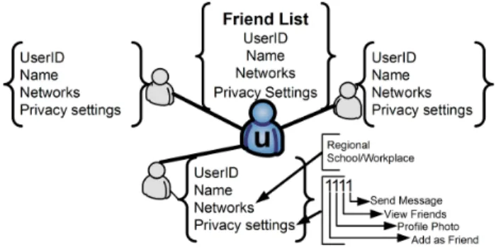
Fig. 1. Basic node information collected when visiting a useru.
we present two standard convergence tests, widely accepted and well documented in the MCMC literature, Geweke [62] and Gelman-Rubin [63], described below. In Section V, we apply these tests on several node properties, including the node degree, userID, network ID and membership in a specific network; please see Section V-A5 for details. Below, we briefly outline the rationale of these tests.
Geweke Diagnostic. The Geweke diagnostic [62] detects
the convergence of a single Markov chain. Let X be a single sequence of samples of our metric of interest. Geweke considers two subsequences ofX, its beginningXa(typically
the first 10%), and its endXb (typically the last 50%). Based
onXa andXb, we compute the z-statistic:
z= p E(Xa)−E(Xb)
V ar(Xa) +V ar(Xb)
With increasing number of iterations,XaandXbmove further
apart, which limits the correlation between them. As they measure the same metric, they should be identically distributed when converged and, according to the law of large numbers, the z values become normally distributed with mean 0 and variance 1. We can declare convergence when all values fall in the[−1,1]interval.
Gelman-Rubin Diagnostic. Monitoring one long sequence
of nodes has some disadvantages. For example, if our chain stays long enough in some non-representative region of the parameter space, we might erroneously declare convergence. For this reason, Gelman and Rubin [63] proposed to monitor
m > 1 sequences. Intuitively speaking, the Gelman-Rubin
diagnostic compares the empirical distributions of individ-ual chains with the empirical distribution of all sequences together: if these two are similar, we declare convergence. The test outputs a single valueR that is a function of means and variances of all chains. With time, R approaches 1, and convergence is declared typically for values smaller than 1.02.
IV. DATACOLLECTION
A. User properties of interest
Fig. 1 summarizes the information collected when visiting the “show friends” web page of a sampled user u, which we refer to asbasic node information.
bit attribute explanation
1 Add as friend =1 ifw can propose to ‘friend’u
2 Photo =1 ifw can see the profile photo ofu
3 View friends =1 ifw can see the friends ofu
4 Send message =1 ifw can send a message tou
TABLE I
PRIVACY SETTINGS OF A USERuWITH RESPECT TO HER NON-FRIENDw.
Name and userID. Each user is uniquely defined by her userID, which is a 32-bit number6. Each user presumably
provides her real name. The names do not have to be unique. Friends list.A core idea in social networks is the possibility to declare friendship between users. InFacebook, friendship is always mutual and must be accepted by both sides. Thus the social network is undirected.
Networks. Facebook uses two types of “networks” to organize its users. The first are regional (geographical) net-works7. There are 507 predefined regional networks that correspond to cities, regions, and countries around the world. A user can freely join any regional network but can be a member of only one regional network at a time. Changes are allowed, but no more than twice every 6 months (April 2009). The second type of networks contain user affiliations with colleges, workplaces, and high schools and have stricter membership criteria: they require a valid email account from the corresponding domain,e.g.,to join the UC Irvine network you have to provide a “@uci.edu” email account. A user can belong to many networks of the second type.
Privacy settings Qv.Each user ucan restrict the amount
of information revealed to any non-friend node w, as well as the possibility of interaction with w. These are captured by four basic binary privacy attributes, as described in Table I. We refer to the resulting 4-bit number as privacy settingsQv
of nodev. By default,FacebooksetsQv= 1111(allow all).
Friends of u. The “show friends” web page of user u
exposes network membership information and privacy settings for each listed friend. Therefore, we collect such information for all friends of u, at no additional cost.
Profiles. Much more information about a user can poten-tially be obtained by viewing her profile. Unless restricted by the user, the profile can be displayed by her friends and users from the same network. In this work, we do not collect any profile information, even if it is publicly available. We study only the basic node information shown in Fig.1.
Ego Networks. The sample of nodes collected by our method enables us to study many features of FB users in a statistically unbiased manner. However, more elaborate topo-logical measures, such as clustering coefficient and assortativ-ity, cannot be easily estimated based purely on a single-node view. For this reason, we decided to also collect a number
6Facebookchanged to 64-bit user ID space after May 2009 [61] whereas our crawls were collected during April-May 2009.
7Regional networks were available at the time of this study but were phased out starting from June 2009 [64]
Fig. 2. (a) Sampled useru with observed edges in yellow color. (b) The extended ego network of useruwith observed nodes and edges in yellow color. Invalid neighborw, whose privacy settingsQw=∗ ∗0∗do not allow friend listing, is discarded.
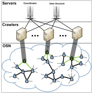
Fig. 3. Distributed Crawling of an Online Social Network
of extended ego nets 8 (see Fig 2), for ∼37K “ego” nodes,
randomly selected from all nodes in MHRW.
B. Crawling Process
In order to apply our methodology to real-life OSNs, we implemented high-performance distributed crawlers that explored the social graph in a systematic and efficient way.
1) Challenges: There are several practical challenges we faced while crawling the social graph of OSNs. First, OSNs usually use some defense mechanisms against automated data mining. Mislove et al. [12] reported rate limits per IP while crawlingOrkut. Similarly, in our Facebook crawls we experienced banned accounts, probably due to excessive traffic. Second, inFacebook, the API calls are usually more restrictive than HTML scraping, which forced us to implement the latter. Third, many modern web sites enable asynchronous 8We use the extended egonet sample differently from the Random Node Neighbor (RNN) sample presented in [32]. We are interested in estimating properties of the ego nodes only whereas RNN [32] looks at the induced subgraph of all sampled nodes and is interested in estimating properties of the ego and all alters. Therefore, the sample of extended egonets, that we collect in this work, is expected to capture very well community structure properties (i.e.,clustering coefficient) of the whole Facebook population.
Crawling method MHRW RW BFS UNI Total number of valid users 28×81K 28×81K 28×81K 984K
Total number ofuniqueusers 957K 2.19M 2.20M 984K
Total number ofuniqueneighbors 72.2M 120.1M 96M 58.4M Crawling period 04/18-04/23 05/03-05/08 04/30-05/03 04/22-04/30
Avg Degree 95.2 338 323 94.1
Median Degree 40 234 208 38
Number of overlapping users
MHRW∩RW 16.2K MHRW∩BFS 15.1K MHRW∩Uniform 4.1K RW∩BFS 64.2K RW∩Uniform 9.3K BFS∩Uniform 15.1K TABLE II
(LEFT:) DATASETS COLLECTED BYMHRW, RW, BFSANDUNIIN2009. (RIGHT:)THE OVERLAP BETWEEN DIFFERENT DATASETS IS SMALL.
loading of web content (i.e.,use AJAX), which requires more sophisticated customization of the crawlers. Finally, in order to satisfy assumption A4, the data collection time should be relatively small, in the order of a few days (see Appendix B).
2) Implementation: Fig 3 depicts an overview of our dis-tributed crawling process.
First, we use a large number of machines with limited memory (100 Mbytes-1GBytes RAM) and disk space (up to 5GBytes), to parallelize our crawling and shorten the data collection time. We have up to three layers of parallelism in each machine. Each crawling machine runs one or more crawling processes. Each crawling process shares one user account between multiple crawling threads within it. Each crawling thread fetches data asynchronously where possible.
Second, we use one machine as coordinator server that (i) controls the number of connections or amount of bandwidth over the whole cluster, (ii) keeps track of already fetched users to avoid fetching duplicate data, and (iii) maintains a data structure that stores the crawl frontier, e.g.,a queue for BFS. Third, a user account server stores the login/API accounts, created manually by the administrator. When a crawling pro-cess is initiated, it requests an unused account from the user account server; the crawling process is activated only if a valid account is available.
3) Invalid users: There are two types of users that we declare asinvalid. First, if a userudecides to hide her friends and to set the privacy settings toQu=∗∗0∗, the crawl cannot
continue. We address this problem by backtracking to the previous node and continuing the crawl from there, as ifuwas never selected. Second, there exist nodes with degreekv = 0;
these are not reachable by any crawls, but we stumble upon them during the UNI sampling of the userID space. Discarding both types of nodes is consistent with our assumptions (A2, A3), where we already declared that we exclude such nodes (either not publicly available (A2) or isolated (A3)) from the graph we want to sample.
4) Execution of crawls: We ran 28 different independent crawls for each crawling methodology, namely MHRW, BFS and RW, all seeded at the same set of randomly selected nodes. We collected exactly 81K samples for each independent crawl. We count towards this value all repetitions, such as the self-transitions of MHRW, and returning to an already visited state (RW and MHRW). In addition to the 28×3 crawls (BFS, RW and MHRW), we ran the UNI sampling until we collected 984K valid users, which is comparable to the 957K unique users collected with MHRW.
C. Description of Datasets
Table II summarizes the datasets collected using the crawl-ing techniques under comparison. This information refers to all sampled nodes, before discarding any burn-in. For each of MHRW, RW, and BFS, we collected the total of28×81K= 2.26Mnodes. However, because MHRW and RW sample with repetitions, and because the 28 BFSes may partially overlap, the number of unique nodes sampled by these methods is smaller. This effect is especially visible under MHRW that collected only 957K unique nodes. Table II(right) shows that the percentage of common users between the MHRW, RW, BFS and UNI datasets is very small, as expected. The largest observed, but still objectively small, overlap is between RW and BFS and is probably due to the common starting points selected.
To collect the UNI dataset, we checked ∼ 18.5M user IDs picked uniformly at random from [1,232]. Out of them, only 1,216K users existed. Among them, 228K users had zero friends; we discarded these isolated users to be consistent with our problem statement. This results in a set of 984K valid users with at least one friend each.
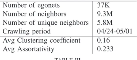
To analyze topological characteristics of the Facebook
population, we collected ∼ 37K egonets that contain basic node information (see Fig 1) for ∼ 5.8M unique neighbors. Table III contains a summary of the egonet dataset, including properties that we analyze in section VI.
Number of egonets 37K
Number of neighbors 9.3M Number of unique neighbors 5.8M
Crawling period 04/24-05/01
Avg Clustering coefficient 0.16
Avg Assortativity 0.233
TABLE III
EGO NETWORKS COLLECTED FOR37KNODES,RANDOMLY SELECTED FROM THE USERS IN THEMHRWDATASET.
Overall, we sampled 11.6 million unique nodes, and ob-served other 172M as their (unsampled) neighbors. This is a very large sample by itself, especially given thatFacebook
had reported having close to 200 million active users during the time of these measurements.
V. EVALUATION OFSAMPLINGTECHNIQUES In this section, we evaluate all candidate crawling tech-niques (namely BFS, RW and RWRW, MHRW), in terms of their efficiency (convergence) and quality (estimation bias). In
Section V-A, we study the convergence of the random walk methods with respect to several properties of interest. We find a burn-in period of 6K samples, which we exclude from each independent crawl. The remaining 75K x 28 sampled nodes is our main sample dataset; for a fair comparison we also exclude the same number of burn-in samples from all datasets. In Section V-B we examine the quality of the estimation based on each sample. In Section V-C, we summarize our findings and provide practical recommendations.
A. Convergence analysis
There are several crucial parameters that affect the conver-gence of a Markov Chain sample. In this section, we study these parameters by (i) applying formal convergence tests and (ii) using simple, yet insightful, visual inspection of the related traces and histograms.
1) Burn-in: For the random walk-based methods, a number of samples need to be discarded to lose dependence on the initial seed point. Since there is a cost for every user we sample, we would like to choose this value using formal convergence diagnostics so as not to waste resources. Here, we apply the convergence diagnostics presented in Section III-E2 to several properties of the sampled nodes and choose as burn-in the maximum period from all tests.
-2 -1.5 -1 -0.5 0 0.5 1 1.5 2 Geweke Z-Score RWRW -2 -1.5 -1 -0.5 0 0.5 1 1.5 2 100 1000 10000 100000 Geweke Z-Score Iterations MHRW
(a) Number of friends
-2 -1.5 -1 -0.5 0 0.5 1 1.5 2 Geweke Z-Score RWRW -2 -1.5 -1 -0.5 0 0.5 1 1.5 2 100 1000 10000 100000 Geweke Z-Score Iterations MHRW (b) Regional network ID
Fig. 4. Geweke z score (0K..81K) for number of friends (top) and regional network affiliation (bottom). Each line shows the Geweke score for each of the 28 parallel walks.
The Geweke diagnostic is applied in each of the 28 walks separately and compares the difference between the first 10%
1 1.1 1.2 1.3 1.4 1.5 R value RWRW Number of friends Regional Network ID Privacy Australia Membership in (0,1) New York Membership in (0,1)
1 1.1 1.2 1.3 1.4 1.5 100 1000 10000 100000 R value Iterations MHRW Number of friends Regional Network ID Privacy Australia Membership in (0,1) New York Membership in (0,1)
Fig. 5. Gelman-Rubin R score (0K..81K) for five different metrics.
and the last 50% of the walk samples. It declares convergence when all 28 values fall in the[−1,1]interval. Fig. 4 presents the results of the Geweke diagnostic for the user properties of node degree and regional network membership. We start at 50 iterations and plot 150 points logarithmically spaced. We observe that after approximately500−2000iterations we have a z-score strictly between[−1,1]. We also see that RWRW and MHRW perform similarly w.r.t. the Geweke diagnostic.
The Gelman-Rubin diagnostic analyzes all the 28 walks at once by summarizing the difference of the between-walk variances and within-walk variances. In Fig. 5 we plot the R score for the following metrics (i) number of friends (or node degree) (ii) networkID (or regional network) (iii) privacy settings Qv (iv) membership in specific regional networks,
namely Australia and New York. The last user property is defined as follows: if the user in iteration i is a member of networkxthen the metric is set to1, otherwise it is set to0. We can see that the R score varies considerably in the initial hundred to thousand iterations for all properties. To pick an example, we observe a spike between iterations 1,000 and 2,000 in the MHRW crawl for the New York membership. This is most likely the result of certain walks getting trapped within the New York network, which is particularly large. Eventually, after 3000 iterations all the R scores for the properties of interest drop below1.02, the typical target value used for convergence indicator.
We declare convergence when all tests have detected it. The Gelman-Rubin test is the last one at 3K nodes. To be even safer, in each independent walk we conservatively discard 6K nodes, out of 81K nodes total. In the remainder of the evaluation, we work only with the remaining 75K nodes per independent chain for RW, RWRW and MHRW.
2) Total Running Time: Another decision we have to make is about thewalk length, excluding the burn-in samples. This length should be appropriately long to ensure that we are at equilibrium. Here, we utilize multiple ways to analyze the collected samples, so as to increase our confidence that the collected samples are appropriate for further statistical analysis.
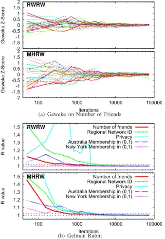
First, we apply formal convergence diagnostics that allow us to assess convergence online by indicating approximate equilibrium. Fig 6 shows the Geweke z-score for the number of
-2 -1.5 -1 -0.5 0 0.5 1 1.5 2 Geweke Z-Score RWRW -2 -1.5 -1 -0.5 0 0.5 1 1.5 2 100 1000 10000 100000 Geweke Z-Score Iterations MHRW
(a) Geweke on Number of Friends
1 1.1 1.2 1.3 1.4 1.5 R value RWRW Number of friends Regional Network ID Privacy Australia Membership in (0,1) New York Membership in (0,1)
1 1.1 1.2 1.3 1.4 1.5 100 1000 10000 100000 R value Iterations MHRW Number of friends Regional Network ID Privacy Australia Membership in (0,1) New York Membership in (0,1)
(b) Gelman Rubin
Fig. 6. Online convergence diagnostics for samples 6K..81K (without burn-in). (top) Geweke z score for number of friends. (bottom) Gelman-Rubin score for five different metrics.
friends (top) and the Gelman-Rubin R score for five different properties (bottom). These results are obtained after discarding the burn-in samples (0K..6K). They show that convergence is attained with at least 3K samples per walk, similar to the section in which we determined the burn-in. This is an indication that the Facebooksocial graph is well connected and our random walks achieved good mixing with our initial selection of random seeds.
Second, we perform visual inspection to check the con-vergence state of our sample by plotting for each walk the running mean of a user property against the iteration number. The intuition is that if convergence has been reached, the running mean of the property will not drastically change as the number of iterations increases. Fig 7 shows for each crawl type the running mean (i) for the node degree in the UNI sample, (ii) in each of the 28 walks individually, and (iii) in an average crawl that combines all 28 walks. It can be seen that in order to estimate the average node degreekv based on
only a single MHRW or RW walk, we should take at least 10K iterations to be likely to get within ±10%off the real value. In contrast, averaging over all 28 walks seems to provide similar or better confidence after fewer than 100 iterations per walk or 100×28∼3K samples over all walks. Additionally, the average MHRW and RW crawls reach stability within 350×28 ∼10K iterations. It is quite clear that the use of multiple parallel walks is very beneficial in the estimation of
0 50 100 150 200 kv MHRW RWRW UNI 28 crawls Average crawl 102 103 104 105 Iterations 100 200 300 400 500 600 kv RW 102 103 104 105 Iterations BFS
Fig. 7. Average node degree kv observed by each crawl, as a function of the number of iterations (or running mean).
user properties of interest.
According to the diagnostics and visual inspection, we need at least 3K samples per walk or3k×28∼84Kover all walks. Since we were not resource constrained during our crawling, we continued sampling users until we reached 81K per walk. One obvious reason is that more samples should decrease the estimation variance. Another reason is that more samples allow us to break the correlation between consecutive samples by thinning the set of sampled users. We use such a thinning process to collect egonets.
3) Thinning: Let us examine the effect of a larger sample on the estimation of user properties. Fig. 8 shows the percent-age of sampled users with specific node degrees and network affiliations, rather than the average over the entire distribution. A walk length of 75K (top) results in much smaller estimation variance per walk than taking 5K consecutive iterations from 50-55K (middle). Fig.8 also reveals the correlation between consecutive samples, even after equilibrium has been reached. It is sometimes reasonable to break this correlation, by con-sidering everyith sample, a process which is calledthinning. The bottom plots in Fig. 8 show 5K iterations per walk with a thinning factor ofi= 10. It performs much better than the middle plot, despite the same total number of samples.
Thinning in MCMC samplings has the side advantage of saving space instead of storing all collected samples. In the case of crawling OSNs, the main bottleneck is the time and bandwidth necessary to perform a single transition, rather than storage and post-processing of the extracted information. Therefore we did not apply thinning to our basic crawls.
However, we applied another idea (sub-sampling), that has a similar effect with thinning, when collecting the second part of our data - the egonets. Indeed, in order to collect the information on a single egonet, our crawler had to visit
10 50 100 200 0.000 0.005 0.010 0.015 0.020 P ( kv = k ) 6k..81k uniform avg of 28 crawls single crawl 10 50 100 200 0.000 0.005 0.010 0.015 0.020 P ( kv = k ) 50k..55k uniform avg of 28 crawls single crawl 10 50 100 200 node degreek 0.000 0.005 0.010 0.015 0.020 P ( kv = k ) 10k..60k with step 10 uniform avg of 28 crawls single crawl
Australia New York, NY India Vancouver, BC
0.000 0.005 0.010 0.015 0.020 P ( N v = N
) 6k..81k uniformavg of 28 crawls
single crawl
Australia New York, NY India Vancouver, BC
0.000 0.005 0.010 0.015 0.020 P ( N v = N
) 50k..55k uniformavg of 28 crawls
single crawl
Australia New York, NY India Vancouver, BC
regional networkN 0.000 0.005 0.010 0.015 0.020 P ( N v = N
) 10k..60k with step 10 uniformavg of 28 crawls
single crawl
Fig. 8. The effect of walk length and thinning on the results. We present histograms of visits at nodes with a specific degreek∈ {10,50,100,200}and network membership (Australia, New York, India, Vancouver), generated under three conditions. (top): All nodes visited after the first 6K burn-in nodes. (middle): 5K consecutive nodes, from hop 50K to hop 55K. This represents a short walk length. (bottom): 5K nodes by taking every 10th sample (thinning).
the user and all its friends, an average ∼ 100 nodes. Due to bandwidth and time constraints, we could fetch only 37K egonets. In order to avoid correlations between consecutive egonets, we collected a random sub-sample of the MHRW (post burn-in) sample, which essentially introduced spacing among sub-sampled nodes.
4) Comparison to Ground Truth: Finally, we compare the random walk techniques in terms of their distance from the true uniform (UNI) distribution as a function of the iterations. In Fig. 9, we show the distance of the estimated distribution from the ground truth in terms of the KL (Kullback-Leibler) metric, that captures the distance of the 2 distributions ac-counting for the bulk of the distributions. We also calculated the Kolmogorov-Smirnov (KS) statistic, not shown here, which captures the maximum vertical distance of two distributions. We found that RWRW is more efficient than MHRW with respect to both statistics. We note that the usage of distance metrics such as KL and KS cannot replace the role of the formal diagnostics which are able to determine convergence online and most importantly in the absence of the ground truth.
5) The choice of metric matters: MCMC is typically used to estimate some user property/metric, i.e.,a function of the underlying random variable. The choice of metric can greatly affect the convergence time. We chose the metrics in the diagnostics, guided by the following principles:
• We chose the node degree because it is one of the metrics we want to estimate; therefore we need to ensure that the MCMC has converged at least with respect to it. The distribution of the node degree is also typically heavy
104 105 106 Iterations 10-3 10-2 10-1 Ku llb ac k-Le ib le r di ve rg en ce RWRW RWRW-Uniq MHRW MHRW-Uniq
Fig. 9. The efficiency of RWRW and MHRW in estimating the degree distribution ofFacebook, in terms of the Kullback-Leibler (KL) divergence. The “Uniq” plots count as iterations only the number of unique sampled nodes, which represents the real bandwidth cost of sampling.
tailed, and thus is slow to converge.
• We also used several additional metrics (e.g. network ID, user ID and membership to specific networks), which are uncorrelated to the node degree and to each other, and thus provide additional assurance for convergence. • We essentially chose to use all the nodal attributes that
were easily and cheaply accessible at each node. These metrics were also relevant to the estimation at later sections.
Let us focus on two of these metrics of interest, namely
node degreeandsizes of geographical networkand study their convergence in more detail. The results for both metrics and all three methods are shown in Fig.10. We expected node degrees to not depend strongly on geography, while the relative size
Australia New York, NY India Vancouver, BC 0.000 0.005 0.010 0.015 0.020 P ( N v = N ) BFS uniform avg of 28 crawls single crawl
Australia New York, NY India Vancouver, BC
0.000 0.005 0.010 0.015 0.020 P ( N v = N ) RW uniform avg of 28 crawls single crawl
Australia New York, NY India Vancouver, BC
0.000 0.005 0.010 0.015 0.020 P ( N v = N ) RWRW uniform avg of 28 crawls single crawl
Australia New York, NY India Vancouver, BC
regional networkN 0.000 0.005 0.010 0.015 0.020 P ( N v = N ) MHRW uniform avg of 28 crawls single crawl 10 50 100 200 0.000 0.005 0.010 0.015 0.020 P ( kv = k ) BFS uniform avg of 28 crawls single crawl 10 50 100 200 0.000 0.005 0.010 0.015 0.020 P ( kv = k ) RW uniform avg of 28 crawls single crawl 10 50 100 200 0.000 0.005 0.010 0.015 0.020 P ( kv = k ) RWRW uniform avg of 28 crawls single crawl 10 50 100 200 node degreek 0.000 0.005 0.010 0.015 0.020 P ( kv = k ) MHRW uniform avg of 28 crawls single crawl
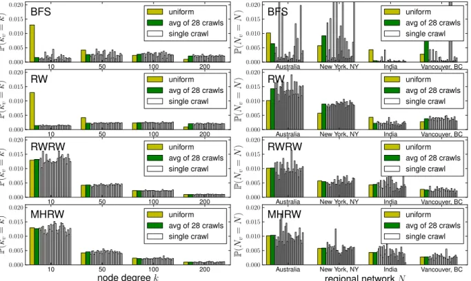
Fig. 10. Histograms of visits at node of a specific degree (left) and in a specific regional network (right). We consider four sampling techniques: BFS, RW, RWRW and MHRW. We present how often a specific type of node is visited by the 28 crawlers (‘crawls’), and by the uniform UNI sampler (‘uniform’). We also plot the visit frequency averaged over all the 28 crawlers (‘average crawl’). Finally, ‘size’ represents the real size of each regional network normalized by the the totalFacebooksize. We used all the 81K nodes visited by each crawl, except the first 6K burn-in nodes. The metrics of interest cover roughly the same number of nodes (about 0.1% to 1%), which allows for a fair comparison.
of geographical networks to strongly depend on geography. This implies that (i) the degree distribution will converge fast to a good uniform sample even if the walk has poor mixing and stays in the same region for a long time; (ii) a walk that mixes poorly will take long time to barely reach the networks of interest, not to mention producing a reliable network size estimate. In the latter case, MHRW will need a large number of iterations before collecting a representative sample.
The results presented in Fig. 10 (bottom) confirm our expectation. MHRW performs much better when estimating the probability of a node having a given degree, than the probability of a node belonging to a specific regional network. For example, one MHRW crawl overestimates the size of “New York, NY” by roughly 100%. The probability that a perfect uniform sampling makes such an error (or larger) is
P∞ i=i0 i n pi(1−p)i ≃4.3·10−13, where we tooki 0 = 1k,
n = 81K and p = 0.006. Even given such single-walk deviations, the multiple-walk average for the MHRW crawl provides an excellent estimate of the true population size.
B. Unbiased Estimation
This section presents the main results of this chapter. First, the MHRW and RWRW methods perform very well: they estimate two distributions of interest (namely node degree, regional network size) essentially identically to the UNI sam-pler. Second, the baseline algorithms (BFS and RW) deviate substantively from the truth and lead to misleading estimates.
10−8 10−7 10−6 10−5 10−4 10−3 10−2 10−1
P
(
k
v=
k
)
MHRW UNI 28 Crawls Average crawl RWRW UNI 28 Crawls Average crawl 100 101 102 103node degree
k
10−8 10−7 10−6 10−5 10−4 10−3 10−2 10−1P
(
k
v=
k
)
RW UNI 28 Crawls Average crawl 100 101 102 103node degree
k
BFS UNI 28 Crawls Average crawlFig. 11. Degree distribution (pdf) estimated by the sampling techniques and the ground truth (uniform sampler). MHRW and RWRW agree almost perfectly with the UNI sample; while BFS and RW deviate significantly. We use log-log scale and logarithmic binning of data in all plots.
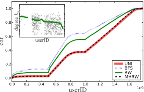
0.0 0.2 0.4 0.6 0.8 1.0 1.2 1.4 1.6 1e9 0.0 0.2 0.4 0.6 0.8 1.0 UNI BFS RW MHRW d eg re e kv userID userID cd f
Fig. 12. User ID space usage discovered by BFS, RW, MHRW and UNI. Each user is assigned a 32 bit long userID. Although this results in numbers up to4.3e9, the values above1.8e9almost never occur. Inset: The average node degree (in log scale) as a function of userID.
1) Node degree distribution: In Fig. 11 we present the degree distributions estimated by MHRW, RWRW, RW, and BFS. The average MHRW crawl’s pdf, shown in Fig. 11(a) is virtually identical to UNI. Moreover, the degree distribution found by each of the 28 chains separately are almost identical. In contrast, RW and BFS shown in Fig. 11(c) and (d) introduce a strong bias towards the high degree nodes. For example, the low-degree nodes are under-represented by two orders of magnitude. As a result, the estimated average node degree is kv ≃ 95 for MHRW and UNI, and kv ≃ 330 for BFS
and RW. Interestingly, this bias is almost the same in the case of BFS and RW, but BFS is characterized by a much higher variance. Notice that that BFS and RW estimate wrong not only the parameters but also the shape of the degree distribution, thus leading to wrong information. Re-weighting the simple RW corrects for the bias and results to RWRW, which performs almost identical to UNI, as shown in 11(b). As a side observation we can also see that the true degree distribution clearlydoes notfollow a power-law.
2) Regional networks: Let us now consider a geography-dependent sensitive metric, i.e., the relative size of regional networks. The results are presented in Fig. 10 (right). BFS performs very poorly, which is expected due to its local coverage. RW also produces biased results, possibly because of a slight positive correlation that we observed between network size and average node degree. In contrast, MHRW and RWRW perform very well albeit with higher variance, as already discussed in Section V-A5.
3) The userID space: Finally, we look at the distribution of a property that is completely uncorrelated from the topology of Facebook, namely the user ID. When a new user joins
Facebook, it is automatically assigned a 32-bit number, called userID. It happens before the user specifies its profile, joins networks or adds friends, and therefore one could expect no correlations between userID and these features. In other words, the degree bias of BFS and RW should not affect the usage of userID space. Therefore, at first, we were surprised to find big differences in the usage of userID space discovered by BFS, RW and MHRW. We present the results in Fig 12.
Note that the userID space is not covered uniformly, prob-ably for historical reasons. BFS and RW are clearly shifted
towards lower userIDs. The origin of this shift is probably historical. The sharp steps at 229≃0.5e9 and at 230≃1.0e9
suggest thatFacebookwas first using only 29 bit of userIDs, then 30, and now 31. As a result, users that joined earlier have the smaller userIDs. At the same time, older users should have higher degrees on average, which implies that userIDs should be negatively correlated with node degrees. This is indeed the case, as we show in the inset of Fig 12.9 This, together with
the degree bias of BFS and RW, explains the shifts of userIDs distributions observed in the main plot in Fig 12. In contrast to BFS and RW, MHRW performed extremely well with respect to the userID metric.
C. Findings and Practical Recommendations
1) Choosing between methods: First and most important, the above comparison demonstrates that both MHRW and RWRW succeed in estimating several Facebook properties of interest virtually identically to UNI. In contrast, commonly used baseline methods (BFS and simple RW) fail,i.e.,deviate significantly from the truth and lead to substantively erroneous estimates. Moreover, the bias of BFS and RW shows up not only when estimating directly node degrees (which was expected), but also when we consider other metrics seemingly uncorrelated metrics (such as the size of regional network), which end up being correlated to node degree. This makes the case for moving from “1st generation” traversal methods such as BFS, which have been predominantly used in the measurements community so far [9,12,13], to more principled, “2nd generation”, sampling techniques whose bias can be analyzed and/or corrected for. The random walks considered in this paper, RW, RWRW and MHRW, are well-known in the field of Monte Carlo Markov Chains (MCMC). We apply and adapt these methods toFacebook, for the first time, and we demonstrate that, when appropriately used, they perform remarkably well on real-world OSNs.
2) Adding convergence diagnostics and parallel crawls:
A key ingredient of our implementation - to the best of our knowledge, not previously employed in network sampling -was the use of formal online convergence diagnostic tests. We tested these on several metrics of interest within and across chains, showing that convergence was obtained within a reasonable number of iterations. We believe that such tests can and should be used in field implementations of walk-based sampling methods to ensure that samples are adequate for subsequent analysis. Another key ingredient of our imple-mentation was the use of independent crawlers (started from several random independent starting points, unlike [17,19] who use a single starting point), which both improved convergence and decreased the duration of the crawls.
9Our observations are also confirmed by internal sources withinFacebook [65]. According to them,Facebook’s user ID assignment reflects the history of the website and has transitioned through several phases. Initially, userIDs were auto-incremented starting at 4. As more networks, such as colleges or high schools, were supported, customized userID spaces were assigned per college i.e., Stanford IDs were assigned between 200000-299999. Finally, open registration to all users introduced scalability problems and made userID assignment less predictable.