performance management
Gabriele Kotsis, Martin Pinzger
Department of Telecooperation, Johannes Kepler University, Altenberger Str. 69, 4040 Linz, Austria
[email protected], [email protected]
Abstract. The growing demand for quality and performance has be-come a discriminating factor in the field of software applications. Specif-ically in the area of web applications, performance has become a key fac-tor for success creating the need for new types of performance evaluation models and methods capable of representing the dynamic characteristics of web environments.
In this paper we will recall seminal work in this area and present AWPS, a tool for automatic web performance simulation and prediction. AWPS is capable of (a) automatically creating a web performance simulation and (b) conducting trend analysis of the system under test. The operation and usage of this tool is demonstrated in a case study of a two-tier architecture system.
Keywords: Web Performance, Simulation, Automation
1
Introduction and Related Work
Today, performance represents the key to successful applications, especially in the field of web applications. In new software projects, performance aspects are often already part of the development process [6], yet there are still many projects where performance aspects have not been considered and the number of realizable improvements are limited.
The traditional approach to evaluate the performance of computer systems and networks is an “off-line” performance analysis cycle (see for example [11]). Starting with a characterisation of the system under study and a characteri-sation of the load, a performance model is built and performance results are obtained by applying performance evaluation techniques (including analytical, numerical, or simulation techniques). Alternatively, performance measurements of the real system can replace the modelling and evaluation step. In any case, an interpretation of results follows which can trigger either a refinement of the model (or new measurements) if the results do not provide the required insight, or which will lead to performance tuning activities (system side or load side) if performance deficiencies are detected.
It follows quite natural (and has been observed in the history of performance evaluation, see for example the report given in [8]) that changes in the com-puting environment (parallel and distributed comcom-puting, network comcom-puting,
mobile computing, pervasive computing, etc.) and new system features (security and reliability mechanisms, agent-based systems, intelligent networks, adaptive systems, etc.) pose new challenges to performance evaluation by raising the need for new analysis methodologies.
From a load modelling point of view, the difference in using computing re-source has changed the type of model for workload characterization. While in the early days of computing (70s) the typical systems were used in batch or interactive mode, static workload models [4] could adequately represent the user behaviour. In the 80s, dynamic workload models were introduced, which were able to represent variabilities in user behavior ([1, 5]). In the 90s, generative workload models [3, 17] have been proposed as a suitable method for bridging the gap between the user’s application oriented view of the load and the actual load (physical, resource oriented requests) submitted to the system. Hierarchical descriptions of workloads have proven their usability for representing workloads of parallel and distributed systems [7, 18, 2], or web traffic characterisation [13]. But the many aspects of emerging computing environments create a vari-ety of performance influencing factors which cannot be adequately represented in a model. Applications in such environments are typically characterised by a complex, irregular, data-dependent execution behavior which is highly dynamic and has time varying resource demands. The performance delivered by the exe-cution platform is hard to predict as it is usually constituted of heterogeneous components.
In addition, a demand is observed for immediate, embedded performance tuning actions replacing the traditional off-line approach of performance anal-ysis. The human expert driven process of constructing a model, evaluating it, validating and interpretating the results and finally putting performance tun-ing activities into effect is no longer adequate if real-time responsiveness of the system is needed.
Therefore we follow an on-line, dynamic performance management approach as outlined in [12]. Several approaches have been proposed to support an auto-mated performance evaluation and prediction, see for example [14, 10, 19], but only a few presenting fully integrated frameworks such as [21].
In this paper we demonstrate this general concept of performance manage-ment in web based information systems. The paper is separated into two main parts. First AWPS, a framework for automated web performance simulation and prediction, will be described, then a case study dealing with the two-tier architecture system will be presented.
Finally conclusions based on the case study will be drawn and from these, the next necessary steps will be derived.
2
AWPS Concept
With AWPS a system which is capable of automatically creating a web per-formance simulation and conducting a trend analysis of the SUT is presented [15]. The concept of AWPS is based on building a system which enables system
administrators with little experience in the field of web performance simulation and prediction to analyze and monitor their system. The basic concept is to integrate the AWPS into the SUT in a transparent and non-intrusive way. From the three key functions of AWPS,data collection, simulation and prediction, only the datacollection part needs to be integrated into the SUT. The simulation and prediction component provide the user access to the system from an observer point of view, requiring no specific experiences in simulation or prediction.
2.1 Data Collection Component
The data collection component is made up of three elements which are the configuration component, the data recording component and the monitoring component. The configuration component provides access to static information about the SUT.
The task of the data recording component is to store and pre-process the collected information about the SUT, key features here are: capability to serve several components at the same time(multi-threaded / multi-processor), to pro-videhigh performance access to the stored data and toincrementally add data.
The monitoring component provides the input interface to the SUT, for its realisation software monitoring [11] is used. Thereby three types based on their interaction with the environment are distinguished, active, passive and active & passive software monitoring. All three supported types are described in detail in [15], by default the passive software monitoring approach (e.g. network sniffing) is used, as it has no influence on the SUT.
2.2 Simulation Component
The simulation component represents a core component of the AWPS. The func-tions of this component are quite demanding concerning system resources and time. Therefore a key requirement for the so calledon-line simulationis that the time required for the simulation, must not be higher than the real response time of the system. In the following subsections a description of the subcomponents is given.
Model Generation Component
The model generation component deals with the task of initially generating the simulation model. For this the component depends on the information provided by the data collection component. To accomplish this task, two solution types could be used in principle. These types are:
1. Minimum complexity simulation model: The idea is to start with the simplest possible simulation model, in case of queuing-network-models this would be a single class / single queue / single server model.
2. Maximum complexity simulation model: In a maximum complexity simula-tion model the system starts with a simulasimula-tion model, which attempts to
include all possible combinations at startup. An example for this could be a queuing-network-model which is initialized with a multi class / multi queue / multi server model.
Currently, the AWPS uses themaximum complexity simulation model strategy, with the constraint that at least one monitoring point per server is provided.
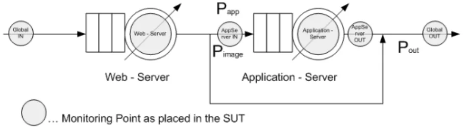
As example for the simulation model generation process two examples with four monitoring points are provided. The first example is a system with a web server and an application server, the second example is a system with a web server, an application server and a database server. The basic monitoring points Global In and Global Out were placed at the Input and Output of the system, additonally one monitoring point was placed at theApplication Server Input.
In the first example the fourth monitoring point is the Application Server Out inserted before the Global Out, by the AWPS the following formula are generated and used for the calculation of the request delay time.
T otalSystemT ime=GlobalOut−GlobalIn (1)
W ebServerT imeA=AppServerIn−GlobalIn (2)
AppServerT ime=AppServerOut−AppServerIn (3)
W ebServerT imeB=GlobalOut−AppServerOut (4)
W ebServerT ime=W ebServerT imeA+W ebServerT imeB (5) Based on this a simulation model as shown in Figure 1 is created. In this case it consists of two servers, two queues supporting multiple classes.
Fig. 1.Generated Simulation Model with 4 Monitoring Points
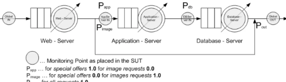
In the second example the fourth monitoring point is theDatabase Server In placed at the Database Server Input / at the Application Server Output. The following formula are generated and used for calculation by the AWPS.
T otalSystemT ime=GlobalOut−GlobalIn (6)
AppServerT ime=DBServerIn−AppServerIn (8)
DBServerT ime=GlobalOut−DBServerIn (9) In this case the setup would lead to a simulation model with three servers and three queues supporting multiple classes, as shown in Figure 2.
Fig. 2.Generated Simulation Model with 4 Monitoring Points (database server)
Model Comparison Component
To be able to determine whether to execute the model adjustment component or to keep the simulation model as it is, it is necessary to compare the results of the simulation model with the results of the SUT. For this the model comparison component uses on the one hand the monitoring information provided by the data collection component and on the other hand the results generated by the model simulation component which executes the simulation model.
The comparison process is structured in the following way. When a request is sent to the SUT, it is also inserted into the simulation model. Then the response should be created with the same time delay by the SUT and the simulation model. If there is a discrepancy (error) which is higher than the acceptable value, the simulation model needs to be adjusted.
Model Adjustment Component
The model adjustment component has several options to adjust the simulation model of the SUT. Depending on the performance of the simulation observed by the model comparison component, parameter changes (e.g. delay of a server) are applied or strategies are changed. The option to change a configuration value of the simulation model should be observed more closely. Four strategies for estimating the correct parameters for a link (server delay) in the simulation model should be mentioned: AVG strategy, median strategy, ARMA strategy and ARMA with 60 sec. grouping strategy [16].
Model Simulation Component
the simulation model. As already mentioned for the AWPS it is very important to have a simulation which is at least as fast as the SUT to work properly. Given the demands it is the goal to create a model simulation component which is independent from a basic simulation environment, to be able to replace the simulation environment if the performance demands are not fulfilled. At the cur-rent state of the AWPS the JSIM [9] simulation framework is used as simulation environment.
2.3 Prediction Component
The prediction component is separated into four components, these are: the sta-tistical component, the scenario generation & execution component, the longterm analysis component and reporting component.
The task of thisStatistical Component is to provide a statistical analysis of the data provided by the data collection component. This analysis includes ba-sic statistical information about the SUT, like for example min/max/mean/avg response time, min/max/mean/avg utilization, number of requests and number of errors.
TheScenario Generation & Execution Componentuses the simulation model to execute generated scenarios and test for possible events which could occur in the SUT. Results provided by these experiments are reported back to the data collection component.
The basis for theLongterm Analysis Component is the information provided by the data collection component, the results from the scenario generation & execution component are of special importance. This information is processed and analyzed, to identify trends for the SUT concerning the perspective of avail-ability and service level agreement.
TheReporting Component is intended as a base for the conversion of data which should be shared with the environment of the AWPS. To accomplish this, the reporting component has to provide a high flexibility and a suitable set of communication interfaces.
3
AWPS Environment Interaction
In this section the interaction of the AWPS with its environment is described. Especially information concerning the current development status of the AWPS and resulting limitations or simplifications are provided. In general there are two areas to deal with, the system setup where the components setup, which was used during the case study is described and the influence of the AWPS on the SUT.
3.1 System Setup
The AWPS is installed on a separate system which has been placed in the same network segment (collision domain) as the SUT, as a consequence the passive
software monitoring strategy can be used. For the case study a multi class / single queue / multi server model is created, by the system, additional informations about the parameters can be found in [16].
The prediction component is integrated in a basic version so that, it is pos-sible to evaluate the results and compare the predictions with the actually oc-curred events. The data recording component is fully integrated, for evaluation purposes a development feature which provides pre-recorded data is used.
3.2 Influence of the AWPS on the Productive System
The influence of the AWPS on the SUT is given by the overhead produced by the monitoring method and the additional network traffic coming from the effort to transfer the monitored information to the AWPS (data collection component). The AWPS setup used in the case study presented in section 4, does not influence the SUT since only passive software monitoring is used.
4
Case Study
The case study was done on a two tier web application, which provides as func-tionality a web page where you can search and book space flights. The SUT represents a fully operable environment which was developed by a company to illustrate their product. For proprietary reasons it cannot be referenced directly. The system uses a JSP front-end (41 JSP-Files) and a Web Service as back-end (30 Class-Files), in the following sections at first the system environment and then the detailed objectives of the case study are described. Then the used set-tings and the simulation model which is generated by the AWPS are presented, finally the results of the case study are discussed.
4.1 System Environment
The system environment for the two tier web application consists of a back-end system and a front-end system.
For the back-end system an Intel Core Duo with 2.20 GHz and 2 GB RAM with Microsoft Windows XP and Service Pack 2 was used. The front-end system was an Intel Centrino with 1.60 GHz and 1 GB RAM with Microsoft Windows XP and Service Pack 3. As web server for the front-end and as application server for the back-end the JBOSS in version 4.2.3 was used. The connection between the front-end system and the back-end system was established via a direct 100 Mbit Ethernet Network connection.
For the AWPS as platform an Intel Centrino with 1.60 GHz and 1 GB RAM with a Microsoft Windows XP with Service Pack 3, a PostgreSQL 8.3 database, Mathematica 5.2 and a WampServer 2.0 were used. The monitoring of the two tier web application was done by passive software monitoring as described in section 4.3.
4.2 Objectives of the Case Study
The objective of the case study is to provide an insight into the AWPS and to prove the simulation model generation process is feasible. Additionally the dif-ferent integrated strategies used for simulation model adjustments are evaluated.
4.3 Case Study Settings
The case study settings can be separated in three parts on the system load generation, theAWPS configuration and themonitoring configuration.
At first thesystem load generation should be specified, the artificial system load for the case study was realized using the Microsoft Web Application Stress 1.1 Tool [20]. The tool was configured to send requests to the system requesting 12 different web pages, in the time frame of an hour 69621 request were sent.
Secondly themonitoring configuration should be provided, as mentioned in the system environment section, passive software monitoring was used. The mon-itoring was done on three points:
1. Web Server In / Global In, this monitoring point represents the first of the two minimal required monitoring points. In this and in the common case this monitoring point is realized by the capturing of the traffic (requests) sent to the web server.
2. Application Server In, based on this monitoring point the AWPS can deter-mine that more than one server is used. Additionally the distribution of the response time between the front-end and the back-end can be determined. 3. Web Server Out / Global Out, this monitoring point represents the second
of the two minimal required monitoring points. As theGlobal Inmonitoring point it captures the messages sent between the server and the client, in this case the response message (HTTP) is captured.
Finally the AWPS configuration is provided for the 12 executed test cases: The four model adjustment strategies (AVG strategy, Median strategy, ARMA strategy, ARMA with 60 sec. Grouping strategy) were evaluated with step size of 1000, 100 and 10. With the step size the number of request considered by the system before reevaluating the configuration of the AWPS is meant. This value also defines the number of request which are predicted by the AWPS. Additionally the system was configured to support multiple classes of requests, in concrete the requests for images (GIF) and the requests for sites which require a query for special offers (do?action=special) in the back-end were considered. It should be stated that the specification of the considered request types is optional, if no information is provided the system learns the request types automatically. Predefined values of the AWPS configuration which were used during the evaluation are aAVG Strategy Windows Size of 5000, aMedian Strategy Position in percent of 50 and apMax and qMax of 5 for the ARMA and ARMA with 60 sec. grouping Strategy.
4.4 Generated Simulation Model
The generated simulation model is based on the AWPS configuration and on the information provided by the monitoring points. The three monitoring points listed in section 4.3 are used to calculate a request delay time for the SUT auto-matically, the following formula illustrate this (no user interaction is required).
T otalSystemT ime=GlobalOut−GlobalIn (10)
W ebServerT ime=AppServerIn−GlobalIn (11)
AppServerT ime=GlobalOut−AppServerIn (12) This calculation is done for each request class, out of this the time consumption for the images (GIF) turns out to be zero for the Application Server. This is interpreted by the system and results in the conclusion that the images (GIF) request do not need the Application Server they only require the Web Server. For the special offers (do?action=special) request the system returns a time for the Web Sever and the Application Server which is interpreted accordingly.
Based on this request delay time structure a similar simulation model as shown in Figure 1 is created automatically. Only the indicated monitoring point AppServer Out is not included, as this monitoring point is not configured in the system setup (section 4.3).
4.5 Case Study Results
The data can be separated into three parts, the calculation time consumption, the comparison for significant differences between simulated and reference data and the comparison of the delta error between the integrated simulation model adjustment strategies.
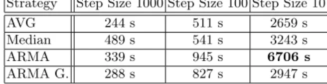
Thecalculation time consumption consists of the total time required for the system to generate, adjust and execute the simulated model. The periods in which the AWPS was idle waiting for new requests is not included. Out of these a calculation time for the different integrated adjustment strategies for the 60 minutes case study can be provided, see Table 1. The results shown in the table show that with reducing the step size the calculation time increases, however for all methods for a step size of 1000 and 100 the time consumption is below 60 minutes so that means that the system is online capable. For a step size of 10 the system shows problems with the ARMA strategy. These limitations can be solved by additional hardware. Preliminary test results indicate that an Intel Dual Core with 2.4 Ghz and 2GB of RAM is already sufficient.
Thesignificant difference between simulation and reference data, is evaluated with a double sided t-Test with a threshold of 5 percent between the results. In Table 2 these results are presented and indicate that the differences are not significant for the special offers (do?action=special) request class for a step size of 1000 for the AVG, ARMA and ARMA G. method. There is no significant difference for a step size of 100 and 10 for the ARMA. However a significant difference in the image (GIF) request class is given. The reason for this is that
Strategy Step Size 1000 Step Size 100 Step Size 10
AVG 244 s 511 s 2659 s
Median 489 s 541 s 3243 s
ARMA 339 s 945 s 6706 s
ARMA G. 288 s 827 s 2947 s
Table 1.Calculation time consumption. Values below 3600 sec. mean that the adjust-ment method is online-capable.
the difference in the response time of the request class is different to the special offers (do?action=special) request class response time by a factor of 1000. The cacheing strategies of the simulated server differ in this special case too much from the cacheing strategies of the web server of the SUT. If only the image (GIF) request class or a slow image (GIF) request class is considered the difference between the SUT and the simulates system again is not significant, because the influence of the right chasing strategy on the server is reduced. The significant
Strategy Step Size 1000 Step Size 100 Step Size 10 image special image special image special AVG Yes. No (0.980230) Yes Yes (0.935309) Yes Yes (0.789822) Median Yes. Yes (0.758424) Yes Yes (0.335950) Yes Yes (0.002655) ARMA Yes. No (0.982876) Yes No (0.990521) Yes No (0.998247) ARMA G. Yes. No (0.992849) Yes Yes (0.289593) Yes Yes (0.000000) Table 2. Significant difference between simulation and reference data. The value in the brackets represents the double sided t-Test value.
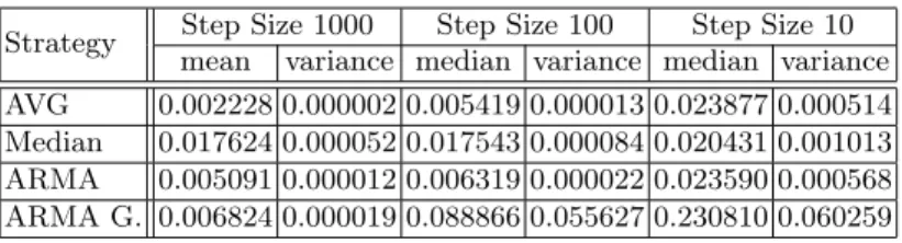
difference in the delta error of the integrated simulation adjustment method, meaning the absolute value of the error between the simulated values and the measured values is analyzed with a two sided t-Test with a threshold of 5 percent. The analysis is done to determine if there is a significant difference between the integrated adjustment strategies. The results clearly indicate that the ARMA strategy provides the best results for all step sizes, the difference between ARMA and ARMA G. is minimal at a step size of 1000 but still significant. For a step size of 10 the t-Test indicates the AVG method is the best approximation, however the difference is still significant. In Table 3 the mean values and the variance values of the integrated simulation adjustment methods are presented to provide some insight concerning the range of the values, keeping in mind the values, reference to the delta error and the fact that reducing the step size also means that the smoothing effect by the average calculation is reduced.
Strategy Step Size 1000 Step Size 100 Step Size 10 mean variance median variance median variance AVG 0.002228 0.000002 0.005419 0.000013 0.023877 0.000514 Median 0.017624 0.000052 0.017543 0.000084 0.020431 0.001013 ARMA 0.005091 0.000012 0.006319 0.000022 0.023590 0.000568 ARMA G. 0.006824 0.000019 0.088866 0.055627 0.230810 0.060259
Table 3.Mean values and Variance values in seconds referring to the delta error, for the special offers (do?action=special) request class
5
Conclusion
As demonstrated by the case study, AWPS works as expected and provides repre-sentative results. The simulation model generation process works autonomously and is sufficiently fault-tolerant. The integrated strategies for the adjustment of the simulation model work accurately, especially when the autoregressive moving average (ARMA) model strategy is used. The AWPS provides suitable results not only for artificial systems shown in [16], it also provides representative results for a productive system, as demonstrated with this case study.
The known limitation of the AWPS is that at least two monitoring points are required and that for each server which should be considered in the simulation at least one monitoring point is required, two monitoring points per server ensure accurate and reliable results as presented in the case study but at the costs of slightly higher level of intrusion.
Nevertheless, improvements of the AWPS are necessary in two ways: the functionality should be enhanced (e.g. adaptive scenario generation), and addi-tional case studies need to be done, including the analysis of a productive system under high (real) load.
References
1. M. Calzarossa, M. Italiani, and G. Serazzi. A Workload Model Representative of Static and Dynamic Characteristics. Acta Informatica, 23:255–266, 1986.
2. Maria Calzarossa, Alessandro P. Merlo, Daniele Tessera, G¨unter Haring, and Gabriele Kotsis. A hierarchical approach to workload characterization for parallel systems. InHPCN Europe, pages 102–109, 1995.
3. Q. Dulz and S. Hofman. Grammar-based workload modeling of communication systems. InProc. of Intl. Conference on Modeling Techniques and Tools For Com-puter Performance Evaluation, Tunis, 1991.
4. D. Ferrari. Workload Characterization and Selection in Computer Performance Measurement. Computer, 5(4):18–24, 1972.
5. G. Haring. On Stochastic Models of Interactive Workloads. In A.K. Agrawala and S.K. Tripathi, editors,PERFORMANCE ’83, pages 133–152. North-Holland, 1983.
6. G. Haring and A. Ferscha. Performance oriented development of parallel software with capse. In Proceedings of the 2nd Workshop on Environments and Tools for Parallel Scientific Computing. SIAM, 1994.
7. G. Haring and Gabriele Kotsis. Workload modeling for parallel processing systems. In P. Dowd and E. Gelenbe, editors,MASCOTS’95, Proc. of the 3rd Int. Work-shop on Modeling, Analysis and Simulation of Computer and Telecommunication Systems, pages 8–12. IEEE Computer Society Press, 1995. ISBN 0-8186-6902-0. (invited Paper).
8. G. Haring, Ch. Lindemann, and M. Reiser, editors. Performance Evaluation of Computer Systems and Communication Networks. Dagstuhl-Seminar-Report, No 189, 1997.
9. Jennifer Hou. J-sim official, January 2005.
http://sites.google.com/site/jsimofficial/.
10. Tauseef A. Israr, Danny H. Lau, Greg Franks, and Murray Woodside. Automatic generation of layered queuing software performance models from commonly avail-able traces. InWOSP ’05: Proceedings of the 5th international workshop on Soft-ware and performance, pages 147–158, New York, NY, USA, 2005. ACM.
11. Raj Jain. The Art of Computer Systems Performance Analysis, pages 93–110. John Wiley and Sons, Inc., 1991.
12. Gabriele Kotsis. Performance management in dynamic computing environments. In Maria Carla Calzarossa and Erol Gelenbe, editors,Performance Tools and Ap-plications to Networked Systems, pages 254–264. Springer, LNCS 2965, 2004. ISBN 3-540-21945-5.
13. Gabriele Kotsis, K. Krithivasan, and S.V. Raghavan. Generative workload models of internet traffic. InProceedings of the ICICS Conference, Singapore, pages 152– 156. IEEE Singapore, 1997.
14. Adrian Mos and John Murphy. A framework for performance monitoring, mod-elling and prediction of component oriented distributed systems. In WOSP ’02: Proceedings of the 3rd international workshop on Software and performance, pages 235–236, New York, NY, USA, 2002. ACM.
15. Martin Pinzger. Automated web performance analysis. InASE, pages 513–516. IEEE, 2008.
16. Martin Pinzger. Strategies for automated performance simulation model adjust-ment, preliminary results. In Workshop on Monitoring, Adaptation and Beyond (MONA+) at the ServiceWave 2008 Conference. Universitt Duisburg-Essen, ICB-Research Report No. 34, 2009.
17. S. V. Raghavan, D. Vasuki Ammaiyar, and G¨unter Haring. Generative networkload models for a single server environment. InSIGMETRICS, pages 118–127, 1994. 18. S. V. Raghavan, D. Vasuki Ammaiyar, and G¨unter Haring. Hierarchical approach
to building generative networkload models. Computer Networks and ISDN Sys-tems, 27(7):1193–1206, 1995.
19. Pere P. Sancho, Carlos Juiz, and Ramon Puigjaner. Automatic performance eval-uation and feedback for mascot designs. In WOSP ’05: Proceedings of the 5th international workshop on Software and performance, pages 193–194, New York, NY, USA, 2005. ACM.
20. Microsoft AppCenter Service Team. Microsoft web application stress 1.1, 1999. http://webtool.rte.microsoft.com/.
21. Li Zhang, Zhen Liu, Anton Riabov, Monty Schulman, Cathy H. Xia, and Fan Zhang. A comprehensive toolset for workload characterization, performance mod-eling, and online control. InComputer Performance Evaluation / TOOLS, pages 63–77, 2003.