Multistage stochastic programming: A scenario tree based approach to planning under uncertainty

A Scenario Tree Based Approach

to Planning under Uncertainty

Boris Defourny, Damien Ernst, and Louis Wehenkel University of Li`ege, Systems and Modeling, B28,

B-4000 Li`ege, Belgium

{Boris.Defourny,dernst,L.Wehenkel}@ulg.ac.be

Abstract. In this chapter, we present the multistage stochastic pro-gramming framework for sequential decision making under uncertainty and stress its differences with Markov Decision Processes. We describe the main approximation technique used for solving problems formulated in the multistage stochastic programming framework, which is based on a discretization of the disturbance space. We explain that one issue of the approach is that the discretization scheme leads in practice to ill-posed problems, because the complexity of the numerical optimization algo-rithms used for computing the decisions restricts the number of samples and optimization variables that one can use for approximating expecta-tions, and therefore makes the numerical solutions very sensitive to the parameters of the discretization. As the framework is weak in the ab-sence of efficient tools for evaluating and eventually selecting competing approximate solutions, we show how one can extend it by using machine learning based techniques, so as to yield a sound and generic method to solve approximately a large class of multistage decision problems un-der uncertainty. The framework and solution techniques presented in the chapter are explained and illustrated on several examples. Along the way, we describe notions from decision theory that are relevant to sequential decision making under uncertainty in general.

1

INTRODUCTION

This chapter addresses decision problems under uncertainty for which complex decisions can be taken in several successive stages. By complex decisions, it is meant that the decisions are structured by numerous constraints or lie in high-dimensional spaces. Problems where this situation arises include capacity plan-ning, production planplan-ning, transportation and logistics, financial management, and others (Wallace & Ziemba, 2005). While those applications are not currently mainstream domains of research in artificial intelligence, where many achieve-ments have already been obtained for control problems with a finite number of actions and for problems where the uncertainty is reduced to some independent noise perturbing the dynamics of the controlled system, the interest for applica-tions closer to operaapplica-tions research — where single instantaneous decisions may already be hard to find and where uncertainties from the environment may be delicate to model — and for applications closer to those addressed in decision theory — where complex objectives and potentially conflicting requirements have

2

to be taken into account — seems to be growing in the machine learning commu-nity, as indicated by a series of advances in approximate dynamic programming motivated by such applications (Powell, 2007; Cs´aji & Monostori, 2008).

Computing strategies involving complex decisions calls for optimization tech-niques that can go beyond the simple enumeration and evaluation of the possible actions of an agent. Multistage stochastic programming, the approach presented in this chapter, relies on mathematical programming and probability theory. It has been recognized by several industries — mainly in energy (Kallrath, Parda-los, Rebennack, & Scheidt, 2009) and finance (Dempster, Pflug, & Mitra, 2008) — as a promising framework to formulate complex problems under uncertainty, exploit domain knowledge, use risk-averse objectives, incorporate probabilistic and dynamical aspects, while preserving structures compatible with large-scale optimization techniques.

Even for readers primarily concerned by robotics, the development of these techniques for sequential decision making under uncertainty is interesting to follow: Puterman (1994), citing Arrow (1958) on the early roots of sequential decision processes, recalls the role of the multi-period inventory models from the industry in the development of the theory of Markov Decision Processes (Chapter 3 of this book); we could also mention the role of applications in finance as a motivation for the early theory of multi-armed bandits and for the theory of sequential prediction, now an important field of research in machine learning.

The objective of the chapter is to provide a functional view of the concepts and methods proper to multistage stochastic programming.

To communicate the spirit of the approach, we use examples that are short in their description. We use the freely available optimization software cvx (Grant & Boyd, 2009), which has the merit of enabling occasional users of optimiza-tion techniques to conduct their own numerical experiments in Matlab (The MathWorks, Inc., 2004).

We cover our recent contributions on scenario tree selection and out-of-sample validation of optimized models (Defourny, Ernst, & Wehenkel, 2009), which suggest partial answers to issues concerning the selection of approxima-tions/discretization of multistage stochastic programs, and to issues concerning the efficient comparison among those approximations.

Many details relative to optimization algorithms and specific problem classes have been left aside in our presentation. A more extensive coverage of these aspects can be found in J. Birge and Louveaux (1997); Shapiro, Dentcheva, and Ruszczy´nski (2009). These excellent sources also present many examples of formulations of stochastic programming models. Note, however, that there is no such thing as a general theory on multistage stochastic programming that would allow the many approximation/discretization schemes proposed in the technical literature (referenced later in the chapter) to be sorted out.

Background

Now, even if we insist on concepts, our presentation cannot totally escape from the fact that multistage stochastic programming uses optimization techniques from mathematical programming, and can harness advances in the field of opti-mization.

To describe what a mathematical program is, simply say that there is a function F, called the objective function, that assigns to x _∈ X a real-valued

costF(x), that there exists a subsetCofX, called the feasibility set, describing admissible points x(by functional relations, not by enumeration), and that the program formulates our goal of computing the minimal value ofF onC, written minCF, and a solutionx∗ ∈ C attaining that optimal value, that is, F(x∗) = minCF. Note that the set of pointsx∈Csuch thatF(x) = minCF, called the optimal solution set and written argminCF, need not be a singleton. Obviously, many problems can be formulated in that way, and what makes the interest of optimization theory is the clarification of the conditions onF andC that make a minimization problem well-posed (minCF finite and attained) and efficiently solvable. For instance, in the chapter, we speak of convex optimization problems. To describe this class, imagine a point ¯x_∈C, and assume that for eachx_∈C in a neighborhood of ¯x, we haveF(x)≥F(¯x). The class of convex problems is a class for which any such ¯xbelongs to the optimal solution set argminCF. In particular, the minimization of F overC with F an affine function ofx∈ Rn

(meaning that F has values F(x) = Pni=1aixi +a0) and C = {x : gi(x) ≤ 0, hj(x) = 0 for i∈I, j∈J}for some index setsI,J and affine functionsgi,hj, turns out to be a convex problem (linear programming) for which huge instances — in terms of the dimension ofxand the cardinality ofI,J — can be solved. Typically, formulation tricks are used to compensate the structural limitations onF,C by an augmentation of the dimension ofxand the introduction of new constraints gi(x)≤0,hj(x) = 0. For example, minimizing the piecewise linear function f(x) = max_{aix+bi : i∈ I} defined on x∈R, with I ={1, . . . , m} andai, bi∈R, is the same as minimizing the linear functionF(x, t) =tover the setC=_{(x, t)_∈R×R:aix+bi−t≤0, i∈I}. The trick can be particularized tof(x) =|x|= max{x,−x}.

For more on applied convex optimization, we refer to Boyd and Vandenberghe (2004). But if the reader is ready to accept that conditions on F and C form well-characterized classes of problems, and that through some modeling effort one is often able to formulate interesting problems as an instance of one of those classes, then it is possible to elude a full description of those conditions.

Stochastic programming (Dantzig, 1955) is particular from the point of view of approximation and numerical optimization in that it involves a representation of the objective F by an integral (as soon as F stands for an expected cost under a continuous probability distribution), a large, possibly infinite number of dimensions forx, and a large, possibly infinite number of constraints for defining the feasibility setC. In practice, one has to work with approximationsF0

,C0

, and be content with an approximate solutionx0

∈argminC0F

0

. Multistage stochastic programming (the extension of stochastic programming to sequential decision making) is challenging in that small imbalances in the approximation can be amplified from stage to stage, and thatx0

may be lying in a space of dimension considerably smaller than the initial space for x. Special conditions might be required for ensuring the compatibility of an approximate solution x0

with the initial requirementx_∈C.

One of the main messages of the chapter is that it is actually possible to make use of supervised learning techniques (Hastie, Tibshirani, & Friedman, 2009) to liftx0

to a full-dimensional approximate solution ˜x∈C, and then use an estimate of the valueF(˜x) as a feedback signal on the quality of the approximation ofF, C byF0

,C0

4

The computational efficiency of this lifting procedure based on supervised learning allows us to compare reliably many approximations of F and C, and therefore to sort out empirically, for a given problem or class of problems at hand, the candidate rules that are actually relevant for building better approximations. This new methodology for guiding the development of discretization procedures for multistage stochastic programming is exposed in the present chapter.

We recall that supervised learning aims at generalizing a finite set of exam-ples of input-output pairs, sampled from an unknown but fixed distribution, to a mapping that predicts the output corresponding to a new input. This can be viewed as the problem of finding parameters maximizing the likelihood of the observed pairs (if the mapping has a parametric form); alternatively this can be viewed as the problem of selecting, from a hypothesis space of controlled complexity, the hypothesis that minimizes the expectation of the discrepancy between true outputs and predictions, measured by a certain loss function. The complexity of the hypothesis space is determined by comparing the performance of learned predictors on unseen input samples. Common methods for tackling the supervised learning problem include: neural networks (Hinton, Osindero, & Teh, 2006), support vector machines (Steinwart & Christman, 2008), Gaussian pro-cesses (Rasmussen & Williams, 2006), and decision trees (Breiman, Friedman, Stone, & Olshen, 1984; Geurts, Ernst, & Wehenkel, 2006). A method may be preferable to another depending on how easily one can incorporate prior knowl-edge in the learning algorithm, as this can make the difference between rich or poor generalization abilities.

Note that supervised learning is integrated to many approaches for tackling the reinforcement learning problem (Chapter 4 of this book). The literature on this aspect is large: see, for instance, Lagoudakis and Parr (2003); Ernst, Geurts, and Wehenkel (2005); Langford and Zadrozny (2005); Munos and Szepesv´ari (2008).

Organization of the Chapter

The chapter is organized as follows. We begin by presenting the multistage stochastic programming framework, the discretization techniques, and the con-siderations on numerical optimization methods that have an influence on the way problems are modeled. Then, we compare the approach to Markov Decision Pro-cesses, discuss the curse of dimensionality, and put in perspective simpler decision making models based on numerical optimization, such as two-stage stochastic programming with recourse or Model Predictive Control. Next, we explain the issues posed by the dominant approximation/discretization approach for solving multistage programs (which is suitable for handling both discrete and continuous random variables). A section is dedicated to the proposed extension of the multi-stage stochastic programming framework by techniques from machine learning. The proposal is followed by an extensive case study, showing how the proposed approach can be implemented in practice, and in particular how it allows to infer guidelines for building better approximations of a particular problem at hand. The chapter is complemented by a discussion of issues arising from the choice of certain objective functions that can lead to inconsistent sequences of decisions, in a sense that we will make precise. The conclusion indicates some avenues for future research.

2

THE DECISION MODEL

This section describes the multistage stochastic programming approach to se-quential decision making under uncertainty, starting from elementary consider-ations. The reader may also want to take a look at the example at the end of this section (and to the few lines of Matlab code that implement it).

2.1 From Nominal Plans to Decision Processes

In their first attempt towards planning under uncertainty, decision makers often set up a course of actions, ornominal plan(reference plan), deemed to be robust to uncertainties in some sense, or to be a wise bet on future events. Then, they apply the decisions, often diverging from the nominal plan to better take account of actual events. To further improve the plan, decision makers are then led to consider (i) in which parts of the plan flexibility in the decisions may help to better fulfill the objectives, and (ii) whether the process by which they make themselves (or the system) “ready to react” impacts the initial decisions of the plan and the overall objectives. If the answer to (ii) is positive, then it becomes valuable to cast the decision problem as a sequential decision making problem, even if the net added value of doing so (benefits minus increased complexity) is unknown at this stage. During the planning process, the adaptations (orrecourse decisions) that may be needed are clarified, their influence on prior decisions is quantified. The notion of nominal plan is replaced by the notion of decision process, defined as a course of actions driven by observable events. As distinct outcomes have usually antagonist effects on ideal prior decisions, it becomes crucial to determine which outcomes should be considered, and what importance weights should be put on these outcomes, in the perspective of selecting decisions under uncertainty that are not regretted too much after the dissipation of the uncertainty by the course of real-life events.

2.2 Incorporating Probabilistic Reasoning

In therobust optimizationapproach to decision making under uncertainty, deci-sion makers are concerned by worst-case outcomes. Describing the uncertainty is then essentially reduced to drawing the frontier between events that should be considered and events that should be excluded from consideration. In that context, outcomes under consideration form the uncertainty set, and decision making becomes a game against some hostile opponent that selects the worst outcome from the uncertainty set. The reader will find in Ben-Tal, El Ghaoui, and Nemirovski (2009) arguments in favor of robust approaches.

In astochastic programming approach, decision makers use a softer frontier between possible outcomes, by assigning weights to outcomes and optimizing some aggregated measure of performance that takes into account all these possi-ble outcomes. In that context, the weights are often interpreted as a probability measure over the events, and a typical way of aggregating the events is to con-sider the expected performance under that probability measure.

Furthermore, interpreting weights as probabilities allowsreasoning under un-certainty. Essentially, probability distributions are conditioned on observations, and Bayes’ rule from probability theory (Chapter 2 of this book) quantifies how decision makers’ initial beliefs about the likelihood of future events — be it

6

from historical data or from bets — should be updated on the basis of new observations.

Technically, it turns out that the optimization of a decision process contingent to future events is more tractable (read: suitable to large-scale operations) when the “reasoning under uncertainty” part can be decoupled from the optimization process itself. Such a decoupling occurs in particular when the probability distri-butions describing future events are not influenced in any way by the decisions selected by the agent, that is, when the uncertainty is exogenous to the decision process. Examples of applications where the uncertainty can be treated as an exogenous process include capacity planning (especially in the gas and electric-ity industries), and asset and liabilelectric-ity management. In both case, historical data allows to calibrate a model for the exogenous process.

2.3 The Elements of the General Decision Model

We are now in a position to describe the general decision model used throughout the chapter, and introduce some notations. The model is made of the following elements.

1. A sequence of random variables ξ1, ξ2, . . . , ξT defined on a probability space (Ω,_B,P). For a rigorous definition of the probability space, see e.g. Billingsley (1995). We simply recall that for a real-valued random variable ξt, interpreted, in the context of the rigorous definition of the probability space, as aB-measurable mapping fromΩtoRwith valuesξt(ω), the prob-ability that ξt ≤ v, written P{ξt ≤ v}, is the measure under P of the set

{ω ∈ Ω : ξt(ω) ≤ v} ∈ B. One can write P(ξt ≤ v) for P(ξt ≤ v) when the measurePis clear from the context. Ifξ1, . . . , ξT are real-valued random variables, the function of (v1, . . . , vT) with values P{ξ1 ≤v1, . . . , ξT ≤vT} is the joint distribution function of ξ1, . . . , ξT. The smallest closed set Ξ in RT such that P{(ξ1, . . . , ξT) ∈ Ξ} = 1 is the support of measure P of (ξ1, . . . , ξT), also called the support of the joint distribution. If the random variables are vector-valued, the joint distribution function can be defined by breaking the random variables into their scalar components. For simplicity, we may assume that the random variables have a joint density (with respect the Lebesgue measure for continuous random variables, or with respect to the counting measure for discrete random variables), written P(ξ1, . . . , ξT) by a slight abuse of notation, or p(ξ1, . . . , ξT) if the measure P can be un-derstood from the context. As several approximations toP are introduced in the sequel and compared to the exact measure P, we always stress the appropriate probability measure in the notation.

The random variables represent the uncertainty in the decision problem, and their possible realizations (represented by the support of measureP) are the possible observations to which the decision maker will react. The probability measureP serves to quantify the prior beliefs about the uncertainty. There is no restriction on the structure of the random variables; in particular, the random variables may be dependent. When the realization ofξ1, . . . , ξt−1 is

known, there is a residual uncertainty represented by the random variables ξt, . . . , ξT, the distribution of which in now conditioned on the realization of ξ1, . . . , ξt−1.

Table 1.Decision stages, setting the order of observations and decisions. Stage Available information for taking decisions Decision

Prior Observed Residual

decisions outcomes uncertainty

1 none none P(ξ1, . . . , ξT) u1 2 u1 ξ1 P(ξ2, . . . , ξT|ξ1) u2 3 u1, u2 ξ1, ξ2 P(ξ3, . . . , ξT|ξ1, ξ2) u3 .. . ... T u1, . . . , uT −1 ξ1, . . . , ξT−1 P(ξT|ξ1, . . . , ξT−1) uT optional: T+1 u1, . . . , uT ξ1, . . . , ξT none (uT+1)

For example, the evolution of the price of resources over a finite time hori-zonT can be represented, in a discrete-time model, by a random process ξ1, . . . ξT, with the dynamics of the process inferred from historical data. 2. A sequence of decisionsu1,u2, . . . ,uT defining the decision process for the

problem. Some models also use a decisionuT+1. We will assume that ut is valued in a Euclidian spaceRm (the space dimension m, corresponding to a number of scalar decisions, could vary with the indext, but we will not stress that in the notation).

For example, a decisionutcould represent quantities of resources bought at timet.

3. A convention specifying when decisions should actually be taken and when the realizations of the random variables are actually revealed. This means that ifξt−1 is observed before taking a decision ut, we can actually adapt ut to the realization of ξt−1. To this end, we identify decision stages: see

Table 1. A row of the table is read as follows: at decision staget >1, the decisions u1, . . . , ut−1 are already implemented (no modification is

possi-ble), the realization of the random variablesξ1, . . . , ξt−1 is known, the

re-alization of the random variablesξt, . . . , ξT is still unknown but a density

P(ξt, . . . , ξT|ξ1, . . . , ξt−1) conditioned on the realized value ofξ1, . . . , ξt−1 is

available, and the current decision to take concerns the value ofut. Once such a convention holds, we need not stress in the notation the difference between random variablesξt and their realized value, or decisions as func-tions of uncertain events and the actual value for these decisions: the correct interpretation is clear from the context of the current decision stage. The adaptation of a decision ut to prior observations ξ1, . . . , ξt−1 will

al-ways be made in a deterministic fashion, in the sense that ut is uniquely determined by the value of (ξ1, . . . , ξt−1).

A sequential decision making problem has more than two decision stages inasmuch as the realizations of the random variables are not revealed simul-taneously: the choice of the decisions taken between successive observations has to take into account some residual uncertainty on future observations. If the realization of several random variables is revealed before actually taking a decision, then the corresponding random variables should be merged into a single random vector; if several decisions are taken without intermediary

ob-8

servations, then the corresponding decisions should be merged into a single decision vector. This is how a problem concerning several time periods could actually be a two-stage stochastic program, involving two large decision vec-torsu1(first-stage decision, constant),u2(recourse decision, adapted to the

observation of ξ1). What is called a decision in a stochastic programming

model may thus actually correspond to several actions implemented over a certain number of discrete time periods.

4. A sequence of feasibility sets_U1, . . . ,UTdescribing which decisionsu1, . . . , uT are admissible. Whenut∈ Ut, one says thatutis feasible. The feasibility sets

U2, . . . ,UT may depend, in a deterministic fashion, on available observations and prior decisions. Thus, following Table 1,Utmay depend onξ1,u1,ξ2,u2,

. . . ,ξt−1 in a deterministic fashion. Note that prior decisions are uniquely

determined by prior observations, but for convenience we keep track of prior decisions to parameterize the feasibility sets.

An important role of the feasibility sets is to model how decisions are affected by prior decisions and prior events. In particular, a situation with no possible recourse decision (_Ut empty at stage t, meaning that no feasible decision ut∈ Utexists) is interpreted as a catastrophic situation to be avoided at any cost.

We will always assume that the planning agent knows the set-valued mapping from the random variablesξ1, . . . , ξt−1 and the decisionsu1, . . . , ut−1to the

setUt of feasible decisionsut.

We will also assume that the feasibility sets are such that a feasible sequence of decisionsu1∈ U1, . . . , uT ∈ UT exists for all possible joint realizations of ξ1, . . . , ξT. In particular, the fixed set U1 must be nonempty. A feasibility

set_Utparameterized only by variables in a subset of{ξ1, . . . , ξt−1} must be

nonempty for any possible joint realization of those variables. A feasibility set_Utalso parameterized by variables in a subset of{u1, . . . , ut−1} must be

implicitly taken into account in the definition of the prior feasibility sets, so as to prevent immediately a decision maker from taking a decision at some earlier stage that could lead to a situation at stagetwith no possible recourse decision (_Ut empty), be it for all possible joint realizations of the subset of

{ξ1, . . . , ξt−1} on which Ut depends, or for some possible joint realization only. These implicit requirements will affect in particular the definition of

U1.

For a technical example, interpret a ≥ b for any vectors a, b ∈ Rq as a shorthand for the componentwise inequalitiesai ≥bi, i= 1, . . . , q, assume thatut−1,ut∈Rm, and takeUt={ut∈Rm :ut≥0, At−1ut−1+Btut= ht(ξt−1)}withAt−1,Bt∈Rq×mfixed matrices, andhtan affine function of ξt−1 with values in Rq. If Bt is such that {Btut : ut ≥0} = Rq, meaning that for anyv_∈Rq, there exists someut≥0 withBtut=v, then this is true in particular forv =ht(ξt−1)−At−1ut−1, so that Ut is never empty. More details on this kind of sufficient conditions in the stochastic programming literature can be found in Wets (1974).

One can use feasibility sets to represent, for instance, the dynamics of re-source inflows and outflows, assumed to be known by the planning agent. 5. A performance measure, summarizing the overall objectives of the decision

maker, that should be optimized. It is assumed that the decision maker knows the performance measure. In this chapter, we write the performance measure as the expectation of a functionf that assigns some scalar value to

each realization ofξ1, . . . , ξT andu1, . . . , uT, assuming the integrability off with respect to the joint distribution ofξ1, . . . , ξT.

For example, one could take for f a sum of scalar products PT_t=1ct·ut, wherec1is fixed and wherectdepends affinely onξ1, . . . , ξt−1. The function

f would represent a sum of instantaneous costs over the planning horizon. The decision maker would be assumed to know the vector-valued mapping from the random variablesξ1, . . . , ξt−1 to the vectorct, for eacht.

Besides the expectation, more sophisticated ways to aggregate the distri-bution of f into a single measure of performance have been investigated (Pflug & R¨omisch, 2007). An important element considered in the choice of the performance measure is the tractability of the resulting optimization problem.

The planning problem is then formalized as a mathematical programming problem. The formulation relies on a particular representation of the random process ξ1, . . . , ξT in connection with the decision stages, commonly referred to as thescenario tree.

2.4 The Notion of Scenario Tree

Let us call scenario an outcome of the random process ξ1, . . . , ξT. A scenario

treeis an explicit representation of the branching process induced by the grad-ual observation of ξ1, . . . , ξT, under the assumption that the random variables have a discrete support. It is built as follows. Aroot nodeis associated to the first decision stage and to the initial absence of observations. To the root node are connected children nodes associated to stage 2, one child node for each possible outcome of the random variableξ1. Then, to each node of stage 2 are connected

children nodes associated to stage 3, one for each outcome of ξ2 given the

ob-servation ofξ1 relative to the parent node. The branching process construction

goes on until the last stage is reached; at this point, the outcomes associated to the nodes on the unique path from the root to a leaf define together a particular scenario, that can be associated to the leaf.

The probability distribution of the random variables is also taken into ac-count. Probability masses are associated to the nodes of the scenario tree. The root node has probability 1, whereas children nodes are weighted by proba-bilities that represent the probability of the value to which they are associated, conditioned on the value associated to their ancestor node. Multiplying the prob-abilities of the nodes of the path from the root to a leaf gives the probability of a scenario.

Clearly, an exact construction of the scenario tree would require an infinite number of nodes if the support of (ξ1, . . . , ξT) is discrete but not finite. A ran-dom process involving continuous ranran-dom variables cannot be represented as a scenario tree; nevertheless, the scenario tree construction turns out to be instru-mental in the construction of approximations to nested continuous conditional distributions.

Branchings are essential to represent residual uncertainty beyond the first de-cision stage. At the planning time, the dede-cision makers may contemplate as many hypothetical scenarios as desired, but when decisions are actually implemented, the decisions cannot depend on observations that are not yet available. We have seen that the decision model specifies, with decision stages, how the scenario

10

Ω

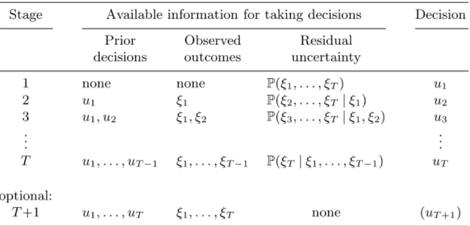
Figure 1.(From left to right) Nested partitioning of the event spaceΩ, starting from a trivial partition representing the absence of observations. (Rightmost) Scenario tree corresponding to the partitioning process.

actually realized will be gradually revealed. No branchings in the representation of the outcomes of the random process would mean that after conditioning on the observation ofξ1, the outcome ofξ2, . . . , ξT could be predicted (anticipated) exactly. Under such a representation, decisions spanning stages 2 toT would be optimized on the anticipated outcome. This would be equivalent to optimizing a nominal plan for u2, . . . , uT that fully bets on some scenario anticipated at stage 2.

To visualize how information on the realization of the random variables be-comes gradually available, it is convenient to imagine nested partitions of the event space (Figure 1): refinements of the partitions appear gradually at each decision stage in correspondence with the possible realizations of the new obser-vations. To each subregion induced by the partitioning of the event space can be associated a constant recourse decision, as if decisions were chosen according to a piecewise constant decision policy. On Figure 1, the surface of each subregion could also represent probabilities (then by convention the initial square has a unit surface and the thin space between subregions is for visual separation only). The dynamical evolution of the partitioning can be represented by a scenario tree: the nodes of the tree corresponds to the subregions of the event space, and the edges between subregions connect a parent subregion to its refined subregions obtained by one step of the recursive partitioning process.

Ideally, a scenario tree should cover the totality of possible outcomes of a ran-dom process. But unless the support of the distribution of the ranran-dom variables is finite, no scenario tree with a finite number of nodes can represent exactly the random process and the probability measure, as we already mentioned, while even if the support is finite, the number of scenarios grows exponentially with the number of stages. How to exploit finite scenario tree approximations in order to extract good decision policies for general multistage stochastic programming problems involving continuous distributions will be extensively addressed in this chapter.

2.5 The Finite Scenario-Tree Based Approximation

In the general decision model, the agent is assumed to have access to the joint probability distributions, and is able to derive from it the conditional distribu-tions listed in Table 1. In practice, computational limitadistribu-tions will restrict the quality of the representation ofP. Let us however reason at first at an abstract and ideal level to establish the program that an agent would solve for planning under uncertainty.

For brevity, let ξ denote (ξ1, . . . , ξT), and letπ(ξ) denote a decision policy mapping realizations ofξ to realizations of the decision processu1, . . . , uT. Let

πt(ξ) denote ut viewed as a function of ξ. To be consistent with the decision stages, the policy must benon-anticipative, in the sense thatutcannot depend on observations relative to subsequent stages. Equivalently one can say that π1

must be a constant-valued function, π2 a function of ξ1, and in general πt a function ofξ1, . . . , ξt−1fort= 2, . . . , T.

The planning problem can then be stated as the search for a non-anticipative policy π, restricted by the feasibility sets_Ut, that minimizes an expected total cost f spanning the decision stages and determined by the scenarioξ and the decisionsπ(ξ):

S : minimize E{f(ξ, π(ξ))_} subject to πt(ξ)∈ Ut(ξ) ∀t,

π(ξ) non-anticipative .

Here we used an abstract notation which hides the nested expectations cor-responding to the successive random variables, and the possible decomposition of the functionf among the different decision stages indexed by t. It is possible to be even more general by replacing the expectation operator by a functionalΦ assigning single numbers in R∪ {±∞} to distributions. We also stressed the possible dependence of_Utonξ1, u1, ξ2, u2, . . . , ξt−1 by writingUt(ξ).

A program more amenable to numerical optimization techniques is obtained by representingπ(_·) by a set of optimization variables for each possible argument of the function. That is, for each possible outcome ξk _{= (ξ}k

1, . . . , ξTk) ofξ, one associates the optimization variables (uk

1, . . . , ukT), written uk for brevity. The non-anticipativity of the policy can be expressed by a set of equality constraints: for the first decision stage we require uk

1 = u

j

1 for all k, j, and for subsequent

stages (t > 1) we require uk

t = u

j

t for each (k, j) such that (ξ1k, . . . , ξkt−1) ≡

(ξ1j, . . . , ξ

j t−1).

A finite-dimensional approximation to the program_S is obtained by consid-ering a finite number n of outcomes, and assigning to each outcome a discrete probabilitypk_{. This yields a formulation on a scenario tree covering the} scenar-iosξk_: S0 : minimize Pn_k=1pk_f(ξk_{, u}k₎ subject to ukt ∈ Ut(ξk) ∀k, ∀t ; uk 1 =uj1 ∀k, j ; ukt =u j t whenever (ξ1k, . . . , ξtk−1)≡(ξ1j, . . . , ξ j t−1) .

Once again we used a simple notation ξk _{for designating outcomes of the} processξ, which hides the fact that outcomes can share some elements according to the branching structure of the scenario tree.

Non-anticipativity constraints can also be accounted for implicitly. A partial path from the root (depth 0) to some node of depthtof the scenario tree identifies some outcome (ξk

1, . . . , ξkt−1) of (ξ1, . . . , ξt−1). To the node can be associated the

decision uk

t+1, but also all decisions u

j t+1 such that (ξ1k, . . . , ξtk) ≡ (ξ j 1, . . . , ξ j t). Those decisions are redundant and can be merged into a single decision on the tree, associated to the considered node of depth t (the reader may refer to the scenario tree of Figure 1).

12

The finite scenario tree approximation is needed because numerical optimiza-tion methods cannot handle directly problems like_S, which cannot be specified with a finite number of optimization variables and constraints. The approxi-mation may serve to provide an estimate of the optimal value of the original program; it may also serve to obtain an approximate first-stage decisionu1.

Sev-eral aspects regarding the exploitation of scenario-tree approximations and the derivation of decisions for the subsequent stages will be further discussed in the chapter.

Finally, we point out that there are alternative numerical methods for solving stochastic programs (usually two-stage programs), based on the incorporation of the discretization procedure into the optimization algorithm itself, for instance by updating the discretization or carrying out importance sampling within the iterations of a given optimization algorithm (Norkin, Ermoliev, & Ruszczy´nski, 1998), or by using stochastic subgradient methods (Nemirovski, Juditsky, Lan, & Shapiro, 2009). Also, heuristics for finding policies directly have been suggested: a possible idea (akin to direct policy search procedures in Markov Decision Pro-cesses) is to optimize a combination of feasible non-anticipative basis policies πj_{(ξ) specified beforehand (Koivu & Pennanen, 2010).}

2.6 Numerical Optimization of Stochastic Programs

The program formulated on the scenario tree is solved using numerical optimiza-tion techniques.

In principle, it is the size, the class and the structure of the program that determine which optimization algorithm is suitable. The size depends on the number of optimization variables and the number of constraints of the program. It is therefore influenced by the number of scenarios, the planning horizon, and the dimension of the decision vectors. The class of the program depends on the range of the optimization variables (set of permitted values), the nature of the objective function, and the nature of the equality and inequality constraints that define the feasibility sets. The structure depends on the number of stages, the nature of the coupling of decisions between stages, the way random variables intervene in the objective and the constraints, and on the joint distribution of the random variables (independence assumptions or finite support assumptions can sometimes be exploited). The structure determines whether the program can be decomposed in smaller parts, and where applicable, to which extent sparsity and factorization techniques from linear algebra can alleviate the complexity of matrix operations.

Note that the history of mathematical programming has shown a large gap between the complexity theory concerning some optimization algorithms, and the performance of these algorithms on problems with real-world data. A notable example (not directly related to stochastic programming, but striking enough to be mentioned here) is the traveling salesman problem (TSP). The TSP consists in finding a circuit of minimal cost for visitingncities connected by roads (say that costs are proportional to road lengths). The dynamic programming approach, based on a recursive formulation of the problem, has the best known complexity bound: it is possible to find an optimal solution in time proportional to n2₂n_. But in practice only small instances (n∼20) can be solved with the algorithm developed by Bellman (1962), due to the exponential growth of a list of optimal subpaths to consider. Linear programming approaches based on the simplex

algorithm have an unattractive worst-case complexity, and yet such approaches have allowed to solve large instances of the problem —n= 85900 for the record on pla85900 obtained in 2006 — as explained in Applegate, Bixby, Chv´atal, and Cook (2007).

In today’s state of computer architectures and optimization technologies, multistage stochastic programs are considered numerically tractable, in the sense that numerical solutions of acceptable accuracy can be computed in acceptable time, when the formulation is convex. The covered class includes linear programs (LP) and convex quadratic programs (QP), which are similar to linear programs but have a quadratic component in their objective. A problem can be recognized to be convex if it can be written as a convex program; a program minCF is convex if (i) the feasibility setC is convex, that is, (1−λ)x+λy∈Cwhenever x, y ∈C and 0< λ <1 (Rockafellar, 1970, page 10); (ii) the objective function F is convex onC, that is,F((1−τ)x+τ y)≤(1−τ)F(x) +τ F(y), 0< τ <1, for everyx, y∈C(Rockafellar, 1970, Theorem 4.1). We refer to Nesterov (2003) for an introduction to complexity theory for convex optimization and to interior-point methods.

Integer programs (IP) and mixed-integer programs (MIP) are similar to lin-ear programs but have integrality requirements on all (IP) or some (MIP) of their optimization variables. The research in stochastic programming for these classes is mainly focused on two-stage models: computationally-intensive meth-ods for preprocessing programs so as to accelerate the repeated evaluation of integer recourse decisions (Schultz, Stougie, & Van der Vlerk, 1998); convex re-laxations (Van der Vlerk, 2009); branch-and-cut strategies (Sen & Sherali, 2006). In large-scale applications, the modeling and numerical optimization aspects are closely integrated: see, for instance, the numerical study of Verweij, Ahmed, Kleywegt, Nemhauser, and Shapiro (2003). Solving multistage stochastic mixed-integer models is extremely challenging, but significant progress has been made recently (Escudero, 2009).

In our presentation, we focus on convex problems, and use Matlab for gen-erating the data structure and values of the scenario trees, and cvx (Grant & Boyd, 2008, 2009) for formulating and solving the resulting programs — cvx is a modeling tool: it uses a language close to the mathematical formulation of the models, leading to codes that are slower to execute but less prone to errors. 2.7 Example

To fix ideas, we illustrate the scenario tree technique on a trajectory tracking problem under uncertainty with control penalization. In the proposed example, the uncertainty is such that the exact problem can be posed on a small finite scenario tree.

Say that a random process ξ = (ξ1, ξ2, ξ3), representing perturbations at

timet= 1,2,3, has 7 possible outcomes, denoted byξk, 1≤k≤7, with known probabilitiespk_: k 1 2 3 4 5 6 7 ξk 1 -4 -4 -4 3 3 3 3 ξk 2 -3 2 2 -3 0 0 2 ξk 3 0 -2 1 0 -1 2 1 pk 0.1 0.2 0.1 0.2 0.1 0.1 0.2

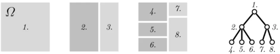
14 -4 -3 0 2 -2 1 3 -3 0 0 -1 2 2 1 0.1 0.2 0.1 0.2 0.1 0.1 0.2 b b b b b b b b b b b b b b b b b b b b b v1 v2 v3 b b b b b b b b b b b b b b b b b b b b b -0.1 2.1 -1.16 2 0.667 1.26 -0.74 -2 x1 x2 x3 x4 b b b b b b b b b b b b b b b b b b b b b b b b b b b b 0 -4.1 2.9 -5 0 -1.26 1.74 3.74 -3 -1.333 1.667 0 0 3 2.74

Figure 2.(Left) Scenario tree representing the 7 possible scenarios for a random pro-cess ξ = (ξ1, ξ2, ξ3). The outcomes ξ

k

t are written in bold, and the scenario proba-bilitiespk

are reported at the leaf nodes. (Middle) Optimal actions vt for the agent, displayed scenario per scenario, with frames around scenarios passing by a same tree node. (Right) Visited statesxtunder the optimal actions, treated as artificial decisions (see text).

The random process is fully represented by the scenario tree of Figure 2 (Left) — the first possible outcome is ξ1 _{= (}

−4,₋3,0) and has probabilityp1 _{= 0.1.}

Note that the random variablesξ1, ξ2,ξ3 are not mutually independent.

Assume that an agent can choose actionsvt∈Ratt= 1,2,3 (the notationvt instead ofutis justified in the sequel). The goal of the agent is the minimization of an expected sum of costs E{P3

t=1ct(vt, xt+1)|x1= 0}. Here xt ∈ R is the state of a continuous-state, discrete-time dynamical system, that starts from the initial state x1 = 0 and follows the state transition equation xt+1 =xt+ vt+ξt. Costsct(vt, xt+1), associated to the decisionvtand the transition to the state xt+1, are defined by ct = (dt+1+v2t/4) with dt+1 = |xt+1−αt+1| and

α2 = 2.9, α3 = 0, α4 = 0 (αt+1: nominal trajectory, chosen arbitrarily; dt+1:

tracking error;v2

t/4: penalization of control effort).

An optimal policy mapping observations ξ1, . . . , ξt−1 to decisions vt can be obtained by solving the following convex quadratic program over variables vk

t, xkt+1, dkt+1, wherekruns from 1 to 7 andt from 1 to 3, and overxk1 trivially

set to 0: minimize P7 k=1 pk P3 t=1(dkt+1+ (vkt)2/4) subject to ₋dkt+1≤xkt+1−αt+1≤dkt+1 ∀k, t xk1 = 0 , xkt+1=xkt +vtk+ξtk ∀k, t v11=v12=v31=v14=v51=v16=v17 v1 2 =v22=v32 , v24=v52=v26=v72 v32=v33 , v35=v36 .

Here, the vector of optimization variables (vk

1, xk1) plays the role of uk1, the

vector (vk

t, xkt, dkt) plays the role ofutk fort= 2,3, and the vector (xk4, dk4) plays

the role of uk

4, showing that the decision process u1, . . . , uT+1 of the general

multistage stochastic programming model can in fact include state variables and more generally any element that serves to evaluate costs conveniently.

The following code allows to formulate and solve the program using Matlab and cvx. It is almost a direct transcription of the program formulation, with variables and constraints defined in matrix form (column indices are relative to scenarios). Note that cvx replicates scalars if needed in componentwise con-straints.

% problem data xi = [-4 -4 -4 3 3 3 3;... -3 2 2 -3 0 0 2;... 0 -2 1 0 -1 2 1]; p = [.1 .2 .1 .2 .1 .1 .2]; a = [2.9 0 0]’; x1 = 0; n = 7; T = 3; % call cvx toolbox cvx_begin variables x(T+1,n) d(T,n) v(T,n) minimize( sum(sum(d*diag(p))) ... + sum(sum((v.^2)*diag(p)))/4); subject to -d <= x(2:T+1,:)-a(:,ones(1,n)); x(2:T+1,:)-a(:,ones(1,n)) <= d; x(1,:) == x1; for t=1:T x(t+1,:) == ... x(t,:)+v(t,:)+xi(t,:); end v(1,2:n) == v(1,1); v(2,2:3) == v(2,1); v(2,5:n) == v(2,4); v(3,3) == v(3,2); v(3,6) == v(3,5); cvx_end % display solution cvx_optval, v, x

The code should return the optimal objective value +7.3148. The correspond-ing optimal solution is depicted on Figure 2. In the next section, we will dis-cuss the differences between stochastic programming approaches and Markov Decision Processes. In this example, observe that the final solution can be re-cast as mappings ˜πt from xt to vt, namely, ˜π1(0) = −0.1, ˜π2(−4.1) = 2.1,

˜

π2(2.9) = −1.16, ˜π3(−5) = 2, ˜π3(−1.26) = 1.26, ˜π3(0) = 0.667, ˜π3(1.74) =

−0.74, ˜π3(3.74) =−2. Hence in this case, the convenient assumption of an agent

able to observeξtinstead of the system statextis not a fundamental restriction. Observe also that finding in this example the optimal mapping from xt to vt by a Markov Decision Process formulation is not straightforward, because the decision and state variables — to which the past states of the processξtshould be added, as the process is not memoryless — are continuous and unbounded.

3

COMPARISON TO RELATED APPROACHES

This section discusses several modeling and algorithmic complexity issues raised by the multistage stochastic programming framework and scenario-tree based decision making.

16

3.1 The Exogenous Nature of the Random Process

A frequent assumption made in the stochastic programming framework is that decision makers do not influence by their decisions the realization of the random process representing the uncertainty. The random process is said to beexogenous. This allows to simulate, select and organize in advance possible realizations of the exogenous process, before any observation is actually made, and then optimize jointly (by opposition to individually for each scenario) the decisions contingent to the possible realizations.

The need to decouple the description of uncertainties and the optimization of decisions might appear at first as a strong limitation on the situations that can be modeled and treated by stochastic programming techniques. This impression is in part justified for a large family of problems of control theory in which the uncertainty is identified to some zero-mean noise perturbing the observations or the dynamics of the system, or when the uncertainty is understood as the uncertainty on the value of system parameters However, in another large fam-ily of sequential decision making problems under uncertainty, major sources of uncertainty are precisely the ones that are the less influenced by the behavior of the decision makers (weather, interest rate evolution, accidental pollution, new regulations, for example). We also note that random processes strongly in-fluenced by the behavior of the decision makers can sometimes be handled by incorporating them to the initial decision process and treating them as a virtual decision process.

A probabilistic reasoning based on a subset of possible scenarios could easily be tricked by an adversarial random process that would exploit one of the scenar-ios discarded during the planning process. In many practical problems however, the environment is not totally adversarial. In situations where the environment is mildly adversarial, it is often possible to choose measures of performances that are more robust to bad outcomes, and that can still be optimized in a tractable way. We will come back to issues posed by risk-sensitive models for sequential decision making at the end of the chapter.

Finally, it is easier in terms of sample complexity to learn a model (find model parameters from finite data sets) for an exogenous process than for an endogenous process. Learning a model for an exogenous process is possible from observations of the process, such as time series, whereas learning a model for an endogenous process forces us to be able to simulate possible state transitions for every possible action, or at least to have at one’s disposal a fairly exhaustive data set relating actions to state transitions.

The scheduling of electric power units (Carpentier, Cohen, & Culioli, 1996; Sen, Yu, & Genc, 2006) and the management of cash flows, assets and liabilities (Dempster et al., 2008) are example of sequential decision making problems with exogenous processes following sophisticated models.

3.2 Comparison to Markov Decision Processes

In Markov Decision Processes (MDP), the decision maker seeks to optimize a performance criterion decomposed into a sum of instantaneous rewards. The information state of the decision maker at timet coincides with the state xt of a dynamical system For simplicity, we do not consider in this discussion partial observability (POMDP) or risk-sensitivity, for which the system state need not

be the information state of the agent. Optimal decision policies are often found by a reasoning based on the dynamic programming principle, to which is essential the notion of state as a sufficient statistic for representing the complete history of the system’s evolution and agent’s beliefs.

Multistage stochastic programming problems could be viewed as a subclass of finite-horizon Markov Decision Processes, by identifying the growing history of observations (ξ1, . . . , ξt−1) to the agent’s state. However, the mathematical

assumptions under the MDP and the stochastic programming formulations are in fact quite different. Complexity results suggest that the algorithmic resolution of MDPs is efficient when the decision space is finite and small (Littman, Dean, & Kaelbling, 1995; Kearns, Mansour, & Ng, 2002), while for the scenario-tree based stochastic programming framework, the resolution is efficient when the optimization problem is convex — in particular the decision space is continuous — and the number of decision stages is small (Shapiro, 2006).

One of the main appeals of stochastic programming techniques is their ability to deal efficiently with high-dimensional continuous decision spaces structured by numerous constraints, and with sophisticated, non-memoryless random pro-cesses. At the same time, if stochastic programming models have traditionally been used for optimizing long-term decisions that are implemented once and have lasting consequences, for example in network capacity planning, they are now increasingly used in the context of near-optimal control strategies that Bertsekas (2005) callslimited-lookaheadstrategies. In this usage, at each decision stage an updated model over the remaining planning horizon is rebuilt and optimized on the fly, from which only the first-stage decisions are actually implemented. In-deed, when a stochastic program is solved on a scenario tree, the initial search for a decision policy degenerates into the search for sequences of decisions relative to the scenarios covered by the tree. The first-stage decision does not depend on observations and can thus always be implemented on any new scenario, whereas the recourse decisions relative to any particular scenario in the tree could be in-feasible on a new scenario, especially if the feasibility sets depend on the random process.

3.3 The Curse of Dimensionality

Thecurse of dimensionalityis an algorithmic-complexity phenomenon by which computing optimal policies on higher dimensional input spaces requires an expo-nential growth of computational resources, leading to intractable problem formu-lations. In dynamic programming, the input space is the state space or a reduced parametrization of it. In practice the curse of dimensionality limits attempts to cover inputs to spaces embedded inRd withdat most equal to 5-10.

Approximate Dynamic Programming methods (ADP) (Bertsekas, 2005) and Reinforcement Learning approaches (RL) (Sutton & Barto, 1998) help to mit-igate the curse of dimensionality, for instance by attempting to cover only the regions of the input space that are actually reached under an optimal policy. An exploratory component may be added to the original dynamic programming solution strategy so as to discover the interesting regions of the input space by testing decisions. Those approaches work well in several cases:

– The structure of a near-optimal policy is known a priori. For example, policy search methods work well when a near-optimal policy can be described by a

18

small number of parameters. Value-function based methods work well when there is a finite and rather small set of actions, known a priori, that are the elementary building blocks of a near-optimal policy, and are used to drive the exploratory phase. Such situations are often exploited in robotics. For instance, the fundamental building blocks of near-optimal policies can be reduced to a limited number of motor primitives optimized separately. – The structure of the optimization problem is such that the promising

de-cisions and input space regions identifiable early in the exploratory phase correspond to those that are actually relevant for a near-optimal policy. This ensures the practical success of optimistic exploratory strategies, that refine decisions within regions identified as promising. This situation typi-cally arises in problems where the stochastic part comes from a noise process that slightly disturbs the dynamics of the system.

Stochastic programming algorithms do not rely on the covering of the state space of dynamic programming. Instead, they rely on the covering of the random exogenous process, which needs not correspond to the complete state space (see how the auxiliary statextis treated in the example of the previous section). The complement of the state space and the decision space are “explored” during the optimization procedure itself. The success of the approach will thus depend on the tractability of the joint optimization in those spaces, and not on insights on the structure of near-optimal policies.

In multistage stochastic programming approaches, the curse of dimensionality is present when the number of decision stages increases, and in face of high-dimensional exogenous processes. Therefore, methods that one could call, by analogy to ADP,approximate stochastic programming methods, will attempt to cover only the realizations of the exogenous random process that are truly needed to obtain near-optimal decisions. These methods work with a number of scenarios that does not grow exponentially with the dimension of the exogenous process and the number of stages.

3.4 The Value of Multistage Stochastic Programming

Due to the curse of dimensionality, multistage stochastic programming is in competition with more tractable decision models. At the same time it provides a unifying framework between several simplified decision making paradigms, that we now describe.

Reduction to Model Predictive Control. A radical simplification consists in discarding the detailed probabilistic information on the uncertainty, taking a nominal scenario, and optimizing decisions on the nominal scenario. As the common practice for defining a nominal scenario is to replace random variables by their expectation, the resulting problem on the nominal scenario is called the expected value problem, the solution of which constitutes a nominal plan. Even if the nominal plan could be used as anopen-loop decision policy, that is, implemented over the complete planning horizon, decision makers will usually want to recompute the plan at the next decision stage by solving an updated expected value problem on a new nominal scenario that incorporates the obser-vations. In the control community, the approach is known as Model Predictive

Control (MPC). We refer the reader with a background in reinforcement learn-ing to Ernst, Glavic, Capitanescu, and Wehenkel (2009) for discussions on this area of research.

An indicator of the value of multistage programming decisions over model predictive control decisions is given by thevalue of the stochastic solution(VSS). To make the notion precise, let us define successively:

– V∗

, the optimal value of the multistage stochastic program minπE{f(ξ, π(ξ))}. For notational simplicity, we adopt the convention thatf(ξ, π(ξ)) =_∞if the policyπis anticipative or yields infeasible decisions.

– ζ= (ζ1, . . . , ζT), the nominal scenario.

– uζ_{, the optimal solution to the expected value problem min}

uf(ζ, u). Note that the optimization is over a single fixed sequence of feasible decisions; the problem data is determined byζ.

– uζ1, the first-stage decision ofuζ.

– Vζ_{, the optimal value of the multistage stochastic program min}

πE{f(ξ, π(ξ))} subject to the additional constraintπ1(ξ) =uζ1for allξ. If by a slight abuse

of notation, we writeπ1, viewed as an optimization variable, for the value

of the constant-valued functionπ1, then the additional constraint is simply

π1=uζ1. By definition,Vζ is the value of a policy implementing the first

de-cision from the expected value problem, and then selecting optimal recourse decisions for the subsequent decision stages. The recourse decisions differ in general from those that would be selected by a policy optimal for the original multistage program.

The VSS is then defined as the difference Vζ

−V∗

≥ 0. For maximization problems, it would be defined by V∗

−Vζ

≥0. J. Birge and Louveaux (1997) describe special cases (with two decision stages, and restrictions on the way randomness affects problem data) for which it is possible to compute bounds on the VSS. They also come to the conclusion, from their survey of works studying the VSS, that there is no rule that can predict a priori whether the VSS is low or high for a given problem instance — for example increasing the variance of random variables may increase or decrease the VSS.

Reduction to Two-Stage Stochastic Programming. A less radical simpli-fication consists in discarding the distinction between recourse stages, keeping in the model a first stage (associated to full uncertainty) and a second stage (associated to the full knowledge of the realized scenario). A multistage model degenerates into a two-stage model when the scenario tree has branchings only at one stage (we have already described how random variables and decisions should be merged if observations and decisions are not intertwined). The situation arises for instance when scenarios are sampled over the full horizon independently: the tree has then branchings only at the root. Huang and Ahmed (2009) define the

value of multistage programming(VMS) as the difference of the optimal values of the multistage model versus the two-stage model. The authors establish bounds on the VMS and describe an application (in the semiconductor industry) where the VMS is high. Note however that a generalization of the notion of VSS would rather quantify how multistage decisions outperform two-stage decisions when those two-stage decisions are implemented with model rebuilding at each stage, in the manner of the Model Predictive Control scheme.

20

Reduction to Heuristics based on Parametric Optimization. As an in-termediate simplification between the expected value problem and the reduction to a two-stage model, it is possible to optimize sequences of decisions separately on each scenario. The decision maker can then use some averaging, consen-sus or selection strategy to implement a first-stage decision inferred from the so-obtained ensemble of first-stage decisions. Here again, the model should be rebuilt with updated scenarios at each decision stage.

The problem of computing optimal decisions separately for each scenario is known as thedistribution problem. The problem appears in the definition of the

expected value of perfect information (EVPI), which quantifies the additional value that a decision maker could reach in expectation if he or she were able to predict the future. To make the notion precise, let V∗

denote as before the optimal value of the multistage stochastic program minπE{f(ξ, π(ξ))}over non-anticipative policies π; let V(ξ) denote the optimal value of the deterministic program minuf(ξ, u); and let VA be the expected value of V(ξ), according to the distribution ofξ. Observe thatVA _{is also the optimal value of the program} minπAE{f(ξ, πA(ξ))} over anticipative policiesπA, the optimization of which

is now decomposable among scenario subproblems. The EVPI is then defined as the difference V∗

−VA

≥ 0. For maximization problems, it is defined by VA

−V∗

≥0. Intuitively, the EVPI is high when having to delay adaptations to final outcomes due to a lack of information results in high costs.

The EVPI is usually interpreted as the price a decision maker would be ready to pay to know the future (Raiffa & Schlaifer, 1961; J. R. Birge, 1992). The EVPI also indicates how valuable the dependence of decision sequences is on the particular scenario they are optimized over. Mercier and Van Hentenryck (2007) show on an example with low EVPI how a strategy based on a particular aggregation of decisions optimized separately on deterministic scenarios can be arbitrarily bad. Thus even if the EVPI is low, heuristics based on the decisions of anticipative policies can perform poorly.

This does not mean that the approach cannot perform well in practice. Van Hentenryck and Bent (2006) have studied and refined various aggregation and regret-minimization strategies on a series of stochastic combinatorial prob-lems already hard to solve on a single scenario, as well as schemes that build a bank of pre-computed reference solutions and then adapt them online to acceler-ate the optimization on new scenarios. They show that their stracceler-ategies perform well on vehicle routing applications.

Remark on the Progressive Hedging Algorithm. The progressive hedging algorithm (PHA) of Rockafellar and Wets (1991) is a decomposition method that computes the solution to a multistage stochastic program on a scenario tree by solving repeatedly separate subproblems on the scenarios covered by the tree. First-stage decisions and other decisions coupled by non-anticipativity constraints are obtained by aggregating the decisions of the concerned scenarios, in the spirit of the heuristics based on the distribution problem presented above. The algorithm modifies the scenario subproblems at each iteration to make the decisions coupled by non-anticipativity constraints converge towards a common and optimal decision.

As the iterations are carried out, first-stage decisions evolve from decisions hedged by the aggregation strategy to decisions hedged by the multiple recourse

decisions computed on the scenario tree. Therefore, the progressive hedging al-gorithm shows that there can be a smooth conceptual transition between the decision model based on the distribution problem and the decision model based on the multistage stochastic programming problem.

3.5 Example

We illustrate the computation of the VSS and the EVPI on an artificial mul-tistage problem, with numerical parameters chosen in such a way that the full multistage model is valuable. By valuable we mean that the presented simplified decision-making schemes will output first-stage decisions that are suboptimal. If those decisions were implemented, and subsequently the best possible recourse decisions were applied, the value of the objective over the full horizon would be significantly suboptimal.

Let w1, w2, w3 be mutually independent random variables uniformly

dis-tributed on _{+1,₋1_}. Letξ= (ξ1, ξ2, ξ3) be a random walk such thatξ1=w1,

ξ2 =w1+w2,ξ3 =w1+w2+w3. Let the 8 equiprobable outcomes of ξform

a scenario tree and induce non-anticipativity constraints (the tree is a binary tree of depth 3). Consider the decision process u = (u1, u2, u3) with u2 ∈ R

and ut = (ut1, ut2) ∈ R2 for t = 1,3. Then consider the multistage stochastic

program maximize 1 8 P8 k=1{[0.8uk11−0.4(uk2/2 +uk31−ξ3k)2] +uk 32ξ3k+ [1−uk11−uk12]} subject to uk11+uk12≤1 ∀k −uk 11≤uk2≤uk11 ∀k −uk1j ≤uk3j ≤uk1j ∀k andj= 1,2 C1:uk 1=u11 ∀k C2:uk 2=u k+1 2 =u k+2 2 =u k+3 2 fork= 1,5 C3:uk 3=u k+1 3 fork= 1,3,5,7 .

The non-anticipativity constraints C1, C2, C3, which are convenient to state the problem, indicate in practice the redundant optimization variables that can be eliminated.

– The optimal value of the multistage stochastic program isV∗

= 0.35 with optimal first-stage decisionu∗

1= (1,0).

– Theexpected value problem for the mean scenario ζ = (0,0,0) is obtained by setting momentarilyξk _{= ζ}

∀ k and adding the constraints C2’:uk

2 =

u1

2 ∀k and C2’:uk3 =u13 ∀k. Its optimal value is 1 with first-stage decision

uζ1= (0,0). When equality constraints are made implicit the problem can be

formulated using 5 scalar optimization variables only.

– Thetwo-stage relaxationis obtained by relaxing the constraints C2, C3. Its optimal value is 0.6361 withuk

22

– Thedistribution problemis obtained by relaxing the constraints C1, C2, C3. Its optimal value isVA _{= 0.6444. The two extreme scenarios ξ}1 _{= (1,2,3)}

andξ8 _{= (}

−1,₋2,₋3) have first-stage decisions u1

1 =u81= (0.7778,0.2222)

and value -0.0556. The 6 other scenarios haveuk

1= (0.5556,0.3578) and value

0.8778,k= 2, . . . ,7. Note that in general, (i) scenarios with the same optimal first-stage decision and values may still have different recourse decisions, and (ii) the first-stage decisions can be distinct for all scenarios.

– The EVPI is equal toVA

−V∗

= 0.2944.

– Solving the multistage stochastic program with the additional constraint C1ζ _:uk

1=uζ1∀kyields an upper bound on the optimal value of any scheme

using the first-stage decision of the expected value problem. This value is Vζ ₌

−0.2.

– The VSS is equal toV∗

−Vζ _{= 0.55.}

– Solving the multistage stochastic program with the additional constraint C1II_:uk

1 =uII1 ∀kyields an upper bound on the optimal value of any scheme

using the first-stage decision of the two-stage relaxation model. This value is VII _{= 0.2431. Thus, the value of the multistage model over a two-stage}

model, in our sense (distinct from the VMS of Huang and Ahmed (2009)), is at leastV∗

−VII_=0.1069.

To summarize, observe the collapse of the optimal value from V∗

= 0.35 to VII_{= 0.2431 (with the first-stage decision of the two-stage model) and then to}

Vζ _{=−0.2 (with the first-stage decision of the expected value model).}

We can also consider the anticipative decision sequences of the distribution problem, and check if there exists plausible strategies that could exploit the set of first-stage decisions to output a good first-stage decision (with respect to any decision-making scheme for the subsequent stages).

– Selection strategy: Solving the multistage stochastic program with a con-straint that enforces one of the first-stage decisions extracted from the dis-tribution problem yields the following results: optimal value 0.3056 ifuk

1 =

(0.7778,0.2222), optimal value 0.2167 ifuk

1 = (0.5556,0.3578). But one has

to concede that in contrast to other simplified models, for which we solve multistage programs only to measure the quality of a suboptimal first-stage decision, the selection strategy needs good estimates of the different optimal values to actually output the best decision.

– Consensus strategy: The outcome of a majority vote out of the set of the 8 first-stage decisions would be the decision (0.5556,0.3578) associated to the scenarios 2 to 7. With value 0.2167, this turns out to be the worst decision between (0.7778,0.2222) and (0.5556,0.3578).

– Averaging strategy: The mean first-stage decision of the set of 8 first-stage decisions is ¯u1= (0.6111,0.3239). Solving the multistage program withuk1=

¯

u1 for allk yields the optimal value 0.2431.

The best result is the value 0.3056 obtained by the selection strategy. Note that we are here in a situation where the multistage program and its variants could be solved exactly, that is, with a scenario tree representing the possible outcomes of the random process exactly.

4

PRACTICAL SCENARIO-TREE APPROACHES

We now focus on a practical question essential to the deployment of a multistage stochastic programming model: if a problem has to be approximately represented by a scenario tree in order to compute a decision strategy, how should a tractable and at the same time representative scenario-tree approximation be selected for a given problem?

After some background on discretization methods for two-stage stochastic programming, we pose the scenario tree building problem in an abstract way and then discuss the antagonist requirements that make its solution very challenging. Then we review the main families of methods proposed in the literature to build tractable scenario-tree approximations for a given problem, and highlight their main properties from a theoretical point of view.

Given the difficulty of determining a priori good scenario-tree approxima-tions for many problems of practical interest (a difficulty which is to some extent surprising, given the practical success of related approximation methods for two-stage stochastic programming), there is a growing consensus on the necessity of being able to test a posteriori the quality of scenario-tree based approximations on a large independent sample of new scenarios. We present in this light a stan-dard strategy based on the so-called shrinking-horizon approach — the term is used, for instance, in Balasubramanian and Grossmann (2003).

4.1 Approximation Methods in Two-stage Stochastic Programming Let_S denote a two-stage stochastic program, where the uncertainty is modeled by a random vectorξ, possibly of high-dimension, following a certain distribu-tion with either a discrete support of large cardinality, or a continuous support. Let _S0

be an approximation to _S, where ξ is approximated by a random vec-tor ξ0

that follows a distribution with a finite discrete support, the cardinality of the support being limited by the fact that to each possible realization ofξ0

is associated optimization variables for representing the corresponding recourse decisions. To obtain a good approximation, one would ideally target the problem of finding a finite discrete distribution for ξ0

(values for the support and asso-ciated probability masses) such that any first-stage decision u0

1 optimal forS

0

yields onS a minimal regret, in the sense that with optimal recourse decisions, the value on_S of the solution made of u0

1 and of optimal recourse decisions is

close to the exact optimal value of_S. By analogy to the VSS, we could also say that the distribution for ξ0

should minimize the value of the exact program_S with respect to the approximate program_S0

.

Many authors have found it more convenient to restrict the attention on the problem of finding a finite discrete distribution forξ0

such that the optimal value of_S0

is close to the optimal value of_S, and the solutionsu0

1 optimal forS

0

are close to solutions optimal for _S. For this approach to work, one might want to impose some weak form of continuity of the objective ofS with respect to solu-tions. One may also want to ensure that small perturbations of the probability measure forξhave a bounded effect on the perturbation of optimal solutionsu1.

An interesting deterministic approach (Rachev & R¨omisch, 2002) consists in analyzing the structure of optimal policies for a given problem class, the struc-ture of the objective when the optimal policy is implicitly taken into account, and inferring from it a relevant measure of distance between two distributions,