A State Space Framework for Automatic Forecasting Using Exponential Smoothing Methods.

(1)

A State Space Framework For Automatic

Forecasting

Using Exponential Smoothing Methods

Rob J. Hyndman, Anne B. Koehler,

Ralph D. Snyder and Simone Grose

Working Paper 9/2000

August 2000

DEPARTMENT OF ECONOMETRICS

AND BUSINESS STATISTICS

(2)

using exponential smoothing methods

Rob J. Hyndman1, Anne B. Koehler2, Ralph D. Snyder1, Simone Grose1 21 August 2000

Abstract: We provide a new approach to automatic business forecasting based on an extended range of exponential smoothing methods. Each method in our taxonomy of exponential smoothing methods can be shown to be equivalent to the forecasts obtained from a state space model. This allows (1) the easy calculation of the likelihood, the AIC and other model selection criteria; (2) the computation of prediction intervals for each method; and (3) random simulation from the underlying state space model. We demonstrate the methods by applying them to the data from the M-competition and the M3-competition.

Keywords: automatic forecasting, exponential smoothing, prediction intervals, state space models.

1 Introduction

In business, there is a frequent need for fully automatic forecasting that takes into account trend, seasonality and other features of the data without need for human intervention. For example, this need arises in supply chain management where forecasts of demand are required on a regular basis for very large numbers of time series so that inventory levels can be planned to provide an accept-able level of service to customers. Current methodology involves the use of highly complicated techniques such as automatic Box-Jenkins procedures (e.g., Libert, 1984) that are often poorly under-stood, or simple exponential smoothing methods (Brown, 1959) that often do not capture the range of data adequately and for which there are often no prediction intervals provided.

1_{Department of Econometrics and Business Statistics, Monash University, VIC 3800, Australia.}

2_{Department of Decision Sciences and Management Information Systems, Miami University, Oxford, OH 45056, USA.}

(3)

Although the exponential smoothing methods have been around since the 1950s, there has not been a well-developed modelling framework incorporating stochastic models, likelihood calculation, pre-diction intervals and procedures for model selection. In this paper, we aim to fill that gap by provid-ing such a framework for exponential smoothprovid-ing methods.

We note that some important steps toward this framework were established by Gardner (1985), and Ord, Koehler & Snyder (1997). Earlier work in establishing prediction intervals for exponen-tial smoothing methods appeared in Chatfield and Yar (1991), Ord, Koehler and Snyder (1997) and Koehler, Snyder and Ord (1999).

The work of Brown (1959) and Gardner (1985) has led to the use of exponential smoothing in auto-matic forecasting (e.g., Stellwagen and Goodrich, 1999). However, we develop a more general class of methods with a uniform approach to calculation of prediction intervals, maximum likelihood es-timation and the exact calculation of model selection criteria such as Akaike’s Information Criterion. Makridakis, Wheelwright and Hyndman (1998) advocate the models in the taxonomy proposed by Pegels (1969) and extended by Gardner (1985). We shall adopt the same taxonomy (with some modi-fications) as a framework for model selection for exponential smoothing methods. Each model has a trend component and a seasonal component as given in the following table.

Seasonal Component

Trend 1 2 3

Component (none) (additive) (multiplicative)

A (none) A1 A2 A3

B (additive) B1 B2 B3

C (multiplicative) C1 C2 C3

D (damped) D1 D2 D3

Cell A1 describes the simple exponential smoothing method, cell B1 describes Holt’s linear method. The additive Holt-Winters’ method is given by cell B2 and the multiplicative Holt-Winters’ method

(4)

is given by cell B3. The other cells correspond to less commonly used but analogous methods. For each of the 12 methods in the framework, we can derive an equivalent state space formulation with a single source of error following the general approach of Ord, Koehler and Snyder (1997), hereafter referred to as OKS. This enables easy calculation of the likelihood, and provides facilities to compute prediction intervals for each model. A single source of error model is preferable to a multiple source of error model because it allows the state space formulation of non-linear as well as linear cases, and allows the state equations to be expressed in a form that coincides with the error-correction form of the usual smoothing equations. To date, a state space formulation for models A1, B1, B2 and B3 has been derived (Snyder, 1985; OKS) but not for the other models in our framework. We show in Section 3 that for each of the 12 methods in the above table, there are two possible state space models corresponding to the additive error and the multiplicative error cases. These give equivalent point forecasts although different prediction intervals and different likelihoods. One of the interesting results from our framework and methodology is that we can distinguish multiplicative seasonality (or trend) in the mean from a multiplicative error term.

We propose an automatic forecasting procedure that tries each of these 24 state space models on a given time series and selects the “best” method using the AIC.

In Section2we describe a general approach to writing the point forecast equations for each of the methods, and Section3gives the state space equations for both the additive error and multiplicative error versions of each method. Estimation and model selection is discussed in Section 4 and the results are used to formulate an automatic forecasting algorithm which is outlined in Section4.2. We experiment with several variations on the algorithm by applying it to the 1001 series from the M-Competition (Makridakis, et al., 1982). The results of these experiments are summarized in Section5

and we select the best variation of the algorithm. Section 6 describes the results of applying our algorithm to the 3003 series from the M3-competition (Makridakis and Hibon, 2000) and Section7

(5)

2 Point forecast equations

Following Makridakis, Wheelwright and Hyndman (1998), we can write each of the 12 exponential smoothing methods as follows.

`t = αPt+ (1−α)Qt (1)

bt = βRt+ (φ−β)bt−1 (2)

st = γTt+ (1−γ)st−m (3)

wheremdenotes the number of seasons in a year,P,Q,R, andTvary according to which of the cells the method belongs, andα,β,γ andφare constants. Table1shows the values ofP,Q,R, andT and the formulae for computing point forecastshperiods ahead.

These equations differ slightly from the equations given in Makridakis, Wheelwright and Hyndman (1998, page 171). First, we consider the damped trend models. Second, we useQtin place of`tin

Seasonal component

Trend 1 2 3

component (none) (additive) (multiplicative)

Pt=Yt Pt=Yt−st−m Pt=Yt/st−m A Qt=`t−1 Qt=`t−1 Qt=`t−1 (none) Tt=Yt−Qt Tt=Yt/Qt φ= 1 φ= 1 φ= 1 Ft+h=`t Ft+h=`t+st+h−m Ft+h=`tst+h−m Pt=Yt Pt=Yt−st−m Pt=Yt/st−m B Qt=`t−1+bt−1 Qt=`t−1+bt−1 Qt=`t−1+bt−1 (additive) Rt=`t−`t−1 Rt=`t−`t−1 Rt=`t−`t−1 Tt=Yt−Qt Tt=Yt/Qt φ= 1 φ= 1 φ= 1 Ft+h=`t+hbt Ft+h=`t+hbt+st+h−m Ft+h= (`t+hbt)st+h−m Pt=Yt Pt=Yt−st−m Pt=Yt/st−m C Qt=`t−1bt−1 Qt=`t−1bt−1 Qt=`t−1bt−1 (multiplicative) Rt=`t/`t−1 Rt=`t/`t−1 Rt=`t/`t−1 Tt=Yt−Qt Tt=Yt/Qt φ= 1 φ= 1 φ= 1 Ft+h=`tbht Ft+h=`tbht +st+h−m Ft+h=`tbhtst+h−m Pt=Yt Pt=Yt−st−m Pt=Yt/st−m D Qt=`t−1+bt−1 Qt=`t−1+bt−1 Qt=`t−1+bt−1 (damped) Rt=`t−`t−1 Rt=`t−`t−1 Rt=`t−`t−1 Tt=Yt−Qt Tt=Yt/Qt β < φ <1 β < φ <1 β < φ <1 Ft+h=`t+ Ft+h=`t+ Ft+h= (`t+ (1 +φ+· · ·+φh−1₎_b t (1 +φ+· · ·+φh−1)bt+st+h−m (1 +φ+· · ·+φh−1)bt)st+h−m

(6)

the equations forTt. The effect of using the equations as given in Table1is that when we update the

seasonal component we use the level`t−1and growth ratebt−1 from the previous time period rather

than the newly revised level`tfrom the current time period. This alternative form of the equations is

designed to allow the models to be written in state space form (see Section3). The equations we use for B3 are not the usual Holt-Winters equations, but are equivalent to those used by OKS. It should be noted that this change makes no difference for the models with additive seasonality, but it does change the forecasts slightly for models with multiplicative seasonality.

The formulas for damped trend are appropriate when there is trend in the time series, but one be-lieves that continuing to use the final estimate for the growth rate at the end of the historical data would lead to unrealistic forecasts. Thus, the equations for damped trend do what the name in-dicates: dampen the trend as the length of the forecast horizon increases. In Table 1, one can see that the forecast forh-periods-ahead isFt+h =`t+ (1 +φ+· · ·+φh−1)bt. The trend is dampened

by a factor ofφfor each additional future time period. Our formulas for damped trend differ from those of Gardner (1985) by a factor ofφ. Gardner begins the dampening immediately for the forecast one-period-ahead and his forecast function isFt+h =`t+ (φ+φ2+· · ·+φh)bt.

Writing (1)–(3) in their error-correction form we obtain

`t = Qt+α(Pt−Qt) (4)

bt = φbt−1+β(Rt−bt−1) (5)

st = st−m+γ(Tt−st−m). (6)

The model with fixed level (constant over time) is obtained by settingα = 0, the model with fixed trend (drift) is obtained by settingβ = 0, and the model with fixed seasonal pattern is obtained by settingγ = 0. Note also that the additive trend methods are obtained by lettingφ= 1in the damped trend methods.

(7)

3 State space models

Ord, Koehler and Snyder (1997) discuss special cases of the “single source of error” state space mod-els that underlie some of the exponential smoothing methods. We expand their work to cover all the methods in the classification outlined in Section1. For each method, we obtain two models—a model with additive errors and a model with multiplicative errors. The pointwise forecasts for the two models are identical, but prediction intervals will differ.

The general OKS framework involves a state vectorxt= (`t, bt, st, st−1, . . . , st−(m−1))and state space

equations of the form

Yt = h(xt−1) +k(xt−1)εt (7)

xt = f(xt−1) +g(xt−1)εt (8)

where {εt} is a Gaussian white noise process with mean zero and variance σ2. We define et =

k(xt−1)εtandµt=h(xt−1). ThenYt=µt+et.

The model with additive errors is written asYt =µt+εtwhereµt =F(t−1)+1denotes the one-step

forecast made at timet−1. So, in this case, k(xt−1) = 1. The model with multiplicative errors is

written asYt=µt(1 +εt). Thus,k(xt−1) =µtfor this model andεt=et/µt= (Yt−µt)/µtand hence

εtis a relative error for the multiplicative model.

All the methods in Table1can be written in the form (7) and (8). The underlying equations are given in Table2. The models are not unique. Clearly, any value of k(xt−1) will lead to identical point

forecasts for Yt. For example, Koehler, Snyder and Ord (1999) and Archibald (1994) give several

models for B3 by altering the value ofk(xt−1).

The only difference between the additive error and multiplicative error models is in the observa-tion equaobserva-tion (7). The state equation (8) can be put in exactly the same form by substituting εt =

et/k(xt−1)into each state equation. For example, consider cell A1. For the additive error model

(8)

Trend Seasonal component

component 1 2 3

(none) (additive) (multiplicative)

A µt = `t−1 µt = `t−1+st−m µt = `t−1st−m (none) `t = `t−1+αεt `t = `t−1+αεt `t = `t−1+αεt/st−m st = st−m+γεt st = st−m+γεt/`t−1 µt = `t−1+bt−1 µt = `t−1+bt−1+st−m µt = (`t−1+bt−1)st−m B `t = `t−1+bt−1+αεt `t = `t−1+bt−1+αεt `t = `t−1+bt−1+αεt/st−m (additive) bt = bt−1+αβεt bt = bt−1+αβεt bt = bt−1+αβεt/st−m st = st−m+γεt st = st−m+γεt/(`t−1+bt−1) µt = `t−1bt−1 µt = `t−1bt−1+st−m µt = `t−1bt−1st−m C `t = `t−1bt−1+αεt `t = `t−1bt−1+αεt `t = `t−1bt−1+αεt/st−m (multiplicative) bt = bt−1+αβεt/`t−1 bt = bt−1+αβεt/`t−1 bt = bt−1+αβεt/(st−m`t−1) st = st−m+γεt st = st−m+γεt/(`t−1bt−1) µt = `t−1+bt−1 µt = `t−1+bt−1+st−m µt = (`t−1+bt−1)st−m D `t = `t−1+bt−1+αεt `t = `t−1+bt−1+αεt `t = `t−1+bt−1+αεt/st−m (damped) bt = φbt−1+αβεt bt = φbt−1+αβεt bt = φbt−1+αβεt/st−m st = st−m+γεt st = st−m+γεt/(`t−1+bt−1)

Table 2: State space equations for each additive error model in the classification. Multiplicative error models are obtained by replacingεtbyµtεtin the above equations.

For the multiplicative error model

εt=et/k(xt−1) =et/`t−1 and `t=`t−1(1 +αεt) =`t−1+αet.

Thus the state equations are identical in form.

Note that not all of the 24 state space models are appropriate for all data. The multiplicative error models are not well defined if there are zeros in the data. Similarly, we don’t consider the additive error models with multiplicative trend or multiplicative seasonality if any observations are zero. Further, if the data are not quarterly or monthly (and do not have some other obvious seasonal period), then we do not consider any of the seasonal methods.

(9)

4 Estimation and model selection

Let L∗(θ,X0) =nlog n X t=1 e2_t/k2(xt−1) + 2 n X t=1 log|k(xt−1)|. (9)

ThenL∗ is equal to twice the negative logarithm of the conditional likelihood function in OKS with constant terms eliminated.

The parametersθ = (α, β, γ, φ) and initial statesX0 = (`0, b0, s0, s−1, . . . , s−m+1)can be estimated

by minimizingL∗. Alternatively, estimates can be obtained by minimizing the one-step MSE, min-imizing the one-step MAPE, minmin-imizing the residual variance σ2 or via some other criterion for measuring forecast error. We shall experiment with each of these estimation approaches in Section5. We constrain the estimation by restricting the parameters to lie within the following intervals

0.1≤α≤0.9, 0.1≤β≤0.9, 0.1≤γ ≤0.9, β≤φ≤1.

Theoretically,α, β andγ can take values in(0,1). However we use a smaller range to avoid insta-bilities occurring. We also constrain the initial statesX0 so that the seasonal indices add to zero for

additive seasonality, and add tomfor multiplicative seasonality. Models are selected using Akaike’s Information Criterion:

AIC=L∗( ˆθ,Xˆ0) + 2p

wherepis the number of parameters inθandθˆandXˆ0denote the estimates ofθandX0. We select

the model that minimizes the AIC amongst all of the 24 models that are appropriate for the data. Using the AIC for model selection is preferable to other measurements of forecast error such as the MSE or MAPE as it penalizes against models containing too many parameters.

4.1 Initialization

The non-linear optimization requires some initial values. We useα =β =γ = 0.5andφ= 0.9. The initial values of`0,b0 andsk(k=−m+ 1, . . . ,0) are obtained using the following heuristic scheme.

(10)

• For seasonal data, compute a2×mMA through the first few years of data (we use up to four years if the data are available). Denote this by{ft},t=m/2 + 1, m/2 + 2, . . ..

• For additive seasonality, we detrend the data to obtainYt−ft. For multiplicative seasonality,

we detrend the data to obtainYt/ft. Then compute initial seasonal indices,s−m+1, . . . , s0, by

averaging the detrended data for each season over the first 3 years available (fromt=m/2 + 1 tot= 7m/2). We normalize these seasonal indices so they add to zero for additive seasonality, and add tomfor multiplicative seasonality.

• For seasonal data, compute a linear trend using OLS regression on the first 10 seasonally ad-justed values (using the seasonal indices obtained above) against a time variablet= 1, . . . ,10.

• For non-seasonal data, compute a linear trend on the first 10 observations against a time vari-ablet= 1, . . . ,10.

• Then set`0to be the intercept of the trend.

• For additive trend, setb0to be the slope of the trend.

• For multiplicative trend, setb0= 1 +b/awhereadenotes the intercept andbdenotes the slope

of the fitted trend.

These heuristic values of the initial stateX0are then refined by estimating them as parameters along

with the elements ofθ.

4.2 Automatic forecasting

We combine the preceding ideas to obtain a robust and widely applicable automatic forecasting al-gorithm. The steps involved are summarized below.

• We apply each of the 24 models that are appropriate to the data, and optimize the parameters of the model in each case to suit the data, starting with the initial values given in Section4.1.

• We select the best of the models according to Akaike’s Information Criterion.

• We produce forecasts using the best model (with optimized parameters).

• To obtain prediction intervals, we use a bootstrap method by simulating5000future sample paths for{Yn+1, . . . , Yn+h} and finding theα/2and1−α/2percentiles of the simulated data

at each forecasting horizon. The sample paths are generated using the normal distribution for errors (parametric bootstrap) or using the resampled errors (ordinary bootstrap).

(11)

5 Application to M-competition data

To test the algorithm, and to experiment with the various estimation approaches possible, we applied the algorithm to the 1001 series of the M-competition data (Makridakis, et al., 1982). We tested the following five estimation methods:

1 MLE: minimizingL∗; 2 MSE: Minimizing MSE; 3 MAPE: Minimizing MAPE;

4 AMSE: Minimizing (MSE1 +MSE2 +MSE3)/3where MSEk denotes the mean square of the

k-step forecast errors;

5 Sigma: Minimizing the residual varianceσ2.

For each of the 5 methods of estimation, we computed forecasts up to 18 steps ahead (the number of steps as specified in the M-competition). Then we computed the MAPEs for all forecast horizons, averaging across all 1001 series.

Table3shows the results where the MAPE is averaged across all forecast horizons. Similar results for the 504 non-seasonal series, 89 quarterly series and 406 monthly series are given in Table4. Overall, AMSE estimation seems to perform the best, closely followed by MSE estimation.

We note that the these are out-of-sample forecast accuracy measures. The results contradict the con-clusions of Armstrong and Collopy (1992) who claim that the MSE is unreliable.

We also compared the performance of the methods on how frequently prediction intervals contained the true values of the series. For each combination of methods, we computed the percentage of true values contained in the (nominally) 95% prediction intervals. We did this using both parametric intervals (PPI) based on normally distributed errors and nonparametric intervals (NPPI) based on resampling the fitted errors. The results are reported in Tables3and5. All five estimation methods underestimate the coverage probability of prediction intervals. (This is a well-known forecasting phenomenon—see Makridakis, Wheelwright and Hyndman, 1998, p.470.) Interestingly, the methods resulting in the best MAPE values seem to give the worst coverage probabilities, and vice-versa.

(12)

Estimation MAPE PPI NPPI Method AMSE 17.63 81.9% 73.2% MSE 17.73 83.4% 74.5% Sigma 18.49 83.2% 74.2% MLE 18.55 83.1% 73.5% MAPE 19.08 85.6% 77.1%

Table 3: Average MAPE from the five estimation methods using all 1001 series. PPI gives coverage of nom-inal 95% parametric prediction intervals and NPPI gives coverage of nomnom-inal 95% nonparametric prediction intervals.

Estimation Non-seasonal Quarterly Monthly

Method AMSE 23.06 16.36 13.32 MSE 23.20 17.43 13.51 Sigma 24.12 17.06 14.26 MLE 24.61 16.84 13.99 MAPE 25.64 15.23 14.34

Table 4:Average MAPE for each seasonal subset of series. Estimation Non-seasonal Quarterly Monthly

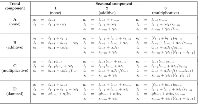
Method AMSE 79.4% 71.1% 84.7% MSE 82.0% 72.8% 85.5% Sigma 81.9% 72.2% 85.2% MLE 81.9% 72.6% 85.1% MAPE 84.1% 78.7% 87.5%

Table 5:Coverage of parametric prediction intervals for each seasonal subset of series.

Figure1shows the average MAPE for different forecast horizons separately for different subsets of the series, using the AMSE method of estimation.

For the AMSE method, we now compare our results with those obtained by other methods in the M-competition. Figure2shows the MAPE for each forecast horizon for our method and three of the best-performing methods in the M-competition. Clearly, our method is comparable in performance to these methods. Table6shows the average MAPE across various forecast horizons, and demonstrates that our method performs better than the others shown for smaller forecast horizons, but not so well for longer forecast horizons.

(13)

Figure 1:Average MAPE across different forecast horizons for all series (1001 series), non-seasonal data (504 series), quarterly data (89 series) and monthly data (406 series).

Figure 2:Average MAPE across different forecast horizons (1001 series) comparing our method with some of the best methods from the M-competition (Makridakis, et al., 1982).

(14)

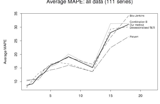
Figure 3: Average MAPE across different forecast horizons (111 series) comparing our method with some of the best methods from the M-competition (Makridakis, et al., 1982).

Forecasting horizons Average of forecasting horizons Method 1 2 3 4 5 6 8 12 15 18 1–4 1–6 1–8 1–12 1–15 1–18

Naive2 9.1 11.3 13.3 14.6 18.4 19.9 19.1 17.1 21.9 26.3 12.4 14.4 15.2 15.7 16.4 17.4

Deseasonalised SES 8.6 11.6 13.2 14.1 17.7 19.5 17.9 16.9 21.1 26.1 11.9 14.1 14.8 15.3 16.0 16.9

Combination B 8.5 11.1 12.8 13.8 17.6 19.2 18.9 18.4 23.3 30.3 11.6 13.8 14.8 15.6 16.5 17.8

Our method 9.0 10.8 12.8 13.4 17.4 19.3 19.5 17.2 23.4 29.0 11.5 13.8 14.7 15.4 16.4 17.6

Table 6: Average MAPE across different forecast horizons (1001 series).

Forecasting horizons Average of forecasting horizons Method 1 2 3 4 5 6 8 12 15 18 1–4 1–6 1–8 1–12 1–15 1–18 Naive2 8.5 11.4 13.9 15.4 16.6 17.4 17.8 14.5 31.2 30.8 12.3 13.8 14.9 14.9 16.4 17.8 Deseasonalised SES 7.8 10.8 13.1 14.5 15.7 17.2 16.5 13.6 29.3 30.1 11.6 13.2 14.1 14.0 15.3 16.8 Combination B 8.2 10.1 11.8 14.7 15.4 16.4 20.1 15.5 31.3 31.4 11.2 12.8 14.4 14.7 16.2 17.7 Box-Jenkins 10.3 10.7 11.4 14.5 16.4 17.1 18.9 16.4 26.2 34.2 11.7 13.4 14.8 15.1 16.3 18.0 Lewandowski 11.6 12.8 14.5 15.3 16.6 17.6 18.9 17.0 33.0 28.6 13.5 14.7 15.5 15.6 17.2 18.6 Parzen 10.6 10.7 10.7 13.5 14.3 14.7 16.0 13.7 22.5 26.5 11.4 12.4 13.3 13.4 14.3 15.4 Our method 8.7 9.2 11.9 13.3 16.0 16.9 19.2 15.2 28.0 31.0 10.8 12.7 14.3 14.5 15.7 17.3

(15)

A smaller set of 111 series was used in the M-competition for comparisons with some more time-consuming methods. Table 7 shows a MAPE comparison between our method and these other methods. Again, this demonstrates that our method performs better than the others shown for smaller forecast horizons, but not so well for longer forecast horizons. Figure 3 shows the MAPE for each forecast horizon for our method and the methods given in Table7. Note that our method out-performs all other methods when averaged over forecast horizons 1–4.

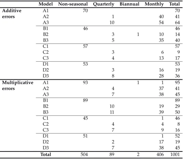
Model Non-seasonal Quarterly Biannual Monthly Total

Additive A1 70 70 errors A2 1 40 41 A3 10 54 64 B1 46 46 B2 3 1 10 14 B3 5 35 40 C1 57 57 C2 3 6 9 C3 4 13 17 D1 53 53 D2 3 16 19 D3 8 28 36 Multiplicative A1 93 1 1 95 errors A2 4 37 41 A3 7 38 45 B1 89 89 B2 10 19 29 B3 11 39 50 C1 45 1 46 C2 4 4 8 C3 7 9 16 D1 51 1 52 D2 2 17 19 D3 7 38 45 Total 504 89 2 406 1001

Table 8:Number of times each model chosen using the AIC.

Table 8 shows the models selected for each of the 1001 series using AMSE estimation. The com-monly used models A1 (simple exponential smoothing), and B1 (Holt’s method), were chosen most frequently, providing some justification for their popularity. Interestingly, the non-trended seasonal models (A2 and A3) were selected much more frequently than the popular Holt-Winters’ models (B2 and B3). Damped trend models were selected a total of 224 times compared to 268 times for

(16)

addi-tive trend, 153 times for multiplicaaddi-tive trend and 356 times for no trend. Amongst seasonal series, additive seasonality was selected 180 times, multiplicative seasonality 313 times, and no seasonal component 4 times. Of the 1001 series, an additive error model was chosen 466 times and a multi-plicative model was chosen 535 times.

For some models, the time taken for estimation of parameters was considerable (of the order of several minutes). This particularly occurred with monthly data (where there are 13 initial states to estimate) and a full trend/seasonal model (giving 4 parameters to estimate). Searching for optimal values in a space of 17 dimensions can be very time-consuming!

Consequently, we propose the following two-stage procedure to speed up the computations: 1 Estimateθwhile holdingX0at the heuristic values obtained in Section4.1.

2 Then estimateX0by minimizing AMSE while holdingθˆfixed.

This procedure speeds the algorithm by reducing the number of dimensions over which to optimize. The following table gives the average MAPE and computation time for the 1001 series from the M-competition using AMSE estimation.

Initialization MAPE Time for 1001 series Method

Heuristic only 18.14 16 min

Two-stage 17.85 22 min

Full optimization 17.63 2 hours, 20 min

The “Heuristic only” method simply uses the initial values obtained in Section 4.1, and the “Full optimization” method optimizes the initial values along with the parameters (as was done in all of the preceding computations). Clearly, very little accuracy is lost by using the two-stage method and a great deal of time can be saved.

(17)

6 Application to M3 data

Next, we applied our methodology to the M3-competition data (Makridakis and Hibon, 2000). Based on the results from the M-competition data, we used AMSE estimation and optimal initialization. The results are given in Tables9–15along with some of the methods from the M3-competition. (See Makridakis and Hibon, 2000, for details of these methods.) For each forecast horizon, we have also provided a ranking of our method compared to the 24 methods used in the M3-competition. These are based on the symmetric MAPEs averaged across series for each forecast horizon.

As with the M-competition data, our method performs best for short forecast horizons (up to 4–6 steps ahead). It seems to perform especially well on seasonal data, particularly monthly data. On the other hand, it seems to perform rather poorly on annual, non-seasonal time series.

Forecasting horizons Average of forecasting horizons Method 1 2 3 4 5 6 8 12 15 18 1–4 1–6 1–8 1–12 1–15 1–18 Naive2 10.5 11.3 13.6 15.1 15.1 15.8 14.5 16.0 19.3 20.7 12.62 13.55 13.74 14.22 14.80 15.46 B-J automatic 9.2 10.4 12.2 13.9 14.0 14.6 13.0 14.1 17.8 19.3 11.42 12.39 12.52 12.78 13.33 13.99 ForecastPRO 8.6 9.6 11.4 12.9 13.3 14.2 12.6 13.2 16.4 18.3 10.64 11.67 11.84 12.12 12.58 13.18 THETA 8.4 9.6 11.3 12.5 13.2 13.9 12.0 13.2 16.2 18.2 10.44 11.47 11.61 11.94 12.41 13.00 RBF 9.9 10.5 12.4 13.4 13.2 14.1 12.8 14.1 17.3 17.8 11.56 12.26 12.40 12.76 13.24 13.74 ForcX 8.7 9.8 11.6 13.1 13.2 13.8 12.6 13.9 17.8 18.7 10.82 11.72 11.88 12.21 12.80 13.48 Our method 8.8 9.8 12.0 13.5 13.9 14.7 13.0 14.1 17.6 18.9 11.04 12.13 12.32 12.66 13.14 13.77 Rank 4 3 7 7 12 12 8 6 7 6 4 8 6 6 6 7

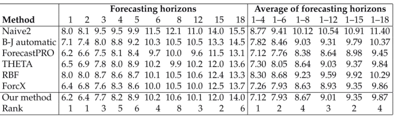
Table 9: Average symmetric MAPE across different forecast horizons: all 3003 series. Forecasting horizons Average of forecasting horizons Method 1 2 3 4 5 6 8 12 15 18 1–4 1–6 1–8 1–12 1–15 1–18 Naive2 8.0 8.1 9.5 9.5 9.9 11.5 12.1 11.0 14.0 15.5 8.77 9.41 10.12 10.54 10.91 11.40 B-J automatic 7.1 7.4 8.0 8.8 9.2 10.3 10.5 10.5 13.3 14.5 7.82 8.46 9.03 9.31 9.79 10.37 ForecastPRO 6.2 6.6 7.5 8.1 8.4 9.7 10.0 9.6 11.5 13.1 7.12 7.76 8.38 8.64 8.98 9.45 THETA 6.5 6.9 7.8 8.0 8.9 10.2 9.9 10.2 12.0 13.6 7.30 8.05 8.64 9.03 9.37 9.84 RBF 8.0 8.0 8.7 8.6 8.7 10.1 10.5 10.6 12.4 13.3 8.30 8.68 9.23 9.59 9.92 10.29 ForcX 6.4 6.8 7.6 8.3 8.6 10.0 10.5 10.0 12.5 13.7 7.26 7.93 8.63 8.93 9.35 9.86 Our method 6.2 6.4 7.7 8.2 8.9 10.2 10.6 10.1 12.0 14.0 7.12 7.93 8.67 9.01 9.35 9.87 Rank 1 1 3 5 6 4 8 3 2 6 1 2 4 3 2 4

(18)

Table 11:Average symmetric MAPE across different forecast horizons: 2141 nonseasonal series. Forecasting horizons Average of forecasting horizons

Method 1 2 3 4 5 6 1–4 1–6 Naive2 8.5 13.2 17.8 19.9 23.0 24.9 14.85 17.88 B-J automatic 8.6 13.0 17.5 20.0 22.8 24.5 14.78 17.73 ForecastPRO 8.3 12.2 16.8 19.3 22.2 24.1 14.15 17.14 THETA 8.0 12.2 16.7 19.2 21.7 23.6 14.02 16.90 RBF 8.2 12.1 16.4 18.3 20.8 22.7 13.75 16.42 ForcX 8.6 12.4 16.1 18.2 21.0 22.7 13.80 16.48 Our method 9.3 13.6 18.3 20.8 23.4 25.8 15.48 18.53 Rank 19 18 19 19 17 19 19 19

Table 12: Average symmetric MAPE across different forecast horizons: 645 annual series. Forecasting horizons Average of forecasting horizons Method 1 2 3 4 5 6 8 1–4 1–6 1–8 Naive2 5.4 7.4 8.1 9.2 10.4 12.4 13.7 7.55 8.82 9.95 B-J automatic 5.5 7.4 8.4 9.9 10.9 12.5 14.2 7.79 9.10 10.26 ForecastPRO 4.9 6.8 7.9 9.6 10.5 11.9 13.9 7.28 8.57 9.77 THETA 5.0 6.7 7.4 8.8 9.4 10.9 12.0 7.00 8.04 8.96 RBF 5.7 7.4 8.3 9.3 9.9 11.4 12.6 7.69 8.67 9.57 ForcX 4.8 6.7 7.7 9.2 10.0 11.6 13.6 7.12 8.35 9.54 Our method 5.0 6.6 7.9 9.7 10.9 12.1 14.2 7.32 8.71 9.94 Rank 4 1 7 13 17 10 20 7 9 12

(19)

Table 14:Average symmetric MAPE across different forecast horizons: 1428 monthly series. Forecasting horizons Average of forecasting horizons

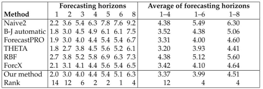
Method 1 2 3 4 5 6 8 1–4 1–6 1–8 Naive2 2.2 3.6 5.4 6.3 7.8 7.6 9.2 4.38 5.49 6.30 B-J automatic 1.8 3.0 4.5 4.9 6.1 6.1 7.5 3.52 4.38 5.06 ForecastPRO 1.9 3.0 4.0 4.4 5.4 5.4 6.7 3.31 4.00 4.60 THETA 1.8 2.7 3.8 4.5 5.6 5.2 6.1 3.20 3.93 4.41 RBF 2.7 3.8 5.2 5.8 6.9 6.3 7.3 4.38 5.12 5.60 ForcX 2.1 3.1 4.1 4.4 5.6 5.4 6.5 3.42 4.10 4.64 Our method 2.0 3.0 4.0 4.4 5.4 5.1 6.3 3.37 3.99 4.51 Rank 14 12 6 2 2 1 4 12 4 4

Table 15:Average symmetric MAPE across different forecast horizons: 174 other series.

7 Model selection accuracy

We carried out some simulations of data from the underlying stochastic state space models and then tried to identify the underlying model using the procedure outlined in Section4.2. For these sim-ulations, we used non-seasonal models and generated 5000 series for each model. The results are summarized in Table16.

The parameters used in generating these models are shown in Table 17. These parameters were chosen to generate data that look reasonably realistic.

Clearly, the algorithm has a very high success rate at determining whether the errors should be additive or multiplicative. The main source of error in model selection is mis-selecting the trend component, especially for damped trend models. That is not surprising given the value ofφchosen was very close to 1.

(20)

Additive error Multiplicative error A1 B1 C1 D1 A1 B1 C1 D1 Correct model selections 78.6 77.6 73.1 43.7 87.6 76.5 45.9 23.5 Correct additive/multiplicative selections 88.0 99.8 99.4 99.3 95.7 98.7 99.4 98.0 Correct trend selections 89.2 77.7 73.5 44.1 91.6 76.5 45.9 23.7

Table 16: Percentage of correct model selections based on 5000 randomly generated series of each type. Additive error Multiplicative error

A1 B1 C1 D1 A1 B1 C1 D1 α 0.50 0.20 0.08 0.20 0.70 0.70 0.70 0.70 β 0.10 0.10 0.10 0.03 0.03 0.03 φ 0.98 0.98 σ 0.10 1.00 0.15 1.00 0.11 0.11 0.11 0.11 `0 1.00 1.00 0.10 1.00 1.00 1.00 0.03 1.00 b0 0.20 1.05 0.20 0.10 1.04 0.10

Table 17: Parameters and initial states used in generating random data from each model.

8 Conclusions

We have introduced a state space framework that subsumes all the exponential smoothing models and which allows the computation of prediction intervals, likelihood and model selection criteria. We have also proposed an automatic forecasting strategy based on the model framework.

Application of the automatic forecasting strategy to the M-competition data and IJF-M3 competition data has demonstrated that our methodology is particularly good at short term forecasts (up to about 6 periods ahead). We note that we have not done any preprocessing of the data, identification of outliers or level shifts, or used any other strategy designed to improve the forecasts. These results are based on a simple application of the algorithm to the data. We expect that our results could be improved further if we used some sophisticated data preprocessing techniques as was done by some of the competitors in the M3 competition.

For several decades, exponential smoothing has been considered an ad hoc approach to forecasting, with no proper underlying stochastic formulation. That is no longer true. The state space framework we have described brings exponential smoothing into the same class as ARIMA models, being widely applicable and having a sound stochastic model behind the forecasts.

(21)

9 References

ARCHIBALD, B.C. (1994) “Winters Model: three versions, diagnostic checks and forecast perfor-mances”, Working paper WP-94-4, School of Business Administration, Dalhousie University, Hal-ifax, Canada.

ARMSTRONG, J.S. and F. COLLOPY (1992) Error measures for generalizing about forecasting

meth-ods: empirical comparisons,Int. J. Forecasting,8, 69–80.

BROWN, R.G. (1959)Statistical forecasting for inventory control, McGraw-Hill: New York.

CHATFIELD, C. and M. YAR (1991) Prediction intervals for multiplicative Holt-Winters,Int. J.

Fore-casting,7, 31–37.

GARDNER, E.S. (1985) Exponential smoothing: the state of the art,Journal of Forecasting,4, 1–28.

KOEHLER, A.B., R.D. SNYDERand J.K. ORD(1999) “Forecasting models and prediction intervals for

the multiplicative Holt-Winters method”, Working paper 1/99, Department of Econometrics and Business Statistics, Monash University, Australia.

LIBERT, G. (1984) The M-competition with a fully automatic Box-Jenkins procedure,J. Forecasting,3, 325–328.

MAKRIDAKIS, S., A. ANDERSEN, R. CARBONE, R. FILDES, M. HIBON, R. LEWANDOWSKI, J. NEW

-TON, E. PARZENand R. WINKLER (1982) The accuracy of extrapolation (time series) methods: results of a forecasting competition,Journal of Forecasting,1, 111–153.

MAKRIDAKIS, S., and M. HIBON(2000) The M3-competition: results, conclusions and implications Int. J. Forecasting, to appear.

MAKRIDAKIS, S., S.C. WHEELWRIGHT and R.J. HYNDMAN (1998)Forecasting: methods and

applica-tions, John Wiley & Sons: New York.

ORD, J.K., A.B. KOEHLERand R.D. SNYDER(1997) Estimation and prediction for a class of dynamic

nonlinear statistical models,J. Amer. Statist. Assoc.,92, 1621–1629.

PEGELS, C.C. (1969) Exponential forecasting: some new variations,Management Science,12, 311–315. SNYDER, R.D. (1985) Recursive estimation of dynamic linear statistical models,J. Roy. Statist. Soc., B

47, 272–276.

STELLWAGEN, E.A., and R.L. GOODRICH(1991)Forecast Pro 4.0 manual, Business Forecast Systems: