Detecting patterns in Time Series Data with applications in Official Statistics

(1)

Detecting patterns in Time Series Data with

applications in Official Statistics

Ben Norwood, MSci (Hons.)

Department of Mathematics and Statistics Lancaster University

This thesis is submitted in partial fulfilment of the requirements for the degree of Doctor of Philosophy

(2)

Abstract

This thesis examines the issue of detecting components or features within time series data in automatic procedures. We begin by introducing the concept of Wavelets and briefly show their usage as a tool for detection. This leads to our first contribution which is a novel method using wavelets for identifying correla-tion structures in time series data which are often ambiguous with very different contexts. Using the properties of the wavelet transform we show the ability to distinguish between short memory models with changepoints and long memory models. The next two Chapters consider seasonality within data, which is often present in time series used in Offical Statistics. We first describe the historical evo-lution of identification of seasonality, comparing and contrasting methodology as it has expanded throughout time. Following this, motivated by the increased use of high-frequency time series in Official Statistics and a lack of methods for identi-fying low-frequency seasonal components within high-frequency data, we present a method for identifying periodicity in a series with the use of a simple wavelet decomposition. Presented with theoretical results and simulations, we show how the seasonality of a series is uniquely represented within a wavelet transform and use this to identify low frequency components which are often overlooked in favour of a trend, with very different interpretations. Finally, beginning with the moti-vation of forecasting European Area GDP at the current time point, we show the effectiveness of an algorithm which detects the most useful data and structures for a Dynamic Factor Model. We show its effectiveness in reducing forecasting errors but show that under large scale simulation that the recovery of the true structure

(3)

over two dimensions is a difficult task. All the chapters of this thesis are motivated by, and give applications to, time series from different areas of Official Statistics.

(4)

Acknowledgements

I’d like to take this oppurtunity to mention and thank everyone who has made this happen. Firstly I would like to thank my colleagues and friends Laura Barlow, Callum Vyner and Jessica Welding, for always providing an interesting workplace and keeping me grounded. You have all taught me so much. Thank you also to my friends who have continually waited for me to finish this: Jon, Ben and Jake, you have stuck by me whilst my head has been firmly in this thesis and I can’t acknowledge that enough. To my parents who have continually pushed me to higher levels, I would not have made it without you or your love. A very special thank you to my supervisor, and now dear friend, Dr. Rebecca Killick whom without her expertise, patience and kindness this would not have been possible.

Financial support for this work was granted by the Economic and Social Re-search Council, and for that I gratefully acknowledge them. My industrial super-visor, Duncan Elliott, and his team at The Office of National Statistics have made my time working with them invaluable.

Finally, I’d like to thank my partner Anna France. Your love and support has kept me going in ways I cannot find the words to explain. You challenge me to become better and you’ve always kept me level-headed. I consider myself very lucky that we could complete our work together.

(5)

Declaration

I declare that this thesis is my own work, and has not been submitted by myself in substantially the same form for the award of a higher degree elsewhere.

(6)

Published Work

This thesis includes the following published work

• Norwood, B., Killick, R. (2018) Long Memory and Changepoint Models: A Spectral Classification Procedure. Statistics and Computing 28(2) 291–302

• Norwood, B., Killick, R. (2016) Evolution of Seasonal Adjustment Methods. EuroStat Report, ESTAT/11111.2013.001-2013.254

• Norwood, B., Killick, R. (2019) Nowcasting: Practical Results with Theoret-ical Flaws. EuroStat Report, ESTAT/11111.2013.001-2013.254

Each piece of this work is given as Chapters 3, 4 and 6. Chapters 4 and 6 were created for Eurostat under contract number ESTAT/11111.2013.001-2013.254 through a subcontract between Lancaster University and Sogeti.

Motivations and appropriate literature reviews are provided in each of the chapters. Notation, where possible, has been kept consistent throughout and is introduced separately in each chapter. Therefore they may be read individually or as a whole. Relevant appendices are given at the end of each chapter. The bibliography for all chapters is given at the end.

(7)

5 Wavelet Frequency Detection 104 5.1 Introduction . . . 104 5.2 Methodology . . . 109 5.2.1 Wavelet Tranforms . . . 109 5.2.2 Transforms of periodicity . . . 110 5.2.3 Variance Profiles . . . 111 5.2.4 Test statistic . . . 114 5.2.5 Algorithm . . . 115 5.3 Empirical Analysis . . . 118 5.3.1 Test Power . . . 118 5.3.2 Detection Rates . . . 120 5.3.3 Estimation of p . . . 123

5.4 Application: Live Births in Metropolitan France . . . 125

(9)

5.6 Appendix . . . 130 5.6.1 Proof of Theorem 1 . . . 130 5.6.2 Proof of Theorem 2 . . . 146 5.6.3 Proof of Theorem 3 . . . 158 5.6.4 Detection Graphs n= 512,1024 . . . 159 5.6.5 Estimation Graphs n = 512,1024 . . . 160

6 Automatic Dynamic Factor Model 161 6.1 Introduction . . . 161

6.2 European Area GDP . . . 163

6.2.1 Data . . . 163

6.2.2 Previous Models . . . 166

6.3 Dynamic Factor Models . . . 166

6.3.1 Overview . . . 167

6.3.2 Structural Considerations . . . 170

6.3.3 Methodology For EAGDP . . . 172

6.3.4 Results of Application . . . 174

6.3.5 Discussion of Application . . . 179

6.4 Structural Recovery Simulations . . . 180

6.4.1 Results of Simulations . . . 182

6.4.2 Discussion of Simulations . . . 186

6.5 Generalised Algorithm Approach . . . 186

6.5.1 Exploration of Models . . . 187 6.5.2 Scoring Functions . . . 188 6.5.3 Results of Simulations . . . 190 6.5.4 Discussion of Results . . . 204 6.6 Conclusion . . . 206 6.7 Appendix . . . 208

(10)

7 Conclusion 218

(11)

List of Figures

2.1 Example Haar Wavelets upon White Noise . . . 22

2.2 Wavelet transform of a changing function . . . 26

2.3 Non-decimated wavelet transform of a changing function . . . 28

3.1 Average empiricial periodograms and wavelet spectra . . . 38

3.2 Applications of Classifier . . . 51

3.3 Inflation Diagnostics . . . 53

3.4 Stock correlation diagnostics . . . 53

5.1 French Births Data . . . 105

5.2 Average wavelet spectra of noisy sinusoid . . . 111

5.3 Scale variance of sinusoid . . . 112

5.4 Variance profiles . . . 113

5.5 Fourier Spectra and Variance Profile comparison . . . 114

5.6 Variance profiles for Gaussian White Noise . . . 115

5.7 Scale cross over points . . . 117

5.8 Results - Detection of Periodicity (n = 128,256) . . . 121

5.9 Results - Difference from Truth (n= 128,256) . . . 124

5.10 French Births Data studied . . . 126

5.11 Results of Application . . . 128

5.12 Results - Detection of Periodicity (n = 512,1024) . . . 159

5.13 Results - Difference from Truth (n= 512,1024) . . . 160

(12)

6.2 EAGDP - Structure Selected . . . 179 6.3 Dependent Model 3 Example Data . . . 182 6.4 Dependent Model 4 Example Data . . . 183

(13)

List of Tables

3.1 Classification Results - Changepoint . . . 46

3.2 Classification Results - Long Memory . . . 47

3.3 Classifier application results . . . 52

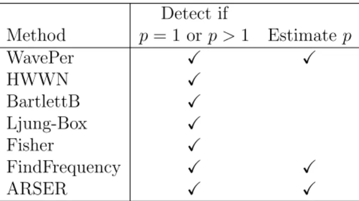
5.1 Methodology compared against . . . 118

5.2 Gaussian White Noise Results . . . 122

5.3 French Daily Births Application . . . 127

6.1 EAGDP - Data Sources . . . 165

6.2 EAGDP - Variable Inclusion Rates . . . 178

6.3 Calendar Alignment . . . 178

6.4 Independent Series . . . 181

6.5 Initial Algorithm - Simulation Results - Correct selection of structure184 6.6 Initial Algorithm - Component Selection Results . . . 185

6.7 Extended Algorithm - Initial Model Selection . . . 188

6.8 Extended Algorithm - Non-initial models . . . 189

6.9 Extended Algorithm - Simulation Results - Selection of independent series (n∗ = 24) . . . 193

6.10 Extended Algorithm - Simulation Results - Selection of dependent series (n∗ = 24) . . . 194

6.11 Extended Algorithm - Simulation Results - Selection of true amount of factors (n∗ = 24) . . . 196 6.12 Extended Algorithm - Simulation Results - Truth fitted (n∗ = 24) . 197

(14)

6.13 Extended Algorithm - Simulation Results - Consideration of Truth (n∗ = 24) . . . 199 6.14 Extended Algorithm - Simulation Results - MSE over recent 24

points (n∗ = 24) . . . 200 6.15 Extended Algorithm - Simulation Results - MSE over all points

(n∗ = 24) . . . 202 6.16 Extended Algorithm - Simulation Results - Dependent Model

Struc-ture 4 (n∗ = 24) . . . 203 6.17 Extended Algorithm - Simulation Results Overview (n∗ = 24) . . . 205 6.18 Extended Algorithm - Simulation Results - Truth fitted (n∗ = 500) 209 6.19 Extended Algorithm - Simulation Results - Selection of independent

series (n∗ = 500) . . . 210 6.20 Extended Algorithm - Simulation Results - Selection of dependent

series (n∗ = 500) . . . 211 6.21 Extended Algorithm - Simulation Results - Selection of true amount

of factors (n∗ = 500) . . . 212 6.22 Extended Algorithm - Simulation Results - Consideration of Truth

(n∗ = 500) . . . 213 6.23 Extended Algorithm - Simulation Results - MSE over recent 24

points (n∗ = 500) . . . 214 6.24 Extended Algorithm - Simulation Results - MSE over all points

(n∗ = 500) . . . 215 6.25 Extended Algorithm - Simulation Results - Dependent Model

Struc-ture 4 (n∗ = 500) . . . 216 6.26 Extended Algorithm - Simulation Results Overview (n∗ = 500) . . . 217

(15)

Chapter 1 Introduction

As technology has evolved, so has the data which we collect. Whilst accuracy and length of data is often the issue for most pracitioners, a new emerging area is the breadth, or width, of the data we collect. As the ability to store data efficiently has increased and is no longer a limiting factor to the decision maker, data is now collected from a wide variety of sources. The issue of automatically analysing and utilising data becomes ever more important when it is predicted that the total amount of new data generated in 2025 will be over five times more than that generated in 2018 (Reinsel et al., 2019) and thus we must develop methodology to meet this sudden rise in supply.

Wavelets have been used as a tool to efficiently store important features of a data set. They have grown in their popularity as a tool to succinctly decompose a series, and this thesis develops methods that continue in this vein. We begin by reviewing the key concepts and techniques used such as Wavelet Decomposition within Chapter 2. Here we present the key advantages of a time varying decom-position, and show how they have been used in other areas of statistics such as denoising and compression. Following this, in Chapter 3 we apply these particular advantages to the case of classification between ambiguous models with very differ-ent interpretations. Distinguishing between Long Memory or Short Memory with Changepoints can significantly change interpretation, and we present a solution to this ambiguity alongside applications to Price Inflation and Stock Correlation

(16)

Data.

To meet this high demand on knowledge we develop methodology for the use of data which is collected more often, or at a higher frequency. However with this comes additional concerns over interpretation, particularly in the area of seasonal adjustment. Chapter 4 reviews the methodology currently available for seasonal adjustment, providing one page overviews of the methods as they have developed through time. We then look to use the advantages of Wavelets in Chapter 5 to aid in the discovery of low frequency seasonal components which may often be overlooked as trends. We provide theoretical results for a particular type of seasonality, or periodicity and present methodology to detect and identify this component, before applying it French National Birth data.

With this increasing data availability, expectations are also rising as to the lead time of publication of information. In the domain of Official Statistics, this raises an interesting issue where data collection can only occur within a certain timeframe, but the output still needs to be estimated to meet the growing demand for timely information. Therefore methodology, colloquially referred to as ‘Now-casting’, was created for the purpose of estimating large complex systems at the current timepoint using their relationships with other more readily available data. With the motivation of European Area Gross Domestic Product, Chapter 6 looks at how these relationships change over time and how this may aid estimation of the system. With encouraging results we then extend our methodology further and test its capability to recover the truth under simulation.

(17)

Chapter 2 Wavelet Literature Review

The following chapter introduces the concept of wavelets and explains their com-mon use cases. We begin by introducing them in terms of a Multi-Resolution Analysis, before showing their relationships in the Fourier Domain. Following this we give the example of the Haar Wavelet, then show how a wavelet decompo-sition is constructed. We then explore this further by reviewing the decimated and non-decimated approaches. Continuing, we then explain the concept of Lo-cally Stationary Wavelet Processes before giving a brief review of the literature of wavelet usage. Finally we conclude by mentioning a number of other wavelet methods which we do not cover here.

2.1 Introduction

Defined seminally in Daubechies (1992) wavelets, or ‘little waves’, are a specially constructed localised function which are used to capture information and features on a local and global scale of a function or data. We begin first by formalising this concept of multi-resolution analysis, before showing the relevance of wavelet functions in this context.

Definition 2.1. A multi-resolution analysis is a collection of closed subspaces of

(18)

1. A containment hierarchy exists as such:

· · · ⊂Vj+2 ⊂Vj+1 ⊂Vj ⊂Vj−1 ⊂Vj−2 ⊂. . . (2.1)

2. There is a trivial intersection and dense union of these spaces,

\ j Vj ={0}, [ j Vj =L2(R).

3. There is a self-similarity in the spaces by scale,

f(2−jx)∈Vj ⇐⇒ f(x)∈V0.

4. Each space is invariant to translation,

f(x)∈Vj ⇐⇒ f(x+ 2−jk)∈Vj, ∀k∈Z.

5. There exists a function φ(x)∈_L2(_R), termed the scaling function, such that for all j ∈_Z and k ∈_Z; the functions 2−2jφ(2−jx+k) form an orthonormal basis for Vj.

Here and going forward, we refer to the parametersj and k as scale and trans-late respectively. It should be noted that in other literature often the index of the subspaces is negatively reversed, however we proceed as this is more natural for the algorithm development in the works that follow, as noted in Vidakovic (2009). If we now consider the scaling function, usually referred to as the father wavelet

φ(x) ∈ V0, and the hierarchy shown in Equation (2.1) we can then determine a

relationship between scaling functions. This is such that

φj+1(x) = ∞ X k=−∞ hk2− j 2φ(2−jx+k) = X k∈Z hkφj,k(x) (2.2)

(19)

additional constanthk wherek ∈Z. It is the set ofhk which form a wavelet filter,

of which we are particularly interested in. Each of these wavelet filters satisfy two main conditions: firstly normalization such thatP

k∈Zhk = √ 2; and orthogonality such that X k∈Z hkhk−2l=δl, for l ∈Z.

Consider next that following Equation (2.1) there exists a difference space between each subspace, such that

Wj =Vj−1 Vj. (2.3)

Given that we are able to determine a wavelet filterhk on a scaling function φ(x),

this implies there exists a non-unique orthonormal basis in_L2(_R) for the different spaceWj. We denote this basis by the set

{ψj,k(x) = 2 −j

2 ψ(2−jx+k) :j, k ∈Z}. (2.4)

The functionψ0,0(x) or ψ(x) is referred to as the wavelet function, or colloquially

the mother wavelet. As ψ(x)∈ W0 ⊂ V−1 we can relate the mother to the father

wavelet as ψ(x) = ∞ X k=−∞ gk 1 √ 2φ( 1 2x+k) or more generally ψj,k(x) = ∞ X k=−∞ gk2− j 2φ(2−j−1x+k).

2.2 Fourier Analysis

It is of interest to look at the properties of the mother and father wavelet in the time-frequency dimensions. Such an analysis can be done by reviewing the functions under a Fourier transformation.

(20)

given by ˆ f(ω) = F[f(x)] = Z R f(x)e−iωxdx. (2.5)

This transformation can be reversed also:

f(x) =F−1_{[ ˆ}_f₍_ω_{)] =} 1

2π

Z

ˆ

f(ω)eiωxdω.

The Fourier transformation of a function allows analysis over frequency, but sacrifices the information from the time dimension of the original function. There are many properties attached to this transformation, which we will make use of in the definitions and explanations to follow, however we do not detail them here but refer the reader to Vidakovic (2009). It can be shown that by using the properties associated with the Fourier transform, that there is a likewise recurrence relation on the scaling function. This is such that

Φ(ω) =F[φ(x)] = 2−12 X k∈Z hkexp−ikωΦ ω 2 =m0 ω 2 Φω 2 = ∞ Y j=1 Φω 2j .

Similarly we can show how the set of translates {φ(x+k)}k∈Z using the Fourier

transform as

∞

X

k=−∞

|Φ(ω+ 2πk)|2,

or similarly (but not equivalently)

|m0(ω)|2+|mo(ω+π)|2 = 1.

For more information on the difference between these two statements, please con-sult Vidakovic (2009).

Moving next to the wavelet filter, we have already shown a relationship between both functions, but we further investigate it within the Fourier domain. Following

(21)

similar calculations to those performed on the scaling function, we find that Ψ(ω) =F[ψ(x)] = 2−12 X k∈Z gkexp−ikωΨ ω 2 =m1 ω 2 Ψω 2 = ∞ Y j=1 Ψω 2j .

Most importantly, it can be shown that there exists a direct relationship between

m0 and m1:

|m0(ω)|2+|m1(ω)|2 = 1.

With these relationships we are now able to directly compute the wavelet filter coefficientsgk from hk:

gk = (−1)kh1−k. (2.6)

Known as the quadrature mirror relation, this allows us to calculate a high-pass filter (containing detail) from a low-pass (averaging) filter.

2.3 Haar Wavelet

An often used example of a wavelet is the Haar Wavelet. First discovered by Alfred Haar (Haar, 1910), its simple nature and intuitive construction aid often in the explanation of wavelets.

The scaling function for the Haar Wavelet is a simple step function of the form

φ(x) =        1 if 0≤x <1, 0 elsewhere.

It can be verified quickly that the set of functions {φ(x +k)}k∈Z forms an

or-thonormal basis forV0, as the function is non-overlapping due to the non-inclusive

upper bound on the domain, and also R_Rφ(x)dx = 1. Following Equation (2.2) withj =−1 we determine that the only relevant values of k are k =−1,0 giving,

φ(x) =h02

1

2φ(2x) +h₁2

1

(22)

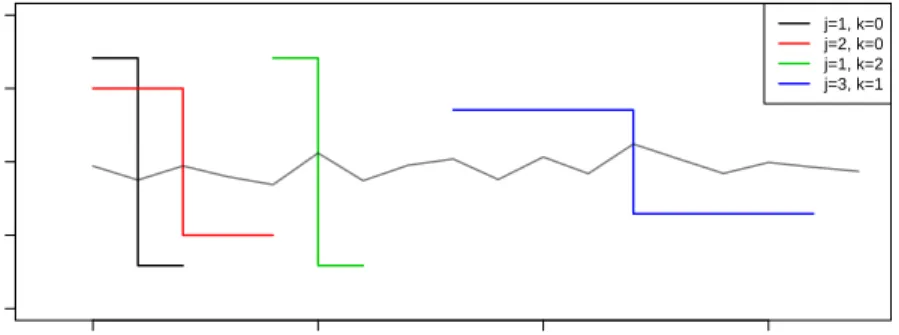
0 5 10 15 −1.0 −0.5 0.0 0.5 1.0 x ψjk j=1, k=0 j=2, k=0 j=1, k=2 j=3, k=1

Figure 2.1: A number of Haar Wavelets over different scales j and position k

superposed upon a small white noise series (N(0,0.12)) for clarity. Note that values of zero for the wavelets are not shown.

Given that we have already determined that integer translates of the haar scaling functions are non-overlapping, we can determine that h0 = h1 = √1

2. Following

on now, using the quadrature mirror filter relationship given in Equation (2.6) we can now determine that the mother waveletψ has the following form

ψ(x) =                1 if 0≤t < 1₂, −1 if 1₂ ≤t <1, 0 else,

such that there is a set of wavelet coefficients gk = {√1₂,−√1₂}. We can now

translate and scale this function as per the set definition given in Equation (2.4). An example of a number of wavelets drawn up is given in Figure 2.1.

2.4 Wavelet Decomposition

As we are now able to construct wavelet filters sufficiently, given an appropriate scaling function, we now look at a transformation to decompose a function using the orthonormal wavelet bases. First we define the coefficients generated by the

(23)

inner product of the wavelet filter and scaling function as cj,k =< f(x), φj,k(x)> = Z ∞ −∞ f(x)φj,k(x)dx, dj,k =< f(x), ψj,k(x)> = Z ∞ −∞ f(x)ψj,k(x)dx.

Then, working from the scaling equation defined earlier in Equation (2.2), we are able to create an approximation to a functionf(x) at scale j:

ˆ

fj(x) = X

k∈Z

cj,kφj,k(x),

which can be combined with the properties of the MRA given in Equation (2.1) and (2.3) to extend the approximation. This leads to

ˆ fj(x) = ˆfj−1(x) + X k∈Z dj,kψj,k(x) =X k∈Z cj,kφj,k(x) + X k∈Z dj,kψj,k(x) =X k∈Z cj0,kφj0,k(x) + j X i=j0 X k∈Z di,kψi,k(x), j0 ≤j.

This is such that we can approximate a function at scale j by the information provided at a coarser level j0 and the detail in between. If we then take an

increasing amount of scales, such thatj → ∞ we converge upon

f(x) =X k∈Z cj0,kφj0,k(x) + ∞ X i=j0 X k∈Z di,kψi,k(x).

This has a direct discrete counterpart, such that we can decompose a seriesy=

{y0, y1, . . . , yn−1} of dyadic length (∃J ∈ N : n = 2J) into ‘smooth’ components

and a number of ‘detail’ components:

(24)

2.5 Decimated Wavelet Decomposition

A direct calculation can be made for each of these components, however this can be very costly computationally. If however the scaling function satisfies the prop-erties of an MRA, then we can use the pyramidal algorithm detailed in Mallat (1989). This algorithm uses the relations between each scale to calculate the dis-crete wavelet transform of a series with order O(n) computations. To see this, consider again the scaling relationships given in Equation (2.2) and see that we can rewrite the calculation of the ‘smooth’ coefficient

cj,k = Z ∞ −∞ f(x)φj,k(x)dx= X i∈Z hicj−1,i+2k = X i∈Z hi−2kcj−1,i,

such that it relies upon the previous scale and a translation of the originalhk filter.

This applies similarly to the wavelet function,

dj,k = X

i∈Z

gi−2kcj−1,i.

Note that there are half as many coefficients that can be computed at scale

j than scale j−1. This is a consequence of the decimation that occurs between scales which is described further within Mallat (1989). Here we briefly overview it following similar notation.

Definition 2.3. Given a seriesy={. . . , y−1, y0, y1, y2, . . .}, define the application

of filters H and G as (Hy)k= X i∈Z hi−kyi, (Gy)k= X i∈Z gi−kyi.

Definition 2.4. Define the selection of each even element of a series as the binary

decimation operator D0 such that (D0y)j =y2j.

If we now let the coarest information of the transform be the original series, such that c0 = y, then we can describe the successive operations required to compute

(25)

the full transform by

cj =D0Hcj−1, dj =D0Gcj−1.

An example of this, using the Haar Wavelet given in Section 2.3 is shown in Figure 2.2, applied to the sawtooth function

f(x) =                4x2+ 4₃x if 0≤x≤ 1 3 12 8 x 2₊4 8x if 1 3 < x≤ 2 3 x2 +4₈x− 1 2 if 2 3 < x≤1 . (2.7)

2.6 Non-Decimated Wavelet Decomposition

Whilst computationally efficient, the decimated wavelet decomposition has a main disadvantage that can be seen by merely shifting the data by a single point, as shown in Figure 2.2. In particular note the shift in magnitude at the lowest scales at half the length of the series. Due to the decimation process D0, shifting the

series by a single point creates a complete new set of coefficients. This is known as the translation invariance property of the decimated wavelet transform.

To define the non-decimated transform, we must describe how to transform the filtering operations and decimation process.

Definition 2.5. Let the inverse of the binary decimation operator be such that

upon application to a series y = {. . . , y−1, y0, y1, . . .}, it adds zeros between each

element. This is such that

D−1

0 y = ˜y, where y˜={. . . ,0, y−1,0, y0,0, y1,0, . . .}.

(26)

0 10 20 30 40 50 60 0.0 0.2 0.4 0.6 0.8 1.0 Translate c0

(a) Original series.

0 10 20 30 40 50 60 Translate Scale 1 2 3 4 5 6 x x x x x x x x x x x x x x x x x x x x x x x x x x x x x x x o o o o o o o o o o o o o o o o o o o o ooo o o o o o o o o x x x x x x x x x x x x x x x x o o o o o o o o o o o o o o o o x x x x x x x x o o o o o o o o x x x x o o o o x x o o x o x o c d

(b) c and dcoefficients for each scale.

0 10 20 30 40 50 60 0.0 0.2 0.4 0.6 0.8 1.0 Translate c0

(c) Original series shifted by one point.

0 10 20 30 40 50 60 Translate Scale 1 2 3 4 5 6 x x x x x x x x x x x x x x x x x x x x x x x x x x x x x x x o o o o o o o o o ooo o o o o o o o o o o o o o o o o o o o x x x x x x x x x x x x x x x x o o o o o o o o o o o o o o o o x x x x x x x x o o o o o o o o x x x x o o o o x x o o x o x o c d

(d) c and dcoefficients for each scale. Figure 2.2: Wavelet transform of a sawtooth function. Note in Figures 2.2b and 2.2d that each coefficient has been scaled by the maximum value and is centered on a zero line, bounded above and below by 1 and -1 respectively shown by the dotted lines.

(27)

filters which are recursively related such that

H[0] ₌_H_, _H[j]₌_D−1

0 H [j−1]_,

G[0] =G, G[j]=D−₀1G[j−1].

Then the non-decimated smooth and detail coefficients sets,c¯j andd¯j are computed by

¯

cj =H[j−1]c¯j−1, d¯j =G[j−1]c¯j−1.

This then creates an overcomplete transform which considers both even and odd decimations. As such, each coefficient set is of length 2J_{. In contrary to the}

decimated wavelet transform, this is translation invariant, and often referred to as the stationary wavelet transform. Our original example given by Equation (2.7), is presented under a non-decimated wavelet transform, with a shifted version for comparison, in Figure 2.3.

2.7 Locally Stationary Wavelet Processes

We must first define a time series, before defining Locally Stationary Wavelet Processes. A time series is formally defined as a collection of data over time, such that we have a seriesytfort= 1,2, . . . , n. A common assumption in the modelling

of a time series is that it is stationary, such that its properties do not vary over time. This is often not valid, but a similar assumption of local stationarity, such that a segment of data is stationary, may often prove more useful. For a review of such processes and an overview of the literature surrounding them, Dahlhaus (2012) is recommended.

Wavelets, with their ability to localise particular characteristics across different scales and translations, provide a framework to model locally stationary wavelet processes, introduced in Nason et al. (2000).

(28)

0 10 20 30 40 50 60 0.0 0.2 0.4 0.6 0.8 1.0 Translate c0

(a) Original series.

0 10 20 30 40 50 60 Translate Scale 1 2 3 4 5 6 xxxxxxxxxxxxxxxxxxxxxxxxxxxxxxxxxxxxxxxxxxxxxxxxxxxxxxxxxxxxxxxx oooooooooooooooooooooooooooooooooooooooooooooooooooooooooooooooo xxxxxxxxxxxxxxxxxxxxxxxxxxxxxxxxxxxxxxxxxxxxxxxxxxxxxxxxxxxxxxxx oooooooooooooooooooooooooooooooooooooooooooooooooooooooooooooooo xxxxxxxxxxxxxxxxxxxxxxxxxxxxxxxxxxxxxxxxxxxxxxxxxxxxxxxxxxxxxxxx

oooooooooooooooooooooooooooooooooooooooooooooooooooooooooooooooo

xxxxxxxxxxxxxxxxxxxxxxxxxxxxxxxxxxxxxxxxxxxxxxxxxxxxxxxxxxxxxxxx

oooooooooooooooooooooooooooooooooooooooooooooooooooooo oooooo_ooo

o

oooooooooooooooooooooooooooooooooooooooooooo oooooooooo oooooooooo xxxxxxxxxxxxxxxxxxxxxxxxxxxxxxxxxxxxxxxxxxxxxxxxxxxxxxxxxxxxxxxx oooooooo oooooooooooooooooooooooooooooooo oooooooooooooooooooooooo x o c d

(b) c and dcoefficients for each scale.

0 10 20 30 40 50 60 0.0 0.2 0.4 0.6 0.8 1.0 Translate c0

(c) Original series shifted by one point.

0 10 20 30 40 50 60 Translate Scale 1 2 3 4 5 6 xxxxxxxxxxxxxxxxxxxxxxxxxxxxxxxxxxxxxxxxxxxxxxxxxxxxxxxxxxxxxxxx oooooooooooooooooooooooooooooooooooooooooooooooooooooooooooooooo xxxxxxxxxxxxxxxxxxxxxxxxxxxxxxxxxxxxxxxxxxxxxxxxxxxxxxxxxxxxxxxx oooooooooooooooooooooooooooooooooooooooooooooooooooooooooooooooo xxxxxxxxxxxxxxxxxxxxxxxxxxxxxxxxxxxxxxxxxxxxxxxxxxxxxxxxxxxxxxxx

oooooooooooooooooooooooooooooooooooooooooooooooooooooooooooooooo

ooooooooooooooooooooooooooooooooooooooooooooooooooooo oooooo_ooo

oo

ooooooooooooooooooooooooooooooooooooooooooo oooooooooo ooooooooooo xxxxxxxxxxxxxxxxxxxxxxxxxxxxxxxxxxxxxxxxxxxxxxxxxxxxxxxxxxxxxxxx oooooooo ooooooooooooooooooooooooooooooo ooooooooooooooooooooooooo x o c d

(d) c and dcoefficients for each scale. Figure 2.3: Non-decimated wavelet transform of a sawtooth function. Note in Figures 2.3b and 2.3d that each coefficient has been scaled by the maximum value and is centered on a zero line, bounded above and below by 1 and -1 respectively shown by the dotted lines.

(29)

Definition 2.7. A time series is of the locally stationary wavelet processes class if it can be represented, in the mean-square sense, by a doubly indexed stochastic process {Xt,N}tN=0−1 (where N = 2J ≥1) such that

Xt,N = N X j=1 X k∈Z w0_j,k_;_Nψj,k(t)ξj,k

where j, k, are the scale and translation parameters seen previously and ψ is a family of discrete non-decimated wavelets. Further:

1. The components ξare an orthonormal random increment sequence, such that

E(ξj,k) = 0 for all j, k and Cov(ξj,k, ξl,m) = δj,lδk,m.

2. There exists Wj(z) : [0,1]→R which are Lipschitz continuous functions on

z ∈(0,1) for each j. Each function Wj(z) satisfies

(a) The Lipschitz constants Lj are uniformly bounded in j and

∞

X

j=1

Lj2j <∞

(b) A sequence of constants Cj exists such that for each N

sup k w_j,k0 _;_N −Wj k N ≤ Cj N

where for each j the supremum is over k = 0, . . . , N −1 and the con-stants Cj are bounded such that P

∞

j=1Cj <∞.

(c) P∞

j=1|Wj(z)|

2 _<_∞ _{uniformly in} _z_.

Note that there is a further variation to this definition where jumps are allowed within the amplitudes, given in Fryzlewicz and Nason (2006). From Definition 2.7 we are then able to construct a spectrum of the data, similarly to the Fourier spec-trum that can be created by taking the modulus squared of the Fourier transform given in Equation (2.5).

(30)

Definition 2.8. The locally stationary wavelet process spectrum is defined as Sj k N = Wj k N 2

for a locally stationary wavelet process Xt,N, where j = 1, . . . , J = log2(N) and k= 1, . . . , N.

There exists a biased approximation to this spectrum through the non-decimated wavelet coefficients. This is defined as the local wavelet periodogram:

Definition 2.9. The LSW process spectrum can be approximated by

ˆ Sj k N =Aj N−1 X l=0 Xt,Nψj,k(l) 2 =Aj|dj,k(l)|2 j = 1, . . . , J.

The bias correction matrix A is defined within Nason et al. (2000).

2.8 Statistical Applications of Wavelets

Wavelets provide a strong basis for decomposing data into a succinct set of in-formation, and providing the methodology to reconstruct it. As such there are several properties of interest to many statisticians that have led to research in a number of areas.

Most prominent is the process of denoising, such that we improve the signal-to-noise ratio of a piece of data by successfuly removing all or some of the noise. The use of wavelets for this problem was first introduced within Donoho (1993), where they presented methodology which thresholded wavelet coefficients which could then be reconstructed to return denoised data. This work was further built upon by extending the generation of wavelet coefficients through the use of a non-decimated transform in Coifman and Donoho (1995) and similarly whilst using bivariate thresholds in Bui and Guangyi Chen (1998). Indeed determining a suit-able threshold to apply to the coefficients is studied closely, with procedures for an adaptive threshold given in Donoho and Johnstone (1995) and selecting using the

(31)

information from a non-decimated transform given within Gao and Bruce (1997). Research has also been conducted into the correlation between wavelet coefficients and the effect of this upon denoising in Cai and Silverman (2001) and He et al. (2008) where the interscale correlation is used to determine a suitable threshold. Further, these techniques can be used as a dimensional reduction tool as in Bruce et al. (2002) and Kaewpijit et al. (2003). These methods have been used in many areas such as ECG data (Singh and Tiwari, 2006), geospatial data (To et al., 2009) and medical imaging (Dansena and Dewangan, 2015). The literature of denoising is vast and thus we recommend Chen et al. (2013a) for further reading on this area.

Given the scope of such methodology, usage has been extended into many Machine Learning areas. In the area of pattern matching where the aim is to determine if similar behaviour is exhibited within or between series, wavelet co-efficients are used in cardiac data in Senhadji et al. (1995). Similarly work from Du et al. (2006) thresholds coefficients to determine peaks within mass spectrums. Interest has also been drawn to using wavelets in a classification method, where contexts such as image annotation (Blume and Ballard, 1997) have used a Haar Wavelet Transform to identify similar images and identification of seizure patterns within EEG data (Panda et al., 2010). Work has also been conducted in clustering, such that we group data together by their properties, where as examples: Vlachos et al. (2003) uses multi-resolution properties of a wavelet transform to optimise a k-means clustering approach; and Misiti et al. (2007) uses a subset of wavelet coefficients to cluster directly onto. The scope of these applications and context is large and thus Li et al. (2002) and Abbas and Raina (2018) are recommended as good reviews of the area.

2.9 Other Wavelet Methods

Beyond the wavelet transformations detailed already, we must make note of a number of further wavelet transforms that have gained popularity. In particular

(32)

we draw attention to four areas: Bi-Orthogonal Wavelet Transforms; Multiple Wavelet Bases; Wavelet Lifting; and Wavelet Packet Transforms. Each of these is related in part to the descriptions already given and we explain them further here. So far we have used the same wavelet to decompose a series, and then trans-lated/scaled it into the next wavelet to continue the decomposition. Moving beyond this principle we encounter what are referred to as ‘Second Generation Wavelets’. A key example of this are Bi-Orthogonal wavelets, which separate these two processes such that one wavelet is used in decomposition, and another informs the wavelet to be used in the following transform. These wavelets are specifically designed to be orthogonal only to each other, thus for two wavelets

ψa,b and ˜ψc,d we have

< ψa,b,ψ˜c,d>=δa,cδb,d.

For more information on the construction and usage of Bi-Orthogonal wavelets an interesting article is given by Karoui and Vaillancourt (1994).

The use of second generation wavelets is further extended beyond Bi-Orthogonality into Multiple Wavelet Bases. Here rather than decomposing a series by the ap-plication of a vector of coefficients, this is extended into a matrix. This is such that we apply more than one scaling and smooth functions to the data. Originally introduced in Alpert (1993), appropriate pre-processing and post-processing must be used to prepare and combine the results of the decompositions to adequately describe the data. An example of such usage can be found in Geronimo et al. (1994) where symmetric scaling functions are used simultaneously.

Further use of the relationship between multiple wavelet bases can be found through Wavelet Lifting, or Wavelets on an interval. First shown in Sweldens (1998) the process extends the idea of non-decimated transforms, sparse represen-tation of data and recalculating wavelets. Using both the even and odd decimations of the data, at each stage of the decomposition a preditive step occurs to determine the most suitable wavelet to continue decomposing, minimising over the sparsity of the return. This comes with many advantages, such as computational efficiency

(33)

gains and in-place memory requirements (such that a fixed size memory space is needed throughout). A strong review of the work conducted on this methodology can be found in Acharya and Chakrabarti (2006).

Looking beyond efficiency gains and more towards sparsity requirements, the Wavelet Packet Transform can be seen as a further generalisation of a wavelet transform. Rather than continually decomposing the smooth coefficients, wavelet packets look to exploit additional information that could be contained by decom-posing the detail coefficients further. Each of these decompositions is then referred to as a ‘packet’ which approximate a certain part of the function in question. With such a selection of information, algorithms such as Best Bases (Coifman and Wickerhauser, 1992) can be used to select a subset of packets to give a sparse representation. For further information on the wavelet packet transform we direct the reader to Nason (2010).

(34)

Chapter 3 Long Memory and Changepoint

Models: A Spectral Classification

Procedure

Abstract Time series within fields such as Finance and Economics are often

modelled using long memory processes. Alternative studies on the same data can suggest that series may actually contain a ‘changepoint’ (a point within the time series where the data generating process has changed). These models have been shown to have elements of similarity, such as within their spectrum. Without prior knowledge this leads to an ambiguity between these two models, meaning it is difficult to assess which model is most appropriate. We demonstrate that consid-ering this problem in a time varying environment using the time varying spectrum removes this ambiguity. Using the wavelet spectrum we then use a classification approach to determine the most appropriate model (long memory or changepoint). Simulation results are presented across a number of models followed by an appli-cation to stock cross correlations and US inflation. The results indicate that the proposed classification outperforms an existing hypothesis testing approach on a number of models and performs comparatively across others.

(35)

3.1 Introduction

It is not often the case that a given data set has a known explicit model from which it is generated. Analysts will look to fit an appropriate model to such a series in the hopes of understanding the underlying mechanisms or to make predictions into the future. The models proposed are expected to be distinct in their properties such that there is a clear prevalence of a suitable model for the data. However, models with certain structural features have been known to have similar properties to other models (Granger and Hyung, 2004). This overlap will be here referred to as an ‘ambiguity’ between the models. This is such that either model may appear similar to one another in some metrics, but provide very different interpretations on the data generating process, and lead to different predictions into the future.

In this paper we consider the ambiguity between long memory and changepoint models. This ambiguity has been documented in fields such as Finance and Eco-nomics which are modelled using long memory models (Granger and Ding, 1996; Pivetta and Reis, 2007) and changepoint models (Levin and Piger, 2004; Starica and Granger, 2005). Thus it is reasonable to assert that there is an element of am-biguity between these two models. Following the discussion and in-depth analysis within Diebold and Inoue (2001), it has been shown that both models share some similar properties, especially within the spectrum. Often a decision on a model can not be made with the ‘luxury’ of prior knowledge, and as such assuming the data derives from either of these models comes at a risk of mis-specification.

Existing work in Yau and Davis (2012) conducts a hypothesis test to determine between the changepoint and long memory model. The authors choose to use the changepoint model as a null model with the justification that this is the more plausible model. However in some circumstances this may not be the case so it leads to the question as to which model should be the null model. It would be entirely feasible to choose the changepoint model as the null model, not rejectH0

and then flip to have the long memory model as the null model and also not reject

(36)

As an alternative this paper introduces a classifier, which places no such as-sumptions on which model is preferred. Instead the purpose of a classifier is only to give a measure of which category provides the best fit. In the context here, it can measure which model best describes a time series, without assuming that this model is where the data was originally generated from. Classification of time series has been previously used in Grabocka et al. (2012) and Krzemieniewska et al. (2014). It was shown in Yau and Davis (2012) that the autocorrelation function and periodogram of data generated from a changepoint model and a long memory model exhibit similar structures (i.e. slow decay in the autocorrelation and spectral pole at zero). However, if we consider a time-varying periodogram, then the stationarity of a long memory model can be seen (constant structure over time), whilst a changepoint model exhibits the piecewise stationarity expected (see for example Killick et al. (2013)). As the time varying spectrum shows evidence of a difference between these models, we use it as the basis for our classification procedure.

The structure of this article is as follows. The background and methods to our approach are given in detail in Section 3.2. A simulation study of the proposed classification method, with a comparison to the Likelihood Ratio Test from Yau and Davis (2012), can be found in Section 3.3. Applications of the classifier are then given using US price inflation and stock cross-correlations in Section 3.4. Finally, concluding remarks and a discussion is given in Section 3.5.

3.2 Methods

3.2.1 Changepoint and Long Memory Models

The aim of our method is to distinguish between data which arises from either a changepoint or a long memory model. To define these, we first define the general Autoregressive Integrated Moving Average (ARIMA) model, characterised by its Autoregressive (AR) parametersφ∈Rp, Moving Average (MA) parametersθ ∈Rq

(37)

and the Integration (I) parameterd∈N. For random variablesX1, X2, . . . , Xnthis

is formally defined as,

1− p X k=1 φkBk ! (1−B)dXt = 1 + q X k=1 θkBk ! t

where t are independent identically distributed as N(0, σ2) variables, and B is

the backward shift operator such that BXt = Xt−1 and Bt = t−1. A variation

of this, Autoregressive Fractional Integrated Moving Average (ARFIMA) is such that d ∈ R, allowing it to be fractional. This modification allows long memory behaviour to be captured through dependence over a large number of previous observations.

For the purpose of this paper, we define the changepoint and long memory models as: Xt ∼        µ1+ ARMA(φ1,θ1) if t= 1,2, . . . τ µ2+ ARMA(φ2,θ2) if t=τ + 1, τ + 2, . . . n. (3.1) Xt ∼µ+ ARFIMA(φ, d,θ) t = 1,2, . . . , n (3.2)

Note that we depict a single changepointτ =bnλcfor notational ease, but the soft-ware we provide (see Section 3.5) contains the generalisation to multiple changes through use of the PELT algorithm Killick et al. (2012) and extending Equation (3.1) to include multiple τ. Other models such as ARCH models and Fractional Gaussian Noise (Molz et al., 1997) could also be used but we restrict our con-sideration to ARFIMA here. In the general case we allow p, q ∈ N, but in the simulations and applications given in Section 3.3 and 3.4 we restrict their range for computational reasons. Further, we restrict the range of the fractional differ-encing parameter tod∈(0,0.5) and this resolves to a stationary model as will be necessary for the work that follows.

(38)

3.2.2 Wavelet Spectrum

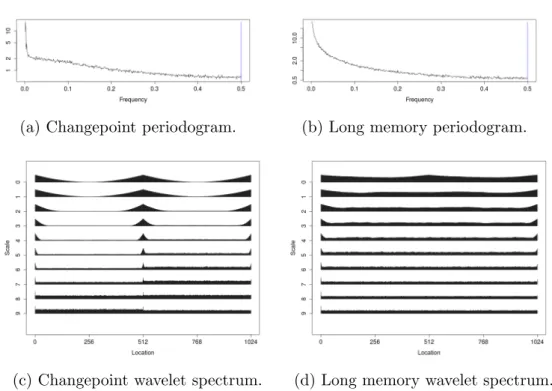
(a) Changepoint periodogram. (b) Long memory periodogram.

(c) Changepoint wavelet spectrum. (d) Long memory wavelet spectrum.

Figure 3.1: Empirical periodogram and wavelet spectrum averaged over 500 real-izations.

The ambiguity present between diagnostics of the competing models given in Equation (3.1) and (3.2) can cause issues in identifying the correct model. Figure 3.1 shows the average empirical periodograms from realisations of long memory (ARFIMA(0,0.4,0)) and changepoint (AR(1), λ= 0.5, φ1 = 0.1,φ2 = 0.4, µ1 = 0,

µ2 = 1) models. It can be seen that the periodogram for the changepoint model

has a pole at zero and shows similar behaviour to that of long memory.

Before discussing the wavelet spectrum, we provide a brief background to wavelets and the specific spectrum we propose to use.

Wavelets capture properties of the data through a location-scale decomposition using compactly supported oscillating functions. Through dilation and translation, a wavelet is applied across a number of a scales and locations to capture behaviour occurring over different parts of a series. Further information on them and their application can be found in Daubechies (1992) and Nason (2010). In this work we use the model framework of the Locally Stationary Wavelet process which provides a stochastic model for second order structure using wavelets as building blocks.

(39)

We follow the definition in Fryzlewicz and Nason (2006) for a Locally Stationary Wavelet (LSW) process.

Definition 3.1. Define the triangular stochastic array {Xt,N}N

−1

t=0 which is in the

class of LSW processes given it has the mean-square representation

Xt,N = ∞ X j=1 X k Wj k n ψj,k−tξj,k,

where j ∈ 1,2, . . . and k ∈ Z are scale and location parameters respectively, ψj =

(ψj,0, . . . , ψj,Lj−1)are discrete, compactly supported, real-valued non-decimated wavelet vectors of support length Lj. If the ψj are Daubechies wavelets Daubechies (1992) then Lj = (2j −1)(Nh −1) + 1 where Nh is the length of the Daubechies wavelet filter, finally the ξj,k are orthonormal, zero-mean, identically distributed random variables. The amplitudes Wj(z) : [0,1]→R at each j ≥1 are time varying, real-valued, piecewise constant functions which have an unknown (but finite) amount of jumps. The constraints on Wj(z)are such that if Pj are constants representing the total magnitude of jumps in W2

j(z), then the variability of Wj(z) is controlled by • P∞ j=12jPj <∞, • P∞ j=1W 2 j(z)<∞ uniformly in z.

Note that we apply this framework to our models given in Equations 3.1 and 3.3 as both are stationary models under the assumption thatd∈(0,0.5). Thus by Wold’s Decomposition Theorem (Geary, 1956), which states that any stationary model can be represented as a Moving Average (MA) model with infinite param-eters, we can represent the ARFIMA model as an MA(∞). Further, by Nason et al. (2000) it is shown that any MA model can be represented in as an LSW and thus are applicable here.

(40)

ampli-tudes and as such the Evolutionary Wavelet Spectrum can be defined as Sj k N = Wj k N 2

which changes over both scale (frequency band) j and location (time) k.

Considering both scale and location, the two dimensions allow the differences between the proposed models to be seen. Examples of the differences in these spectra are given in Figure 3.1 for both the changepoint and long memory models. To interpret the wavelet spectrum: scale corresponds to frequency bands with high frequency at the bottom to low frequency at the top. Further details on the spectrum and its applicability can be found in Fryzlewicz and Nason (2006), Nason (2010) and Killick et al. (2013). Note that there is a clear difference between the wavelet spectra of the two models with the changepoint model being piecewise stationary (pre and post change), with the change occurring in the spectrum where the change occurs in the data. In contrast the long memory model remains flat across each scale and time reflecting the stationarity of the original series.

Due to the fact that the wavelet spectrum gives a distinction between the two models we propose to use this as the basis for our inference regarding the most appropriate model. Whilst the Fourier spectrum could be used here as in Janacek et al. (2005), we choose to use the Evolutionary Wavelet Spectrum. As shown in Figure 3.1 this is advantageous for characterising the non-stationarity changepoint data due to the Scale-Location transformation used. This is since the Wj(z) are

constant for stationary models, but for non-stationary models the break in the second order structure of the original data causes breaks in the wavelet spectra, as described in Cho and Fryzlewicz (2012).

In the next section we detail how to use the wavelet spectrum of the two models in a classification procedure.

(41)

3.2.3 Classification

Testing whether a long memory or changepoint model is more appropriate whilst under model uncertainty comes with the hazard of mis-specification. A formal hypothesis test places assumptions on the underlying model in both the null and alternative, but the allocation of the null is hazardous - should the changepoint model be the null or alternative? It would be entirely feasible to choose the changepoint model as the null model, not reject H0 and then flip to have the long memory model as the null model and also not reject H0. Given the absence

of a clear null model, which result to proceed with is unclear. Instead it may be preferable to quantify the evidence for each model separately. A classification method such as the one proposed here gives a candidate series a measure of distance from a number of groups, which can then be used to select the most appropriate group.

In the previous subsection it was demonstrated that the wavelet spectrum can be used to distinguish the changepoint model from the long memory model, and the classifier proposed here builds on this. However, to begin a classification method must first ‘teach’ itself on the structure of the classes through sets of training data. These are data sets already determined to be in each category and are the basis for calculating the distances from each group. This previous knowledge allows for determination of patterns and features of each category (that are unique from other categories) for comparison to the candidate data set. A common example is the spam filter on mailboxes, which is trained on previous spam emails so that it can classify if a new email that arrives is spam or not. The decision is made by comparing it to a number of patterns already determined to be features in spam email for example, short messages or hidden sender identities. Further information on classification methods and training them can be found within Michie et al. (1994).

In our example we only have a single data set of length n, the classifier has no previous information to train on. To remedy this we create training data through

(42)

simulation. Given a candidate series we first fit the competing models in Equations (3.1) and (3.2) choosing the best fit for each model. For the changepoint model the best fit uses the ARMA likelihood within the PELT multiple changepoint frame-work to identify multiple changes in ARMA structure (Hyndman and Khandakar, 2008; Killick et al., 2012). When considering fitted long memory models, a number of ARFIMA models are fitted (Veenstra, 2012) and selection occurs according to Bayesian Information Criterion (following Beran et al. (1998)).

Following the identification of the best changepoint and long memory mod-els, the training data is then simulated as (Monte Carlo) realisations from these, denoted by

Xg_m=X_i,mg

i=1,2,...,n m= 1,2, . . . , M.

g = 1,2.

where the group, g = 1 for changepoint simulations and g = 2 for long memory simulations,M is the number of simulated series andnis the length of the original series. Note that we are not sampling from the original series, we are generating realizations from the fitted models.

Now we have the training data and the observed data, denotedXo, a measure of distance of the observed data from each group is calculated. As discussed previously we will use a comparison of their evolutionary wavelet spectra as the distance metric. Before detailing the metric, we first define the estimated wavelet spectrum of the original series as

ˆ

So =nSˆ_koo

k=1,2,...n∗J

where we remove the index over scale j by concatenating scales, hence k = 1,2, . . . n∗J, where J =blog₂(n)c. Similarly we define the spectra for each simu-lated series: ˆ Sg_m = n ˆ S_k,mg o k=1,2,...n∗J.

(43)

To obtain a group spectra, an average is then taken over the M simulated series at each position of each scale for each group,

¯ Sg = ( 1 M M X m=1 ˆ S_k,mg ) k=1,2,...n∗J .

Based on these spectra the distance metric proposed is a variance corrected squared distance, across all spectral coefficients as proposed in Krzemieniewska et al. (2014), Dg = M (M+ 1) n∗J X k=1 ( ˆS_ko−S¯_kg)2 PM m=1( ˆS g k,m−S¯ g k)2 (3.3)

Note that the variance correction occurs within the denominator to account for potentially different variability seen across simulations for each group. This is modified from Krzemieniewska et al. (2014) to allow different variances within each group. The theoretical consistency of the classification was shown in Theo-rem 3.1 from Fryzlewicz and Ombao (2009) where the error for misclassifying two spectra {S_k(1)}k and {S

(2)

k }k (whose difference summed over k is larger than CN)

is bounded by O N−1_log3

2N +N1/

{2 log2(a)−1}−1log2

2N

. However this result re-quires a short memory assumption that is clearly not satisfied for our long memory processes. Thus we prove a similar bound under the assumption that the spectra are created from ARFIMA processes. We first replicate the required assumptions from Fryzlewicz and Ombao (2009) for completeness:

Assumption 3.2. (Assumption 2.1 from Fryzlewicz and Ombao (2009))

The set of those locationszwhere (possibly infinitely many) functionsSj(z)contain a jump is finite. In other words, letB:={z :∃jlimu→z−S_j(u)6=∃jlim_u_→_z+}. We assume B := #B <∞.

Assumption 3.3. (Assumption 2.2 from Fryzlewicz and Ombao (2009))

There exists a positive constantC1 such that for all j, Sj(z)≤C12j.

Theorem 3.4. Suppose that Assumptions 3.2 and 3.3 hold, and that the constants

Pj from Definition 3.1 decay as O(aj) for a > 2. Let S

(1)

j (z) and S

(2)

(44)

non-identical wavelet spectra from Changepoint ARFIMA processes. Let I_k,N(J) be the wavelet periodogram constructed from a process with spectrum S(1)(z), and let

L(_k,Nj) be the corresponding bias-corrected periodogram, with J∗ = log₂N. Let

X

j,k n

S_j(1)(k/N)−S_j(2)(k/N)o2 =O(N).

The probability of misclassifying L(_k,Nj) as coming from a process with spectrum

S_j(2)(z) can be bounded as follows:

P(D1 > D2) =O

log2₂NhN−1+N(2 log21a−1)−1 i

Proof. The proof is given in Appendix 3.6.1.

A summary of the proposed procedure is given in Algorithm 1.

3.3 Simulation Study

To test the empirical accuracy of our proposed approach, simulations were con-ducted over a number of models. Here, these models are chosen over a number of parameter magnitudes and combinations to show the effectiveness of the ap-proach outlined in Section 3.2. A number of these models also appear in Yau and Davis (2012) which uses a likelihood-ratio method to test the null hypothesis of a changepoint model. As part of their notation they introduce λ which represents the location in the series where the changepoint occurs, such that λ = τ_n. Their results for these models are correspondingly given as a comparison.

For each model given in the tables below, 500 realisations of each model were generated and classified, using M = 1000 training simulations for each fit. For computational efficiency, the maximum order of the fitted models are constrained to p, q ≤ 1. Three different time series lengths were computed for each model;

n= 512,1024,2048. It is expected that as a series grows larger, more evidence of long memory features will become prevalent, and as such the effect of length of

(45)

1 Initialization:

2 X:{X_i}n_i₌₁ observed series. 3 n : Length of series

4 M : Number of bootstrap simulations 5 S¯1, S¯2 : Empty Spectra 1, 2.

6

Algorithm:

1. Fit: M1 - best changepoint model (Equation (3.1)) to X.

2. Fit: M2 - best long memory model (Equation (3.2)) to X.

3. Calculate training spectra

for m= 1,2, . . . , M do

Simulaten observations fromM1, denote as Y1

Calculate Evolutionary Wavelet SpectraSˆ1_m of Y1

LetS¯1 =S¯1+Sˆ1_m

Simulaten observations fromM2, Y2

Calculate Evolutionary Wavelet SpectraSˆ2_m of Y2

LetS¯2 =S¯2+Sˆ2_m

end

4. Calculate the average Evolutionary Wavelet Spectra for each group

¯

S1 = S_M¯1, S¯2 = S_M¯2.

5. Calculate Evolutionary Wavelet Spectrum of X,Sˆo. 6. Compute the distance D1, D2, betweenSˆ

o

and S¯1, S¯2 respectively (Equation (3.3)).

Output: Distances D1, D2.

(46)

series on accuracy is investigated.

We have used n = 2J as the length of the series as the wavelet decomposition software in Nason (2016b) requires that the series transformed is of dyadic length. This is not a desirable trait as data sets come in many different sizes. Thus we over-come this using a standard padding technique described in Nason (2010) that adds 0’s to the left of each series until the data is of length 2J_{. The extended wavelet}

coefficients are then removed before calculating the distance metric. Finally, we use the Haar Wavelet across all simulations.

3.3.1 Changepoint Observations

Model Parameters Classification Rate (n =) Y&D LR (n=)

Ref λ µ φ1 θ1 φ2 θ2 512 1024 2048 500 1000 1 0.5 1 0.1 0.3 0.4 0.2 1.00 1.00 1.00 0.99 0.97 2 0.5 2 0.1 0.3 0.4 0.2 1.00 1.00 1.00 0.95 0.93 3 0.5 1 0.1 0.3 0.8 0.2 1.00 1.00 1.00 0.97 0.99 4 0.5 2 0.1 0.3 0.8 0.2 1.00 1.00 1.00 0.94 0.95 5 0.7 1 0.1 0.3 0.8 0.2 1.00 1.00 1.00 0.94 0.94 6 0.7 2 0.1 0.3 0.8 0.2 1.00 1.00 1.00 0.91 0.93

Table 3.1: Changepoint observations results with Likelihood Ratio results com-parison taken from Yau and Davis (2012).

For the changepoint models we used the simulations given in Yau and Davis (2012). Table 3.1 gives the parameters used in Equation (3.1) along with the correct classification rate. The results show that if the data follows a changepoint model then we have a 100% classification rate. A movement of the changepoint to a later part of the series, as in models 5 and 6, does not appear to have an effect upon classification rates unlike for the Yau and Davis method. It is not really a surprise that we are receiving 100% classification rates as if a changepoint occurs then it is a clear feature within the spectrum.

It should be noted that as the Yau and Davis method is a hypothesis test we would expect results around 0.95 for a 5% type I error.

(47)

3.3.2 Long Memory Observations

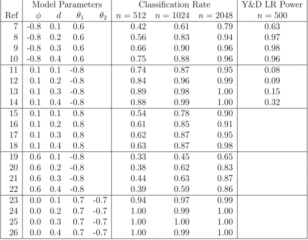
Model Parameters Classification Rate Y&D LR Power

Ref φ d θ1 θ2 n = 512 n = 1024 n= 2048 n= 500 7 -0.8 0.1 0.6 0.42 0.61 0.79 0.63 8 -0.8 0.2 0.6 0.56 0.83 0.94 0.97 9 -0.8 0.3 0.6 0.66 0.90 0.96 0.98 10 -0.8 0.4 0.6 0.75 0.88 0.96 0.96 11 0.1 0.1 -0.8 0.74 0.87 0.95 0.08 12 0.1 0.2 -0.8 0.84 0.96 0.99 0.09 13 0.1 0.3 -0.8 0.89 0.98 1.00 0.15 14 0.1 0.4 -0.8 0.88 0.99 1.00 0.32 15 0.1 0.1 0.8 0.54 0.78 0.90 16 0.1 0.2 0.8 0.61 0.85 0.91 17 0.1 0.3 0.8 0.62 0.87 0.95 18 0.1 0.4 0.8 0.63 0.87 0.98 19 0.6 0.1 -0.8 0.33 0.45 0.65 20 0.6 0.2 -0.8 0.38 0.62 0.83 21 0.6 0.3 -0.8 0.44 0.63 0.87 22 0.6 0.4 -0.8 0.39 0.59 0.86 23 0.0 0.1 0.7 -0.7 0.94 0.97 0.99 24 0.0 0.2 0.7 -0.7 1.00 0.99 1.00 25 0.0 0.3 0.7 -0.7 1.00 1.00 1.00 26 0.0 0.4 0.7 -0.7 1.00 0.99 1.00

Table 3.2: Long memory observations results with Likelihood Ratio results com-parison taken from Yau and Davis (2012).

In contrast to the changepoint models, the classification of a long memory model is expected to be less clear. This is due to the variation within the wavelet spectrum of long memory series that could be interpreted as different levels and hence a changepoint model would be more appropriate. To demonstrate the effect of the classifier on long memory observations, a larger number of models were considered. We simulated long memory models with differing levels of long memory as measured by the d parameter, values close to 0 are closer to short memory models and values close to 0.5 are stronger long memory models (values>0.5 are not stationary and thus not considered).

The results in Table 3.2 give an indication of the accuracy of the classifier in a number of different situations. Overall, as the length of the time series increases we see an increase in classification accuracy. This is to be expected as evidence of

(48)

long memory will be more prevalent in longer series. Similarly as we increase the long memory parameterd from 0.1 to 0.4 we improve the classification rate.

Some interesting things to note include, when there are strong AR parameters (φ) such as models 7-10 and 19-22 we require longer time series to achieve good classification rates. However, in contrast if there are strong MA components as in the remaining models the classifier performs better. A larger effect is found when the MA parameter is negative, seen through models 11-14 where the classifier performs strongly even at n = 512. This effect is further exemplified by models 23-26 which include a further MA parameter and achieve near 100% classification atn= 512. Here the maximum used p, q was 2.

Comparing our results to that of Yau and Davis we note that the opposite performance is seen. For the likelihood ratio method there is high power for models with strong AR components and poor performance for strong MA components. Notably the strong MA performance is much worse than our method on the strong AR components.

3.4 Application

To further demonstrate the usage of our approach, two applications to real data are given in this section. The first is an economics example based on US price inflation and this is followed by financial data on stock cross-correlations. A sensitivity analysis was conducted over the possible maximum values of p, q. It was found that no additional parameters were required beyond maximump, q = 4, thus these results are presented here.

3.4.1 Price Inflation

US price inflation can be determined using the GDP index. The dataset used here is available from the Bureau of Economic Analysis, based on quarterly GDP indexes, denotedPt, from the first quarter of 1947 to the third quarter of 2006 (227

(49)

data points). Price inflation is calculated asπt = 400 ln(Pt/Pt−1) (thus n = 226).

A plot of the inflation is given below in Figure 3.2a. Studies of the persistence of this data have been conducted to determine the level of dependence within the series. A high amount of persistence, indicating long memory, was found in Pivetta and Reis (2007). However Levin and Piger (2004) found a structural break, which when accounted for showed the series to have low persistence, indicating the presence of changepoints with short memory segments. Applying our classification approach to this series will give an additional indication as to which model is statistically more appropriate.

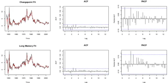
The parameters of the fitted changepoint and long memory models are given in Table 3.3. Diagnostic autocorrelation and partial autocorrelation function plots are given in Figure 3.3. The level shifts are given in respect to their position in the series, but correspond to 1951 Q3, 1962 Q4, 1965 Q2, 1984 Q2. The classifier returns a changepoint classification for this series.

3.4.2 Stock Cross Correlations

Stock Cross Correlation data has been obtained from the supplementary material of Chiriac and Voev (2011). The data consists of Open to Close stock returns for 6 companies from January 1st 2001 to 30th July 2008 (n = 2156). The data is first transformed using a Fisher Transformation, then correlations are calculated between each stock. Here analysis will look at the correlation between American Express and Home Depot.

This data has been analysed previously by Bertram et al. (2013) to determine between fractional integration (long memory behaviour) and level shifts and is given in Figure 3.2b. Parameters for the models fitted by the algorithm are also in Table 3.3. It can be seen that one of the AR coefficients is close to 1 indicating an element of non-stationarity, however we conducted a test of stationarity on this segment using the locits R package (Nason, 2016a) which implements the test of stationarity from Nason (2013) (no rejections) and also the fractal R

(50)

package (Constantine and Percival, 2016) which implements the Priestley-Subba Rao (PSR) test (Priestley and Rao, 1969) (time varying p-value 0.061). This coupled with autocorrelation and partial autocorrelation function plots given in Figure 3.4 means we conclude that the segment is stationary. Here the estimated changepoints at times 715, 841, 847 and 896 correspond 15/12/2002, 20/04/2003, 26/04/2003 and 14/06/2003. The distance scores given by the classifier indicate a strong preference for long memory over changepoints. This result stands against that found in Bertram et al. (2013) which indicated a preference for a model with similarly 4 changepoints. The difference is likely due to the fact that in Bertram et al. (2013) the changepoint model does not contain any short memory dependence and we have shown here that if that short memory structure is correctly taken into account within the sub-series then the series shows greater evidence of long memory properties.

(51)

(a) Time series of US Price Inflation.

(b) Time series of the Cross Correlations of American Express and Home Depot.

(52)

Long Memory Mo del Score Changep oin t Mo del Score Data Inflation Sto ck ARFIMA(4 , 0 , 0) φ = (0 . 30 , 0 . 20 , 0 . 20 , − 0 . 16) d = 0 . 31 µ = 3 . 29 ARFIMA(1 , 0 , 1) φ = 0 . 30 θ = 0 . 58 d = 0 . 47 , µ = 0 . 35 40147 ₁₂₁₂₈ AR(1) φ= 0 . 68 , τ = 18 , µ = 0 AR(1) φ= 0 . 63 , τ = 63 , µ = 1 . 70 ARMA(2 , 1) φ = ( − 0 . 43 , − 0 . 33) θ = 0 . 47 , τ = 73 , µ = 1 . 69 AR(1) φ= 0 . 82 , τ = 149 , µ = 5 . 43 AR(3) φ = (0 . 60 , 0 . 19 , 0 . 18) τ = 226 , µ = 0 ARMA(4 , 4) φ = ( − 0 . 05 , − 0 . 002 , 0 . 07 , 0 . 94) θ = (0 . 17 , 0 . 14 , 0 . 04 , − 0 . 83) τ = 715 , µ = 0 . 31 AR(1) φ= 0 . 29 , τ = 841 , µ = 0 . 42 ARMA(2 , 1) φ = (0 . 09 , 0 . 09) θ = − 0 . 58 , τ = 847 , µ = 0 . 30 MA(1) θ= − 0 . 72 , τ = 896 , µ = 0 . 50 ARMA(3 , 1) φ = (1 . 12 , − 0 . 06 , − 0 . 07) θ = − 0 . 90 , τ = 2156 , µ = 0 . 35 Segmen t 1 Segmen t 2 Segmen t3 Segmen t 4 Segmen t 5 38750 Segmen t 1 Segmen t 2 Segemn t 3 Segmen t 4 Segmen t 5 5348047 T able 3.3: Mo del fits and scores for US Inflation (I n flation) and Sto ck Cross-Correlations (S to ck). Bold scores are the minim um. Eac h segmen t ending at τ is separated b y a dotted line.

(53)

Figure 3.3: Inflation diagnostics. (Top) Left: Original data with fitted changepoint model; Middle: Autocorrelation function of changepoint model residuals; Right: Partial autocorrelations of changepoint model residuals. (Bottom) Left: Original data with fitted long memory model; Middle: Autocorrelation function of long memory model residuals; Right: Partial autocorrelations of long memory model residuals.

Figure 3.4: Stock diagnostics. (Top) Left: Original data with fitted changepoint model; Middle: Autocorrelation unction of changepoint model residuals; Right: Partial autocorrelations of changepoint model residuals. (Bottom) Left: Original data with fitted long memory model; Middle: Autocorrelation function of long memory model residuals; Right: Partial autocorrelations of long memory model residuals.

Detecting patterns in Time Series Data with applications in Official Statistics