Multi-view Subspace Learning for Large-Scale Multi-Modal Data Analysis

(1)

MULTI-VIEW SUBSPACE LEARNING FOR

LARGE-SCALE MULTI-MODAL DATA

ANALYSIS

Faculty of Information Technology and Communication Sciences Master of Science Thesis August 2019

(2)

ABSTRACT

Kateryna Chumachenko: VIEW SUBSPACE LEARNING FOR LARGE-SCALE MULTI-MODAL DATA ANALYSIS

Master of Science Thesis Tampere University

Master’s Degree Programme in Information Technology Major: Data Engineering and Machine Learning August 2019

Dimensionality reduction methods play a big role within the modern machine learning tech-niques, and subspace learning is one of the common approaches to it. Although various methods have been proposed over the past years, many of them suffer from limitations related to the uni-modality assumptions on the data and low speed in the cases of high-dimensional data (in linear formulations) or large datasets (in kernel-based formulations). In this work, several methods for overcoming these limitations are proposed.

In this thesis, the problem of the large-scale modal data analysis for single- and multi-view data is discussed, and several extensions for Subclass Discriminant Analysis (SDA) are proposed. First, a Spectral Regression Subclass Discriminant Analysis method relying on the Graph Embedding-based formulation of SDA is proposed as a way to reduce the training time, and it is shown how the solution can be obtained efficiently, therefore reducing the computational requirements. Secondly, a novel multi-view formulation for Subclass Discriminant Analysis is proposed, allowing to extend it to data coming from multiple views. Besides, a speed-up approach for the multi-view formulation that allows reducing the computational requirements of the method is proposed. Linear and nonlinear kernel-based formulations are proposed for all the extensions.

Experiments are performed on nine single-view and nine multi-view datasets and the accu-racy and speed of the proposed extensions are evaluated. Experimentally it is shown that the proposed approaches result in a significant reduction of the training time while providing compet-itive performance, as compared to other subspace-learning based methods.

Keywords: subspace learning, kernel methods, dimensionality reduction, spectral regression, subclass discriminant analysis

(3)

PREFACE

The work in this thesis was conducted in the Multimedia Research Group in the Depart-ment of Computing Sciences in the Faculty of Information Technology and Communica-tion Sciences in Tampere University in 2019.

I would like to express my sincere gratitude to Prof. Moncef Gabbouj, Assoc. Prof. Alexandros Iosifidis and Dr. Jenni Raitoharju for giving me the opportunity to work as a research assistant within the group and providing constant guidance and support through-out the work process.

Besides, I would like to thank all the members of Multimedia Research Group for creating such a nice and motivational work atmosphere.

In addition, I would like to thank my family for their support throughout my studies and my life in general.

Tampere, 1st August 2019

(4)

LIST OF FIGURES

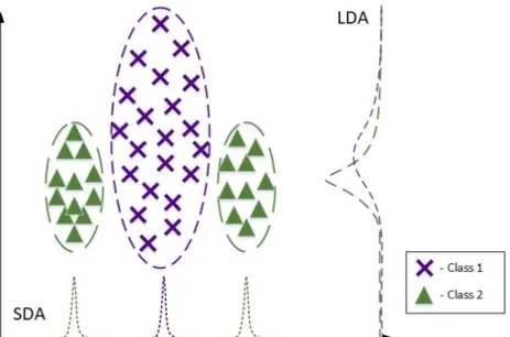
1.1 Subclass data when projected to LDA subspace and SDA subspace . . . . 3

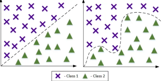
2.1 Linear decision boundary vs. nonlinear decision boundary. . . 5

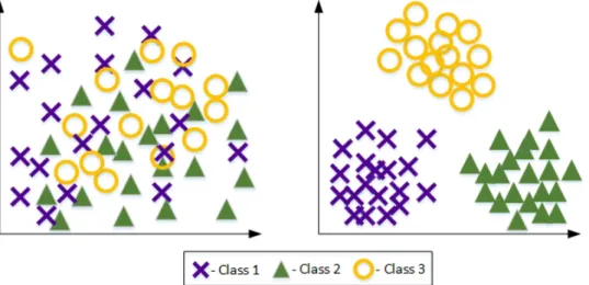
2.2 Data before and after LDA projection. . . 7

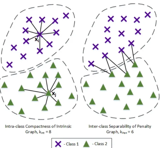
2.3 Marginal Fisher Analysis graphs adjacency relationships. . . 12

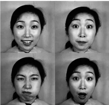
4.1 Example of images from Jaffe dataset. . . 39

4.2 Example of images from Cohn-Kanade dataset. . . 40

4.3 Example of images from Extended Yale-B dataset. . . 40

4.4 Example of images from SoF dataset. . . 41

4.5 Example of images from Caltech-101 dataset. . . 43

(6)

LIST OF TABLES

3.1 Structure of the between-class Laplacian matrix in SDA. . . 29

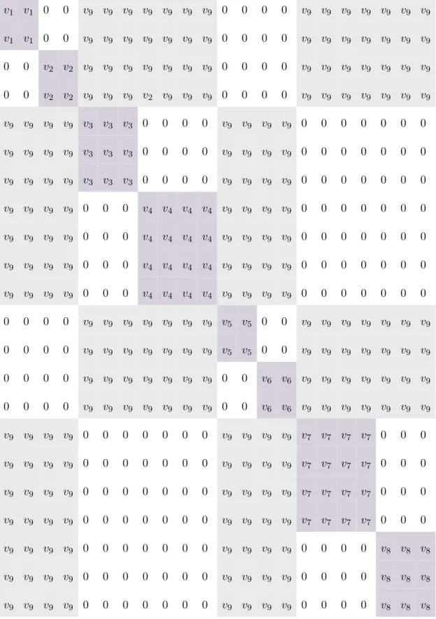
3.2 Structure of the between-class Laplacian matrix in multi-view SDA. . . 35

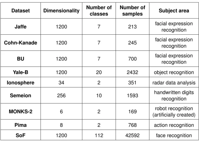
4.1 Summary of single-view datasets. . . 42

4.2 Summary of multi-view datasets. . . 45

4.3 Classification results of linear methods in single-view datasets: accura-cy/number of clusters per class. . . 46

4.4 Classification results of linear methods in single-view datasets: training time (in sec). . . 46

4.5 Classification results of kernel methods in single-view datasets: accura-cy/number of clusters per class. . . 47

4.6 Classification results of kernel methods in single-view datasets: training time (in sec). . . 47

4.7 Classification results of linear methods in multi-view datasets: accura-cy/number of clusters per class. . . 48

4.8 Classification results of linear methods in multi-view datasets: training time (in sec). . . 48

4.9 Classification results of kernel methods in multi-view datasets: accura-cy/number of clusters per class. . . 49

4.10 Classification results of kernel methods in multi-view datasets: training time (in sec). . . 49

(7)

LIST OF ABBREVIATIONS

CDA Clustering Discriminant Analysis

KCDA Kernel Clustering Discriminant Analysis KSDA Kernel Subclass Discriminant Analysis KSMFA Kernel Subclass Marginal Fisher Analysis LDA Linear Discriminant Analysis

MFA Marginal Fisher Analysis

MvMDA Multi-view Modular Discriminant Analysis NPT Nonlinear Projection Trick

PCA Principal Component Analysis RBF Radial Basis Function

SDA Subclass Discriminant Analysis SGE Subclass Graph Embedding SMFA Subclass Marginal Fisher Analysis

SMvDA Standard Multi-view Discriminant Analysis SRDA Spectral Regression Discriminant Analysis fastSDA Fast Subclass Discriminant Analysis mvSDA Multi-view Subclass Discriminant Analysis

(8)

1 INTRODUCTION

Availability of the large amounts of data in the modern world dictates the development of new technologies for processing and analysing it, giving rise to the field of machine learning. In the past years, machine learning has been applied to solve problems in many subject areas, including image processing [38, 61], audio and speech analysis [3, 20], human action recognition [17], etc. In many areas, such as face recognition or object detection, machine learning-based methods are the dominant approach to solving prob-lems [45, 47, 48, 51]. Although the presence of rich data from different sources allows improving the accuracy of the algorithms, it also raises issues related to their compu-tational requirements. In this thesis, we study a subfield of machine learning, namely, subspace learning, and propose several extensions for speeding-up and improving the accuracy of existing methods.

The goal of machine learning is to estimate the parameters of a mathematical model to perform a specific task without using explicit instructions, but relying on the patterns in the data, from which it learns. The data, in this case, is represented by a matrix or a tensor, i.e., multiple samples described by one or multiple features. Intuitively it might seem that a larger amount of features should result in better accuracy of the model, which is true only up to a certain point: when the dimensionality of data becomes too high, the accuracy of the model drops, as the data representation becomes sparse, i.e., there are not enough samples to capture enough possible combinations of the features. This phenomenon is known as the ’curse of dimensionality’. Another limitation that comes with high dimen-sionality is the high computational complexity that results in low processing speed. These issues resulted in the formation of a research area referred to as dimensionality reduction. Dimensionality reduction methods aim to find such a representation of data that would result in a lower dimensionality than that of original data while preserving the ’meaning-fulness’ of data. The ’meaning’meaning-fulness’ can be defined by different criteria, e.g., some methods seek representation with the highest variance, while others a representation, where data belonging to different classes lies far from each other, while classes are com-pact.

Machine learning methods can be divided into supervised and unsupervised ones. Su-pervised machine learning, also referred to as ’learning with a teacher’, relies on the ground truth labels present for all data samples in the training set. Examples of super-vised machine learning problems are regression and classification. Unsupersuper-vised learn-ing methods do not rely on the ground truth labels of data but try to find certain patterns

(9)

in the data. Clustering is one of the examples of unsupervised learning. In this thesis, we focus on supervised dimensionality reduction methods that aim at classification problems. One of the common dimensionality reduction approaches is subspace learning, which aims to find a projection subspace of a lower dimensionality for the data while ensuring that a certain criterion holds for the data projected onto the subspace. Examples of subspace learning methods include Principal Component Analysis (PCA) [16], Linear Discriminant Analysis (LDA) [57, 60], Subclass Discriminant Analysis (SDA) [66], etc. Linear Discriminant Analysis is one of the most well-known subspace learning methods designed primarily for classification problems. LDA defines an optimal projection space as the one where the distances between the different class means are maximal, while the classes are compact. The solution is based on the assumption that each class follows a unimodal Gaussian distribution. Several limitations come from this assumption:

• limited dimensionality of the learned space, as it is limited by the rank of the between-class scatter matrix, which is bounded by the number of between-classes - 1

• poor performance on multi-modal datasets, as LDA assumes that data of each class follows a unimodal Gaussian distribution

• high computational complexity in high-dimensional datasets, as the solution is given by the eigendecomposition of a large matrix.

Multiple approaches to overcoming these limitations have been proposed [13, 26, 27, 28, 66]. One of the proposed approaches is the Subclass Discriminant Analysis, that relaxes the assumptions on the unimodal distribution of each class by representing it with several subclasses and formulating the criterion accordingly. This allows to obtain better perfor-mance on the real-world data, which does not generally follow unimodal distributions, and potentially obtain higher dimensionality, as the rank of the between-class scatter matrix becomes higher, as shown in the next chapters. The benefits of using SDA can be seen from Fig. 1.1, where the data of class 2 follows 2 disjoint distributions. As the means of two classes lie close to each other, LDA fails to find a subspace that would discriminate the classes well, while SDA succeeds, as can be seen from the figure.

However, the limitation of the high computational complexity remains valid, as the solu-tion still requires an eigendecomposisolu-tion of a large matrix. To overcome this limitasolu-tion, multiple solutions have been proposed over the past years, including incremental learn-ing solutions [34], approximate solutions [24], and speed-up solutions [9, 25, 29, 30, 59]. In this thesis, a speed-up extension for overcoming this limitation is proposed.

So far we have considered the methods that rely on one representation of a set of sam-ples. Such methods are known as single-view methods. Inspired by the human percep-tion of the world, that is not only based on one source of informapercep-tion but on a combi-nation of the audio, visual, and tactile signals, etc., various multi-view learning methods have been proposed [10, 32, 63, 64, 67]. Such methods refer to the problems where multiple descriptions of the same set of samples are available. These descriptions can come from different domains, e.g., in the problem of the classification of a video based

(10)

Figure 1.1.Subclass data when projected to LDA subspace and SDA subspace

on its audio and visual signals, or from different features of the same domain, e.g., in the problem of the classification of audio signal based on MFCC and ZCR. Different views can be also represented by the same type of features that are obtained from different data corresponding to the same sample, e.g., in the problem of person re-identification from multiple cameras.

Multiple extensions of LDA to multi-view problems have been proposed [10, 32, 65], but they mostly assume unimodality of classes in each view. In this thesis, an approach for overcoming this limitation by introducing a multi-view extension to Subclass Discriminant Analysis is proposed, and it is shown how the solution can be obtained in a fast and efficient way [15].

In order to address the issues of already existing methods as outlined earlier, we formu-late the research problem of this work as the development of a method that would satisfy the following requirements:

• relax the assumptions of unimodality of each class

• be computationally efficient in both linear and non-linear formulations

• have the possible dimensionality higher than the number of classes−1

• be able to extend to multi-view data.

This thesis is organized as follows: in chapter 2, the previous work relevant to the further development of the proposed extensions is described, including the relevant subspace learning methods, kernel methods, and speed-up approaches. In chapter 3, the pro-posed extensions for Subclass Discriminant Analysis are described. In chapter 4, the experimental setup along with the datasets used for evaluation of the methods are de-scribed and the results are reported. In chapter 5, conclusions are made regarding the proposed approaches.

(11)

2 THEORETICAL BACKGROUND

2.1 Subspace Learning

In this section, the related work in the area of subspace learning is described. The goal of subspace learning methods is to find a subspace of lower dimensionality, projection onto which would result in the low-dimensional data while satisfying some criterion defined for the original data. Let X = [x1,x2, ...,xN]be a set ofN D-dimensional vectors in some

spaceRD, and let each vectorxi correspond to a class labelci. Using these notations, we can define the problem of dimensionality reduction as finding a feature space, defined by the projection matrix W, such that its dimensionality is smaller than that of original space, and data belonging to different classes lies far from each other when projected onto it, while samples of the same class lie close to each other.

Prevailing part of the subspace learning methods find such a feature space by optimiz-ing the Fisher-Rao’s criterion [19, 46], that is defined over two symmetric positive semi-definite matrices, referred to as within-class scatter matrixSw and between-class scatter matrixSb: J(W) =argmin W T r(WTSwW) T r(WT_S bW) . (2.1)

In other words, we want to minimize the within-class scatter of the data and maximize the between-class scatter while ensuring the orthogonality of the projection matrix.

The solution to the optimization problem in (2.1) is obtained by solving a generalized eigendecomposition problem [31]:

Sww=λSbw, (2.2)

and the projection matrixW is obtained by choosing the eigenvectors corresponding to minimal eigenvalues. The data in the feature space is obtained by a linear projection:

yi =WTxi. (2.3)

Differences between various subspace learning methods primarily lie in the definitions of the between-class and the within-class scatter matrices. Further in this chapter, we will focus on different approaches taken in this area.

(12)

2.2 Linear and Nonlinear Learning

Being based on a linear projection, linear subspace learning approach described in the previous section assumes linear separability of data and cannot take into account possi-ble nonlinearities that are often present in the real-world data. An example of such data is outlined in Fig. 2.1. To address this issue, multiple approaches have been taken, includ-ing kernel methods, neural network-based methods, random projections-based methods, etc. In this section, we focus on two of the commonly used approaches: a kernel-based approach that allows to learn the nonlinear decision boundaries without explicitly mapping the data to the nonlinear space, and the Nonlinear Projection Trick approach.

Figure 2.1. Linear decision boundary vs. nonlinear decision boundary.

The idea of the two approaches lies in the following: rather than finding a linear projection of the data inX ∈_RD _{directly, our goal is to first map it to some nonlinear feature space}

F. The nonlinear feature space is defined by some nonlinear functionϕ(), i.e.,ϕ(xi)∈ F. The dimensionality of F depends on the choice of the nonlinear function and can be infinite. A linear projection is then defined inF, i.e. yi=WTϕ(xi).

2.2.1 Kernel Trick

The explicit mapping of each sample inXto its imageϕi=ϕ(xi)raises issues related to the arbitrary dimensionality of F, which can be infinite. To address this issue and avoid the explicit learning of nonlinear function ϕ() and mapping of X to Φ = ϕ(X) directly, kernel functions can be used. A kernel functionk()is defined over a pair of samples in Xand maps their inner product inRD to the corresponding inner product of their images inF :k(x1,x2) =ϕ(x1)Tϕ(x2). Thus, formulation of the subspace learning problem in a

way that only relies on the inner products of data, rather than on the data directly, allows obtaining an efficient nonlinear solution.

(13)

The kernel matrixKof size N ×N is, therefore, defined asKij = k(xi,xj). It is trivial to see that sincek(xi,xj) =ϕ(xi)Tϕ(xj),K=ΦTΦ, whereΦ= [ϕ(x1), ϕ(x2), ..., ϕ(xN)]. The kernel matrix K is generally assumed to be non-singular, while in the case of a singular matrix it is generally regularized as K′ = K+δI, where δ is a regularization parameter. According to the Representer Theorem [49], W can be represented as a linear combination of data inF:

W=ΦA. (2.4)

Hence,yi =WTϕ(xi) =ATΦTϕ(xi) =ATki.

2.2.2 Nonlinear Projection Trick

Although kernel methods are widely used in machine learning problems where nonlin-earity is required, there exist many optimization problems which are impossible to for-mulate solely with inner products, making the application of kernel trick impossible. For such problems, an approach referred to as Nonlinear Projection Trick (NPT) has been proposed [35]. In NPT, data samples are mapped to a nonlinear space of reduced di-mensionality, referred to as effective space, directly.

Consider the eigendecomposition of a centered kernel matrixK:

K=UΛUT, (2.5)

whereUis the matrix containing the eigenvectors ofKcorresponding to eigenvalues in Λ, andΛis a diagonal matrix of eigenvalues ofKin decreasing order. The centering of Kcan be achieved as follows: [50]

K= (I−EN)K(I−EN), (2.6) EN = 1 N1N1 T N, (2.7)

where1N ∈ RNis a vector of ones. The feature representation Y in the effective sub-space is then obtained as

Y=Λ12UT. (2.8)

Subsequently, any vector from the space of original dimensionality can be projected to the effective space as

y=Λ−12UTk, (2.9)

wherekis the kernel representation corresponding to the vectorx. By selecting the first

n eigenvectors of K, n < N, feature representation of reduced dimensionality can be obtained. Utilization of NPT allows applying linear methods directly on the NPT-projected data without requiring a formulation that is based on the inner products.

(14)

2.3 Subspace Learning Methods

In this section, relevant subspace learning methods are discussed. First, we focus on the commonly used Linear Discriminant Analysis, followed by the Graph Embedding frame-work and its extensions, and several commonly-used subclass-based methods. Further, we consider multi-view problems and methods relevant to the area, followed by the dis-cussion of some of the speed-up approaches.

2.3.1 Linear Discriminant Analysis

One of the most well-known supervised subspace learning methods is Linear Discrimi-nant Analysis (LDA) [60] that seeks to find such a projection space, projection onto which would result in data of different classes lying far from each other, while samples of the same class being mapped close to each other. An example of the desired projection can be seen in Fig 2.2.

Figure 2.2. Data before and after LDA projection.

In LDA, each class is assumed to follow a unimodal Gaussian distribution and the objec-tive of class separation is achieved by minimizing the Fisher-Rao’s criterion (2.1), where the within-class scatter matrix is defined as

Sw= C ∑ i=1 Ni ∑ j=1 (xij −µi)(xij −µi)T, (2.10)

and the between-class scatter matrix is defined as:

Sb= C ∑

i=1

(µi−µ)(µi−µ)T, (2.11)

whereC is the number of classes,µis the mean of data,µi is the mean of classi,Ni is the number of samples in classiandxij is thej’thsample of classi.

(15)

Being a simplistic method, LDA has a number of limitations. The first limitation lies in the fact that the maximal dimensionality of the learned projection space is equal to the rank of the between-class scatter matrix, which is bounded by the number of classes, i.e., for the classification problem of C classes, maximal dimensionality of the learned subspace is equal to C−1. Another limitation of LDA lies in the assumption that each class follows a unimodal Gaussian distribution, which is generally not the case in the real-world problems, resulting in limited performance of the method.

2.3.2 Clustering-based Discriminant Analysis

One of the first approaches to overcoming the limitations of LDA on unimodality of classes was proposed in Clustering-based Discriminant Analysis (CDA) [13]. The method was first applied to a facial expression recognition problem, later extending to other subject areas. Inspired by the idea that facial expression data is not unimodal due to varying lighting or posture conditions, CDA proposes to represent the data of one class with several clusters. The clusters within each class are assumed to be known, as obtained by some clustering algorithm. CDA optimizes the following criterion:

J(W) =argmax W T r(WTRW)ˆ T r(WT_CW)ˆ , (2.12) ˆ R= C−1 ∑ i=1 C ∑ l=i+1 zi ∑ j=1 zl ∑ h=1 (µ(_ji)−µ(_hl))(µ_j(i)−µ(_hl))T, (2.13) ˆ C= C ∑ i=1 zi ∑ j=1 Ni,j ∑ s (xs−µ(ji))(xs−µ(ji))T, (2.14)

whereµ(_ji) represents the mean of classi and subclassj,zi represents the number of subclasses in classi,Ni,j is the number of elements in j’th subclass ofi’th class,C is the total number of classes, and xs represents thes’th sample of subclass j in class i. The solution of (2.12) is obtained by solving the eigendecomposition problem

ˆ

Rw=λCwˆ , (2.15)

(16)

2.3.3 Kernel Clustering-based Discriminant Analysis

In order to address the possible nonlinearity of the problem, the kernelization of CDA (KCDA) was proposed [40]. The solution to KCDA is obtained by optimizing

J(W) =argmax W T r(WTBW) T r(WT_VW), (2.16) B= C−1 ∑ i=1 C ∑ l=i+1 zi ∑ j=1 zl ∑ h=1 (ψi,j−ψl,h)(ψi,j−ψl,h)T, (2.17) V= C ∑ i=1 zi ∑ j=1 Ni,j ∑ k=1

(ϕ(xi,j_k )−ψi,j)(ϕ(xi,j_k )−ψi,j)T, (2.18)

where C is the number of classes, zi is the number of clusters in class i, Ni,j is the number of elements inj’thcluster ofi’thclass. xi,j_k is the k’th sample of thej’th cluster of thei’th class,ψi,j is the center of thej’th cluster of thei’thclass in the transformed space.

The solution to (2.16) is given by the eigendecomposition problem

λVv=Bv. (2.19)

Let us assume that there exist such coefficients αr,s_t , (r = 1, ..., C;s = 1, ..., zr;t = 1, ..., Nr,s), so that v = ∑Cr=1 ∑zi s=1 ∑Ni,j t=1 α r,s t ϕ(x r,s

t ). Then the eigensystem in (2.19) is transformed to

λSVα=SBα, (2.20)

where the element ofSV corresponding to the column ofαr,s_t and the row of ϕT(xm,np )is equal to S(α r,s t ,ϕT(x m,n p )) V = C ∑ i=1 zi ∑ j=1 Ni,j ∑ k=1

ϕT(xm,n_p )(ϕ(xi,j_k −ψi,j))(ϕ(xi,j_k −ψi,j))Tϕ(xr,s_t ). (2.21)

An extensive derivation of (2.20) and (2.21) can be found in [40]. Similarly, the element ofSBcorresponding to the column ofαr,s_t and the row ofϕT(xm,np )is equal to

S(α r,s t ,ϕT(x m,n p )) B = C−1 ∑ i=1 C ∑ l=i+1 zi ∑ j=1 zl ∑ h=1 ϕT(xm,n_p )(ψi,j−ψl,h))(ψi,j−ψl,h)Tϕ(xr,s_t ), (2.22) ψi,j = ∑Ni,j k=1ϕ(x i,j k ) Ni,j . (2.23)

By substituting (2.23) into (2.21) and (2.22), it is easy to see that only the inner product of the data points in the kernel space is required, so the kernel trick can be utilized.

(17)

2.3.4 Graph Embedding Framework

A general framework for unifying various dimensionality reduction methods has been proposed [52], where different subspace learning algorithms are considered from a graph embedding perspective. Data is described using the undirected weighted graph G =

{X,W} with vertex setXand similarity matrixW, where each vertex in Xcorresponds to a data sample. For each pair of vertices inX,W measures their similarity by means of some similarity criterion, e.g., Gaussian similarity. Then, the diagonal degree matrixD and the Laplacian matrixLare defined as

L=D−W,

Dii=∑ j̸=i

Wij, (2.24)

i.e., the degree matrix D at position (i, i) has the value of the sum of all values of W acrossi’throw or column, asWis symmetric. The goal of graph embedding is therefore to find such a low-dimensional representation relationship among the vertices in X that incorporates the similarity relationship outlined inGin the best way.

The algorithm relies on two graphs: intrinsic graph and penalty graph. The intrinsic graph is the graph G itself, and the penalty graph, referred to as Gp = {X,Wp}, represents the similarity characteristics of the data that are desired to be suppressed in the learned space. Xis the same set of vertices as inG, andWpshows the similarity of vertex pairs fromXthat are to be suppressed.

Let us define a low-dimensional representation of vertices inXasy= [y1, ...,yi]. Then, the objective function can be defined as follows:

y∗ =argmin yT_By₌_d ∑ i̸=j ||yi−yj||2Wij =argmin yT_By₌_d yTLy, (2.25)

wheredis a constant andBis the constraint matrix, typicallyB=Lp =Dp−Wp, where Dp_{is a diagonal degree matrix as defined in 2.24.}

Assuming thaty=XTω, i.e., low-dimensional representation of data can be obtained via linear projection, the objective function (2.25) can be reformulated as

ω∗ = argmin ωT_XBXT_ω₌_d orωT_ω₌_d ∑ i ||ωTxi−ωTxj||2Wij = argmin ωT_XBXT_ω₌_d orωT_ω₌_d ωTXLXTω, (2.26)

(18)

The kernelized formulation of the method can be obtained similarly, assuming that ω = ∑ iαiϕ(xi): a∗ = argmin aTKBKTa=d oraTKa=d ∑ i ||aTKi−aTKj||2Wij = argmin aTKBKTa=d oraTKa=d aTKLKTa, (2.27)

whereKi is thei’thcolumn of the kernel matrixK.

Solutions of (2.25), (2.26) and (2.27) can be obtained by solving the generalized eigen-decomposition problem

ˆ

Lv =λBvˆ , (2.28)

whereLˆ is eitherL,XLXT orKLK, andBˆ isI,B,K,XBXT orKBK.

2.3.5 Marginal Fisher Analysis

Besides providing a new framework for representing various dimensionality reduction gorithms, the graph embedding framework can be used for the development of new al-gorithms, such as Marginal Fisher Analysis (MFA) [52]. In MFA, the intrinsic graph is designed to preserve the intra-class compactness and the penalty graph is designed to provide the inter-class separability. More specifically, intrinsic graph preserves the intra-class adjacency relationship by connecting each sample to it’s kInt closest neighbors within the class as defined by some similarity measure, such as Gaussian similarity based on the Euclidean distance. The penalty graph illustrates the marginal point adjacency re-lationship and connects the marginal point pairs of different classes. The example of such relationships can be seen in Fig. 2.3.

Thus, the intrinsic graph adjacency matrixW can be formed by settingWij = Wji = 1 ifxi is among thekInt nearest neighbors ofxj and they belong to the same class, and 0 otherwise. The penalty graph adjacency matrixWp can be formed by settingWp_ij = 1if the pair(i, j)is among thekP en shortest pairs among the set{(i, j), i∈πc, j /∈πc}. The Marginal Fisher Criterion can then be defined as

ω∗ =argmin ω

ωTX(D−W)XTω

ωT_X(Dp₋_Wp_)XT_ω, (2.29)

which is a special case of the linearization of the graph embedding framework, where B=Dp−Wp, and, therefore, can be solved accordingly.

The kernelization of MFA is obtained similarly by optimizing

a∗ =argmin a aTK(D−W)KTa aT_K(Dp₋_Wp_)KT_a, (2.30) ω= N ∑ i=1 aiϕ(xi). (2.31)

(19)

Figure 2.3.Marginal Fisher Analysis graphs adjacency relationships.

It should be noted that the projection into the feature space might result in different sets of nearestkIntneighbors of the same class andkP en neighbors of a different class of each sample, resulting in different intrinsic and penalty graphs [52]. Based on the formulation of the Euclidean distance between two samples in the feature space

D(xi, xj) = √

k(xi, xi) +k(xj, xj)−2k(xi, xj), (2.32)

the optimal projection for a new data samplexis obtained as

F(x,a∗) =λ n ∑ i=1 a∗_ik(x,xi), λ= (a∗TKa∗)− 1 2_. (2.33)

2.3.6 Subclass Graph Embedding Framework

Subclass Graph Embedding (SGE) framework has been proposed as an extension to the GE framework incorporating subclass information of the data [41]. Similarly to GE, the framework is based on the representation of data from a graph embedding perspective. SGE defines an affinity matrixPthat is a block matrix with different blocks corresponding

(20)

to different subclasses, where Pij(q, p) denotes the value at (q, p) position of the block corresponding to i’th class and j’th subclass. The first objective is the minimization of the within-class scatter and it is defined as:

argmin

V

(T r(VTXLintXTV)), Lint=Dint−Wint, (2.34)

Wint=diag(W1_int, ...,Wc_int), W_inti =diag(Pi1, ...,Pidi₎_. _(2.35)

The degree intrinsic matrixDint, defined similarly to GE framework, takes values:

Dint( i−1 ∑ s=0 j−1 ∑ t=0 nst+q, i−1 ∑ s=0 j−1 ∑ t=0 nst+q) = ∑ p Pij(q, p), (2.36)

where diag() represents the block-diagonal matrix of corresponding blocks, Pij is the block of Pcorresponding to thej’thsubclass of the i’th class, andnst is the number of samples in classsand subclasst, anddi is the number of subclasses in classi.

Let us define the matrixQ, whereQlh

ij denotes the similarity between the mean vectors of different subclassesµij andµlh, whereµij is the mean of thej’thsubclass of thei’th

class. The second objective is then the maximization of the between-class scatter and is defined as:

argmax

V

(T r(VTXLpenXTV)), Lpen=Dpen−Wpen, Dpen = 0 (2.37)

Wpen = ⎛ ⎜ ⎜ ⎜ ⎜ ⎜ ⎜ ⎝

Wpen1,1 Wpen1,2 ... W1pen,c Wpen2,1 Wpen2,2 ... W2pen,c

... ... ... ...

Wpenc,1 Wpenc,2 ... Wc,cpen ⎞ ⎟ ⎟ ⎟ ⎟ ⎟ ⎟ ⎠ , (2.38)

where the matrices on the main diagonal are given by

W_peni,i =diag(Wi1, ...,Widi₎_, _Wij ₌ (

∑ ω̸=i ∑dω t=1Qωtij) (nij)2 enij_enijT_, _(2.39)

whereenij_{is the vector of ones of length}_n

ij. The off-diagonal blocks are given as follows:

Wi,l= ⎛ ⎜ ⎜ ⎜ ⎜ ⎜ ⎜ ⎝ W_il1₁ Wl_i2₁ ... Wldl i1 W_il1₂ Wl_i2₂ ... Wldl i2 ... ... ... ... Wl1 idi W l2 idi ... W ldl idi ⎞ ⎟ ⎟ ⎟ ⎟ ⎟ ⎟ ⎠ , i̸=l, Wlh_ij = Q lh ij nijnlh enij_enlhT_. _(2.40)

The solution is then given by the eigendecomposition problem

(21)

SGE framework provides an extension to the Graph Embedding framework, allowing to reformulate the existing subclass-based methods, including CDA, LDA, PCA [16], and SDA that is discussed further. In addition, SGE allows developing new methods as out-lined in the next section.

2.3.7 Subclass Marginal Fisher Analysis

To overcome limitations of Marginal Fisher Analysis related to the assumptions on the distribution of data, an extension incorporating subclass information has been proposed relying on SGE framework. This method is referred to as Subclass Marginal Fisher Anal-ysis (SMFA) [42], and as MFA, it defines the intrinsic and penalty graph matrices relying on the nearest neighbor information of the graph vertices. The intrinsic graph matrixPij and the penalty graph matrixWpeni,l are defined as follows:

Pij(q, p) = ⎧ ⎨ ⎩ 1, ifp∈NkInt(q)orq ∈NkInt(p) 0, otherwise , (2.42) Wi,l_pen(q, p) = ⎧ ⎨ ⎩ 1, ifi̸=land(p∈MkP en(q)orq ∈MkP en(p)) 0,otherwise , (2.43)

where Pij(q, p) is the value at the (q, p) position of the i’th class and j’th subclass, Wi,lpen(q, p) refers to the value at (q, p) position of the penalty matrix, where q belongs to thei’thclass,pbelongs to thel’thclass,NkInt(q)refers to thekInt nearest neighbors

of sampleq, andMkP en refers to thekP en nearest neighbor samples ofqoutside classi.

The nearest neighbors are selected based on the Gaussian similarity.

It can be noted that in SMFA the penalty graph matrix is designed in a way to ensure inter-class separability, while intrinsic graph matrix ensures the intra-subinter-class compactness. We can also note that the penalty graph matrix does not exploit the subclass information, avoiding the constraints between subclasses of the same class.

SMFA offers another advantage compared to LDA and CDA - the maximal dimensionality of the projection space is defined by the parameter kP en hence offering much larger potential dimensionality than that of LDA or CDA. On the other hand, SMFA requires careful selection of the parameters of kInt andkP en to ensure the generalizability of the method, while neither CDA nor LDA requires such an extensive parameter search.

(22)

2.3.8 Subclass Discriminant Analysis

Another approach to overcome the limitations caused by the assumptions on the uni-modality of the data were introduced in Subclass Discriminant Analysis (SDA) [66]. Sim-ilarly to CDA and SMFA, the method uses a data representation where the data of the same class consists of several subclasses, that are assumed to be known and can be ob-tained by some clustering algorithm. The differences from CDA lie in the definitions of the between-class scatter matrix, where the prior probabilities of each subclass are added. Then, instead of minimizing the within-class scatter, SDA minimizes the total scatter of the matrix, which implicitly results in minimization of the within-class scatter, given that between-class scatter is maximized. The total scatter matrix and the between-class scat-ter matrix are defined as

St= N ∑ q=1 (xq−µ)(xq−µ)T, (2.44) Sb = C−1 ∑ i=1 C ∑ l=i+1 di ∑ j=1 dl ∑ h=1 pijplh(µij −µlh)(µij−µlh)T, (2.45)

whereiandlare the class labels,jandhare the subclass labels,N is the total number of samples inX,µis the mean of data,pij = N_Nij, whereNij is the number of samples in subclassj of classi.

Instead of solving the minimization problem similar to (2.1), the objective of SDA can be reformulated into the maximization problem, and the definitions of the total scatter and between-class scatter can be reformulated relying on the graph embedding framework:

J(W) =argmax W T r(WTSbW) T r(WT_S tW) , (2.46) Sb =XLbXT, (2.47) Lb(i, j) = ⎧ ⎪ ⎪ ⎪ ⎨ ⎪ ⎪ ⎪ ⎩ N−N_ci N2_N ch, ifzi =zj =h 0, ifzi ̸=zj,ci=cj −_N12, ifci ̸=cj , (2.48)

whereNcis the number of samples in classc,ciis the class label ofxi,ziis the subclass label ofxi, and Nchis the number of samples in subclass hof classc. It is trivial to see that for the mean-centered data definition of the total scatter becomes St = XXT. It can be seen that the solution to SDA is now obtained by solving an eigendecomposition problem

(23)

2.3.9 Kernel Subclass Discriminant Analysis

The reformulations outlined in the previous section allow to simplify the formulation of the kernelized form of the algorithm and assist us in the development of further extensions [12]. The total scatter and between-class scatter of mean-centered data in F can be defined as Skt= N ∑ i=1 (ϕi−ϕ¯)(ϕi−ϕ¯)T =ΦΦT, (2.50) Skb= C−1 ∑ i=1 C ∑ l=i+1 di ∑ j=1 dl ∑ h=1 pijplh(ϕ¯ij−ϕ¯lh)(ϕ¯ij−ϕ¯lh)T =ΦLbΦT, (2.51)

whereϕ¯ij is the mean of the subclassjof classiinF, andϕ¯is the mean of the data in

F. The solution to the kernelized formulation of SDA (KSDA) is then obtained by optimiz-ing the objective function (2.46), which is solved by the generalized eigendecomposition problem

ΦLbΦTΦa=λΦΦTΦa=> (2.52)

KLbKa=λKKa=>LbKa=λKa. (2.53)

It can be noted that the solutions to the eigendecomposition problems (2.49) and (2.53) suffer from the limitations related to the high computational complexity in the cases of high-dimensional data and a large number of samples, respectively. In this work, a solu-tion to overcoming this limitasolu-tion is proposed.

2.4 Multi-view Learning

In some problems, description of the same instances of data can be available from differ-ent domains or feature types. Exploitation of such enriched information can potdiffer-entially in-crease the performance of the machine learning algorithm. Different feature types can be represented by images, text, audio features, etc., and are referred to as views. It should be noted that multiple views do not necessarily come from multiple/different sources/sen-sors, as multiple different features can be extracted from the same source, e.g., MFCC features, pitch histogram, or RMS energy can describe the same audio file.

In the cases of multi-view data, one of the approaches is to concatenate the feature sets from different modalities and perform the subspace learning using traditional single-view methods. However, this can result in poor performance in the cases where the different modalities are represented by different distributions, or when some of the modalities are more useful than others. Therefore, a better approach to solving such problems lies in

(24)

finding a common projection space for all the modalities, projection onto which would result in the best separability of the data of different classes, as defined by some cri-terion. Such an approach is referred to as multi-view or multi-modal learning [55]. In addition, multi-view methods allow to address the situation where the data from one of the views becomes unavailable during testing, while utilization of concatenated features is impossible in such scenario.

2.4.1 Multi-view Extensions to Linear Discriminant Analysis

Let us consider data of V views X = diag(X1,X2, ...,XV). We are looking for V pro-jection matrices Wv of dv ×N dimensionality that project the data Xv from the views

v = [1, ..., V]to the latent space, such that a certain criterion is satisfied in that space. Generally, we want to keep distinct classes far from each other, while keeping the data compact.

In this section, we focus on several multi-view extensions to Linear Discriminant Analysis that are based on a generalized framework for multi-view subspace learning that has been recently proposed in [10]. Besides proposing extensions to LDA, this framework allows reformulating many of the existing methods.

Optimization criterion to be satisfied in the latent space is defined via the Fisher-Rao’s criterion:

J(W) =argmax

W

T r(WTPW)

T r(WT_QW), (2.54)

which is solved by the generalized eigendecomposition problem

PW=ρQW, (2.55) W= ⎛ ⎜ ⎜ ⎜ ⎜ ⎜ ⎜ ⎝ W1 W2 ... WV ⎞ ⎟ ⎟ ⎟ ⎟ ⎟ ⎟ ⎠ , (2.56)

whereWvis the projection matrix of the viewv.PandQare referred to as inter-view and intra-view covariance matrices. After findingW, the feature vectors for the data of thev’th

viewXv in the latent space are obtained asYv =WTvXv. The inter-view and intra-view covariance matricesPand Qcan be defined using the graph embedding framework as follows:

(25)

Q=XLwXT, (2.58) X= ⎛ ⎜ ⎜ ⎜ ⎝ X1 0 ... 0 0 X2 ... 0 0 0 ... XV ⎞ ⎟ ⎟ ⎟ ⎠ , (2.59) Lb = ⎛ ⎜ ⎜ ⎜ ⎜ ⎜ ⎜ ⎝ Lb11 Lb12 ... LbV1 Lb12 Lb22 ... LbV2 ... ... ... ... Lb1V Lb2V ... LbV V ⎞ ⎟ ⎟ ⎟ ⎟ ⎟ ⎟ ⎠ , (2.60) Lw = ⎛ ⎜ ⎜ ⎜ ⎜ ⎜ ⎜ ⎝ Lw11 0 ... 0 0 Lw22 ... 0 ... ... ... ... 0 0 ... LwV V ⎞ ⎟ ⎟ ⎟ ⎟ ⎟ ⎟ ⎠ , (2.61)

whereLwii is the within-class Laplacian matrix,Lbij is the between-class Laplacian ma-trix, iand j are the view labels, and V is the number of views. This way, by exploiting different definitions of the between-class and within-class Laplacian matrices, new meth-ods can be formulated.

In this section, we focus on two extensions of Linear Discriminant Analysis formulated using this framework - Multi-view Modular Discriminant Analysis (MvMDA) and Standard Multi-view Discriminant Analysis (SMvDA), the differences in which lie in the definitions of the between-class Laplacian matrix. Multi-view Modular Discriminant Analysis aims at maximizing the distance between the means of different classes wiyhin different views, thus considering the samples of the specific view. The between-class Laplacian matrix is defined as: ˆ Lbij = 2 C ∑ p=1 C ∑ q=1 ( 1 N2 p epeT_p − 1 NpNq epeT_q). (2.62)

SMvDA instead maximizes the distances between the classes from all views and defines the between-class Laplacian matrix as

L∗_bij= ⎧ ⎪ ⎪ ⎨ ⎪ ⎪ ⎩ 2∑C p=1 ∑C q=1 q̸=p (_NV2 pepe T p − Np1Nqepe T q), ifi=j −2∑C p=1 ∑C q=1 q̸=p 1 NpNqepe T q, ifi̸=j , (2.63)

where i and j are views, C is the number of classes, and ep is N -dimensional class vector with ones at the positions of instances of classpand zeros elsewhere.

(26)

Both of the SMvDA and MvMDA define the within-class Laplacian matrix similarly to single-view LDA: Lwii=I− C ∑ c=1 1 Nc eceT_c, (2.64)

whereCis the total number of classes,iis the view label,cis the class label, andIis the identity matrix.

The kernelized formulation of both methods can be obtained similarly by optimizing

J(A) =argmax AT_KA₌_I T r(ATPkA) T r(AT_Qk_A), (2.65) Pk=KLbKT, (2.66) Qk=KLwKT, (2.67)

whereLb is defined usingL∗bij orLˆbij andKis a block-diagonal matrix havingKv as its

v’thblock. This problem is solved by the eigendecomposition problem

PkA=ρQkA. (2.68)

A non-parametric version of MvMDA was also proposed in [11].

As can be seen from the formulations, being extensions of LDA, both of these methods suffer from the same limitation related to the assumption of unimodality of data of each class in each view. In this work, an approach for overcoming this limitation is proposed by introducing a multi-view extension to Subclass Discriminant Analysis that allows taking into account multiple distributions potentially present in data of one class in each view.

2.5 Speed-up Approaches

Most of the subspace learning methods rely on optimizing the Fisher-Rao’s criterion that is solved by eigendecomposition of the scatter matrix or Laplacian matrix in the cases that rely on graph embeddings. Eigendecompositon of the scatter matrix suffers from high computational complexity in situations where the data is high-dimensional, and eigende-compositions of Laplacian matrix and of the scatter matrix in the kernelized forms are slow for large-scale datasets. In this section, we focus on several speed-up approaches taken in this area.

(27)

2.5.1 Spectral Regression Discriminant Analysis

An efficient solution to Linear Discriminant Analysis was proposed by introducing Spectral Regression [8]. Following the graph embedding framework, the between-class scatter of LDA can be formulated as

Sb = ˆXLbXˆT, (2.69) Lb = ⎛ ⎜ ⎜ ⎜ ⎜ ⎜ ⎜ ⎝ L(1)_b 0 ... 0 0 L(2)_b ... 0 ... ... ... ... 0 0 ... L(_bc) ⎞ ⎟ ⎟ ⎟ ⎟ ⎟ ⎟ ⎠ , (2.70)

whereXˆ is centered data matrix sorted according to class labels,L(_bk)isNk×Nkmatrix with elements equal to _N1

k, andNkis the number of elements in classk. The solution to

LDA is then given by optimizing

J(W) =argmax W T r(WT_S bW) T r(WT_SwW), equivalent toargmax W T r(WTSbW) T r(WT_StW), (2.71) whereSt =X ˆˆX T

for the mean-centered data. Exploiting (2.69), the solution to (2.71) is obtained by solving the eigendecomposition problem

ˆ

XLbXˆTw=λX ˆˆXTw, (2.72)

which is the main computational bottleneck of LDA.

By settingXˆTw=t, the solution to (2.72) is obtained by solving the eigendecomposition problemLbt=λt:

ˆ

XLbXˆTw= ˆXLbt= ˆXλt=λXtˆ =λXˆXˆTw. (2.73)

Therefore, instead of solving the eigendecomposition problem in (2.72), we can solve the eigendecomposition problem Lbt =λtand find suchwso thatXˆTw =t. In reality, suchwmight not always exist, but can be approximated using least squares regression. Generally, regularized least squares regression is used, as for high-dimensional data,

ˆ XTw=tis underdetermined: W=argmin W ||WTX−T||2₂, (2.74) (XXT +αI)W=XTT, (2.75)

(28)

W = (XXT +αI)−1XTT, (2.76) whereαis a regularization parameter andT=[t1, ...,td]T.

Such formulation is beneficial, as the eigendecomposition of Lb can be solved trivially by following a fast process. It can be observed from (2.70) that the matrix Lb is block-diagonal, hence, its eigenpairs are the union of the eigenpairs of its blocks. In addition, L(_bk) has a vector of ones as its eigenvector that corresponds to the eigenvalue zero, and the rank of L(_bk) is one. Therefore, Lb has as many eigenvectors corresponding to non-zerp eigenvalues as there are blocks in the matrix, i.e., C. These eigenvectors correspond to the eigenvalue of one and follow a specific structure [7]:

ui = [ 0, ...,0    ∑p−1 i=1Ni ,1, ...,1    Np , 0, ...,0    ∑C i=p+1Ni ]T, (2.77)

wherepis the class label,Np is the number of samples in classpandCis the number of classes.

As 1 is the eigenvalue ofLb that is repeated for the eigenvectorsui, anyC linearly inde-pendent eigenvectors in the space spanned byui can be selected as eigenvectors ofLb. At the same time, we can notice that the vector of ones is the eigenvector ofLb, while it is orthogonal toXˆ [8]. Therefore, the vector of ones can be selected as the first eigenvector, and the rest eigenvectors fromui can be orthogonalized from it. The vector of ones can then be removed.

By following this process, a solution to LDA is obtained with a linear-time complexity with respect toN ord, while the eigendecomposition-based approach has the cubic-time complexity in relation to min(d, N), where N is the number of samples, and d is the dimensionality of the data.

2.5.2 Kernel Regression

Kernelized formulation of the Spectral Regression approach was proposed in [9]. In the kernel formulation of LDA, an objective can be defined based on the graph embedding framework similarly to the linear case described in the previous section. The solution is therefore given by the eigendecomposition problemKLbKa=λKKa, which is equivalent to solving the eigendecomposition problem ofLbt=λtgivenKa=t:

KLbKa=KLbt=λKt=λKKa. (2.78)

Kernel regression is then applied to obtaina:

W∗ =argmin

W

||WTΦ−T||2

(29)

A=argmin A ||ATΦTΦ−T||2₂ =argmin A ||ATK−T||2₂, (2.80) A= (KKT +αI)−1KTT, (2.81) whereα is the regularization parameter. Here we can note thatLb has exactly the same structure as in the linear case, hence the eigendecomposition step in (2.78) can be solved by following exactly the same fast process as the one described for the linear case.

2.5.3 Approximate Kernel Regression

An approach for accelerating of kernel regression further has been proposed in [24, 30]. The idea lies in the substitution of the kernel matrix with an approximate kernel matrix, constructed from the inner products of data in the feature space with a set ofrreference vectorsΨinF,(r < N).

Reference vectorsΨinF correspond to the prototype vectors inRD, which can be se-lected randomly from the training set; created randomly from the same distribution as the training data; obtained from clustering all data and selecting the centroids of the clus-ters; in the cases of subclass-based methods, i.e., SDA, CDA, or SMFA - centers of the subclasses.

Following this approach, W is represented by a linear combination of reference vectors ΨasW=ΨA. Then, (2.80) becomes

A∗ =argmin A ||ATΨTΦ−T||2₂ =argmin A ||ATKˆ −T||2₂, (2.82) whereKˆ =ΨΦ. Then, A= ( ˆKKˆT +αI)−1KTˆ T, (2.83) whereα is a regularization parameter. It should be noted that in the caseΨ = Φ, the problem becomes equivalent to (2.81).

2.5.4 Nyström-based Approximate Kernel Subspace Learning

An approach to efficient subspace learning in the nonlinear feature space based on Nyström-based approximation has been proposed in [23]. Revisiting the Nonlinear Pro-jection Trick, we can notice that in order to obtain the feature space of reduced dimen-sionality n < N, eigendecomposition of the kernel matrix Kcan be applied, keeping n

(30)

The optimal approximation ofKis then given as K≈YˆTYˆ = (Λ 1 2 (n)U T (n))T(Λ 1 2 (n)U T (n)), (2.84)

where Λ(n) is the diagonal matrix of n largest eigenvalues of K, U(n) is the matrix of

eigenvectors corresponding to the eigenvalues inΛ(n), andY(n)is the data in the

effec-tiven-dimensional space.

We can note that this solution requires still the construction and eigendecomposition ofK. As an approach to overcome this limitation, the Nyström method suggests the utilization of a subset of training samples to calculate the approximate kernel matrix. LetKN nbe the

RN×n_{matrix corresponding to the dot products of training data with}_n_{reference vectors,} and Knn - the kernel matrix of dot products of reference vectors with each other. Then, the kernel matrixKcan be approximated as

K≈KN nK−nn1KTN n. (2.85)

Although by following this approach the computational burden of the full kernel matrix calculation is omited, the eigendecomposition cost is still substantial. An approach to overcoming this limitation was proposed in [23]. We can note that the kernel matrix K can be approximated as follows:

K≈KN nK−nn1KTN n = (K −1 2 nnKTN n)T(K −1 2 nnKTN n) = ˆYTYˆ, (2.86) where Y(n) is the data in the effective n-dimensional space. It can be observed that

when theKnn is ann-rank matrix, the matricesYˆYˆT andYˆTYˆ are symmetrizable ma-trix products, hence, they have the same leadingneigenvalues. SinceYˆYˆT is of n×n

dimensions, applying eigendecomposition to it allows obtainingΛ(n) with less

computa-tional cost than by approximatingKasYˆTYˆ and applying eigendecomposition to it. After obtaining the eigenvectors, then-dimensional vector can be obtained by

ˆ y=Λ− 1 2 (n)Λ −1 n UTnKN nk=WTϕ(x), (2.87) and the projection matrix can then be obtained as

W=ΦKN nUnΛ−_n1Λ−

1 2

(n). (2.88)

Following this approach allows obtaining the subspace determined by nmaximal eigen-values of the optimal approximation ofK, while substantially reducing both the memory and time complexities.

(31)

2.5.5 Incremental Learning

In real-world problems, the situation is often such that the dataset is not available at once at the beginning of training, but becomes available in chunks. A naive approach to solving such problems would be to retrain the model every time new data is available, resulting in significant training time requirements. Other approaches propose to update the previously trained model by incorporating newly obtained data. Such approaches are referred to as incremental learning. As an example, let us consider an incremental solution for LDA [44].

Sequential Incremental LDA

LDA model can be represented by a discriminant eigenspaceΩ= (Sw,Sb,µ, N), where SwandSb are the within-class and between-class scatter matrix as defined in 2.10 and

2.11, µ is the mean vector and N is the number of samples. Let M be the number of classes. Suppose that the new (N + 1)th sample y corresponding to a class label

k is added to the dataset. The problem can then be formulated as finding an updated discriminant eigenspace Ω′ = (Sw

′

,Sb

′

,µ′, N + 1). The mean of the new data can be obtained as follows:

µ′ = Nµ+y

N + 1 , (2.89)

In the case, where the class label k of a new sample y represents a new class, i.e.,

k=M+ 1, the between-class scatter matrix is defined as follows:

Sb ′ = M ∑ c=1 nc(µc−µ ′ )(µc−µ ′ )T + (y−µ′)(y−µ′)T = M+1 ∑ c=1 n′_c(µc−µ ′ )(µc−µ ′ )T, (2.90)

wherencis the number of samples in class cprior to the addition of a new sample,n

′

cis a number of samples of classc after addition of a new sample, n′_c = nc if 1 ≤ c ≤ M,

n′_c= 1ifc=M+ 1,µc=yifc=M+ 1. The within-class scatter matrix does not change in this case: Sw ′ = M ∑ c=1 Σc+Σk= M ∑ c=1 Σc=Sw. (2.91)

In the case whenybelongs to some already presented class, i.e.,k < M:

Sb ′ = M ∑ c=1 n′_c(µ′_c−µ′)(µ′_c−µ′)T, (2.92)

(32)

µ′_k = nkµk+y nk+ 1 , (2.93) Sw ′ = M ∑ c=1,c̸=k Σc+Σ′_k, (2.94)

whereΣ′_kis an updated covariance matrix of classk, Σ′_k =Σk+ nk

nk+ 1

(y−µ′_k)(y−µ′_k)T, (2.95) whereΣkis the covariance matrix of classkbefore the addition of a new sample,nkis the number of samples in classk, andµ′_kis an updated mean of classk. After obtaining the updated within-class scatter matrix, between-class scatter matrix, the projection matrix can be obtained by following the procedure of LDA.

Chunk Incremental LDA

In addition to the Sequential Incremental LDA, where the samples are added one by one, the Chunk Incremental LDA has been proposed [44], providing a solution to the problem, where multiple new samples are added to the training data simultaneously. Let Ytbe a chunk of data samples at a time pointt. Consider each chunk to be represented by a set of data samples{y1, ...,yL}, whereLis the number of data samples in a chunk,L ≥1.

The problem can be formulated as finding an updated eigenspaceΦ= (Sw

′

,Sb

′

,µ′, N +

L), similarly to the sequential case.

Considering the case where the samples of a new chunk belong to already existing classes, let lc be the number of new samples in class c, and M be the total number of classes. Then,n′_c=nc+lc,N +L=∑Mc=1n ′ c= ∑M c=1(nc+lc). Hence, µ′_c= ncµc+lcµyc nc+lc , (2.96) µ′ = Nµ+Lµy N+L , (2.97)

where µyc is the mean of class c in the new chunk, µc is the mean of class c prior to addition of a new chunk, and µy =

∑L j=1yj

L . The updated between-class scatter matrix, hence, can be defined as:

Sb ′ = M ∑ c=1 n′_c(µ′_c−µ′)(µ′_c−µ′)T. (2.98)

(33)

The updated within-class scatter matrix becomes [44]: Sw ′ = M ∑ c=1 Σ′_c, (2.99) Σ′_c=Σc+ ncl 2 c nc+lc (Dc) + n2_c (nc+lc)2 (Ec) +lc(lc+ 2nc) (nc+lc)2 (Fc), (2.100) Dc= (µyc−µc)(µyc−µc)T, (2.101) Ec= lc ∑ j=1 (ycj−µc)(ycj−µc)T, (2.102) Fc= lc ∑ j=1

(ycj−µyc)(ycj−µyc)T, (2.103)

whereycj is thej’thsample of classcin the new chunk.

Taking into account the possibility of a new class being introduced in a new data chunk, without loss of generality, we can assume that a new chunk consists of lM+1 new

sam-ples belonging to class M + 1. Thus, the updated between-class scatter matrix can be formulated as: Sb ′ = M ∑ c=1 n′_c(µc−µ ′ )(µc−µ ′ )T +lM+1(µy−µ ′ )(µy−µ ′ )T = M+1 ∑ c=1 n′_c(µc−µ ′ )(µc−µ ′ )T, (2.104)

where n′_c is the updated amount of elements in class c. In this case, the within-class scatter matrix can be reformulated as:

Sw ′ = M ∑ c=1 Σc+ΣM+1 = M+1 ∑ c=1 Σ′_c, (2.105) ΣM+1= lM+1 ∑ i=1 (yi−µyM+ 1)(yi−µyM+ 1)T, (2.106)

whereµyM+ 1 is the mean of the new class in the new chunk.

Another approach to solving the problems of online learning through incremental sub-space learning relies on incremental regression, and various solutions were proposed for different subspace learning methods [25].

(34)

3 PROPOSED METHODS

Having reviewed the related works in the area, we can now formulate several extensions. Firstly, we will formulate a solution to SDA via Spectral Regression. From this formulation, we will show how the solution can be obtained following a much faster process, relying on the structure of the between-class Laplacian matrix. Secondly, we will propose a novel criterion for extending the SDA into multi-view problems. We will further show how the solution to this criterion can be obtained by following a fast process similar to the one described for single-view SDA.

3.1 Spectral Regression Subclass Discriminant Analysis

In the previous chapter, we have considered how Spectral Regression can be used to obtain a solution for Linear Discriminant Analysis in a fast manner. Previously, Spectral Regression has not been exploited to solve Subclass Discriminant Analysis criterion, although this solution is straightforward and can be described as follows:

1. Create a between-class Laplacian scatter matrix according to (2.48)

2. Solve the eigendecomposition problem and create the matrixTout of the obtained vectors

Lbt=λt (3.1)

3. RegressTtoWfollowing (2.76) 4. OrthogonalizeWsuch thatWTW=I

Equivalently, for the kernel case, the method can be formulated as follows: 1. Create a between-class Laplacian scatter matrix according to (2.48)

2. Solve the eigendecomposition problem (3.1) and create the matrix T out of the obtained vectors

3. RegressTtoAaccording to (2.81) or (2.83) 4. OrthogonalizeAsuch thatATKA=I

(35)

It should be noted that the target vectors t are the same for the linear and non-linear cases. The exploitation of such formulation is beneficial as it allows to solve the resulting eigendecomposition problem by following a fast and straightforward process, as we will see further.

3.2 Speeding Up the Eigendecomposition Step

As mentioned earlier, subspace learning methods suffer from high computational com-plexity when the dimensionality of data is high, and in the kernelized methods, when the number of instances is high. In this section, a speed-up approach for Subclass Discrim-inant Analysis that allows overcoming this limitation and applying the method on large-scale high-dimensional data is presented. The proposed approach relies on substitution of the computationally intensive eigendecomposition step in (2.76) by a straightforward process that is dictated by the specific structure of between-class Laplacian matrix. Here and further, we assume that the data is mean-centered and the subclass label of each instance is known. We also assume that the data is sorted according to these labels from the first subclass of the first class to the last subclass of the last class.

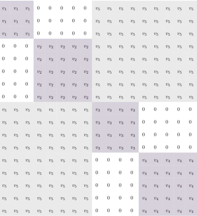
Let us consider a binary classification problem with both classes containing 2 subclasses. Let the first subclass of the first class contain 3 samples, and the second subclass 5 samples. Let the first subclass of the second class contain 4 samples and the second 5 samples. The structure of Lb can be observed from Tab. 3.1 and the structure of corre-sponding eigenvectors from (3.2), wherec corresponds to the class label,zto subclass label andri toi’thrandom value.

We can see that the matrix consists of blocks, where each diagonal block corresponds to instances of a certain class. In Tab. 3.1, different blocks are highlighted with different colors for the sake of clarity, and v1, v2, v3, and v4 are positive constant values

corre-sponding to the instances within the first and second subclass of the first and second class, respectively. v5 is a constant negative value, showing the relations between

in-stances of different classes.

Within each of the class blocks, a block structure showing the subclass structure of a class can be seen: the blocks corresponding to the instances of the same subclass have positive constant values, while the values corresponding to instances of different subclasses of the same class are zeros. The values corresponding to different classes are negative constant values. For data ofCclasses andZ subclasses in each class, the rank ofLb is equal toC∗Z−1, the matrix has the same amount of nonzero eigenvalues. The specific block structure ofLb dictates the specific structure of its eigenvectors:C−1 eigenvectors corresponding to the largest eigenvalues show the structure, from which the class label of each instance can be inferred, and the values at positions of the same class share the same value, and the values between classes are different. The rest of the eigenvectors show the subclass structure, where each eigenvector is responsible

(36)

Table 3.1. Structure of the between-class Laplacian matrix in SDA. v1 v1 v1 0 0 0 0 0 v5 v5 v5 v5 v5 v5 v5 v5 v5 v1 v1 v1 0 0 0 0 0 v5 v5 v5 v5 v5 v5 v5 v5 v5 v1 v1 v1 0 0 0 0 0 v5 v5 v5 v5 v5 v5 v5 v5 v5 0 0 0 v2 v2 v2 v2 v2 v5 v5 v5 v5 v5 v5 v5 v5 v5 0 0 0 v2 v2 v2 v2 v2 v5 v5 v5 v5 v5 v5 v5 v5 v5 0 0 0 v2 v2 v2 v2 v2 v5 v5 v5 v5 v5 v5 v5 v5 v5 0 0 0 v2 v2 v2 v2 v2 v5 v5 v5 v5 v5 v5 v5 v5 v5 0 0 0 v2 v2 v2 v2 v2 v5 v5 v5 v5 v5 v5 v5 v5 v5 v5 v5 v5 v5 v5 v5 v5 v5 v3 v3 v3 v3 0 0 0 0 0 v5 v5 v5 v5 v5 v5 v5 v5 v3 v3 v3 v3 0 0 0 0 0 v5 v5 v5 v5 v5 v5 v5 v5 v3 v3 v3 v3 0 0 0 0 0 v5 v5 v5 v5 v5 v5 v5 v5 v3 v3 v3 v3 0 0 0 0 0 v5 v5 v5 v5 v5 v5 v5 v5 0 0 0 0 v4 v4 v4 v4 v4 v5 v5 v5 v5 v5 v5 v5 v5 0 0 0 0 v4 v4 v4 v4 v4 v5 v5 v5 v5 v5 v5 v5 v5 0 0 0 0 v4 v4 v4 v4 v4 v5 v5 v5 v5 v5 v5 v5 v5 0 0 0 0 v4 v4 v4 v4 v4 v5 v5 v5 v5 v5 v5 v5 v5 0 0 0 0 v4 v4 v4 v4 v4

for a certain class. In this eigenvector, the values corresponding to instances of the same subclass of that class share the same value, while the values are different between subclasses and the values at the positions corresponding to other classes are 0.

Moreover, we can observe that eigenvectors showing the subclass structure of classes with a smaller number of instances correspond to bigger eigenvalues, and in the cases where multiple classes have an equal number of instances, eigenvectors that correspond to these classes merge. This means that in such eigenvectors structure of both classes can be observed, and the values corresponding to the other classes are zero. Such eigenvectors are repeated the number of times equal to the number of classes that have the same amount of elements.

(37)

In addition, we can observe that Lb is a constant sum block matrix [21], meaning that each of its rows and columns sums up to the same constant value. Being a constant sum block matrix,Lbis guaranteed to have a vector of ones as its eigenvector corresponding to eigenvalue 0 [21]. In addition, we can observe that for the data with a subclass structure, the eigenvectors maximizing the criterion (2.46) are those with the block structure as described. ⎛ ⎜ ⎜ ⎜ ⎜ ⎜ ⎜ ⎜ ⎜ ⎜ ⎜ ⎜ ⎜ ⎜ ⎜ ⎜ ⎜ ⎜ ⎜ ⎜ ⎜ ⎜ ⎜ ⎜ ⎜ ⎜ ⎜ ⎜ ⎜ ⎜ ⎜ ⎜ ⎜ ⎜ ⎜ ⎜ ⎜ ⎜ ⎜ ⎜ ⎜ ⎜ ⎜ ⎜ ⎜ ⎜ ⎜ ⎜ ⎜ ⎜ ⎜ ⎜ ⎜ ⎜ ⎜ ⎜ ⎜ ⎜ ⎝ ⎞ ⎟ ⎟ ⎟ ⎟ ⎟ ⎟ ⎟ ⎟ ⎟ ⎟ ⎟ ⎟ ⎟ ⎟ ⎟ ⎟ ⎟ ⎟ ⎟ ⎟ ⎟ ⎟ ⎟ ⎟ ⎟ ⎟ ⎟ ⎟ ⎟ ⎟ ⎟ ⎟ ⎟ ⎟ ⎟ ⎟ ⎟ ⎟ ⎟ ⎟ ⎟ ⎟ ⎟ ⎟ ⎟ ⎟ ⎟ ⎟ ⎟ ⎟ ⎟ ⎟ ⎟ ⎟ ⎟ ⎟ ⎟ ⎠ r1 r3 0 c= 1, z= 1 r1 r3 0 c= 1, z= 1 r1 r3 0 c= 1, z= 1 r1 r4 0 c= 1, z= 2 r1 r4 0 c= 1, z= 2 r1 r4 0 c= 1, z= 2 r1 r4 0 c= 1, z= 2 r1 r4 0 c= 1, z= 2 r2 0 r5 c= 2, z= 1 r2 0 r5 c= 2, z= 1 r2 0 r5 c= 2, z= 1 r2 0 r5 c= 2, z= 1 r2 0 r6 c= 2, z= 2 r2 0 r6 c= 2, z= 2 r2 0 r6 c= 2, z= 2 r2 0 r6 c= 2, z= 2 r2 0 r6 c= 2, z= 2 . (3.2)

Due to the described properties ofLb, its eigendecomposition can be avoided and substi-tuted with a much faster process: first, we select a vector of ones as its first eigenvector and then create Z∗C−1 eigenvectors of random values following the structure as de-scribed earlier, and orthogonalize them following the Gram-Shmidt process [22]. In the end, we remove the vector of ones since it is useless as it maps data instances to the same points. The process is described in detail in Algorithm 1.

(38)

Algorithm 1:Target vectors calculation, single-view case

FunctiongetSingleviewTargets(class_labels,cluster_labels,C,Z,N): Input: class_labels:N×1vector with class labels;

cluster_labels:N×1vector with the cluster labels;

Z :number of clusters in each class;

C:number of classes;

N :number of elements; %class-level vectors;

T ←N ×(C−1)matrix with random values at positions of different classes, such that values are repeated within the class in one column, but distinct between classes and columns;

L←unique numbers of elements in each class sorted in ascending order; %cluster level vectors;

forl←iterate throughLdo

k←list of classes withlelements;

m←length(k);

T clust←N ×m∗(Z−1)matrix with random values at positions of all

subclasses of classes ink, such that the values are shared within the subclass in one column, but distinct between subclasses and columns. Values at

positions of other classes are 0s;

T ←appendT clustas columns on the right; end

T ←appendN×1vector of ones as a column on the left; OrthogonalizeT;

remove the first column ofT; returnT

(39)

3.3 Multi-view Subclass Discriminant Analysis

As mentioned in the previous chapter, machine learning methods can take advantage of projecting multi-view data to some latent space and performing further analysis there. However, data within each view can be multi-modal as well, while most of the proposed methods rely on the assumption of its unimodality. To address this issue, a multi-view ex-tension to Subclass Discriminant Analysis, the Multiview Subclass Discriminant Analysis (MvSDA), is proposed.

We seek to find a projection space, projection onto which would result in different classes being far from each other while keeping all data samples close to each other. To achieve this, we maximize the distance between the means of subclasses of different classes, while minimizing the total scatter of the mean-centered data. The total scatter is therefore defined as St= V ∑ i=1 N ∑ k=1 yi_kyi_kT =YYT =WTXXTW, (3.3)

where yi_k is the k’th sample of view i in the latent space. The between-class scatter matrix is defined as Sb = V ∑ i=1 V ∑ j=1 C ∑ p=1 C ∑ q=1 q̸=p dp ∑ l=1 dq ∑ h=1 pi_plpj_qh(µi_pl−µj_qh)(µi_pl−µj_qh)T = V ∑ i=1 V ∑ j=1 WT_i XiLmv_bijXT_jWj =WTXLmv_b XTW, (3.4) X= ⎛ ⎜ ⎜ ⎜ ⎜ ⎜ ⎝ X1 0 ... 0 0 X2 ... 0 0 0 ... XV ⎞ ⎟ ⎟ ⎟ ⎟ ⎟ ⎠ , (3.5) W= ⎛ ⎜ ⎜ ⎜ ⎜ ⎜ ⎜ ⎜ ⎜ ⎜ ⎝ W1 W2 ... WV ⎞ ⎟ ⎟ ⎟ ⎟ ⎟ ⎟ ⎟ ⎟ ⎟ ⎠ , (3.6)

(40)

Lmv_b = ⎛ ⎜ ⎜ ⎜ ⎜ ⎜ ⎜ ⎜ ⎜ ⎜ ⎝ Lmv_b₁₁ Lmv_b₂₁ ... Lmv_bV₁ Lmv_b₁₂ Lmv_b₂₂ ... Lmv_bV₂ ... ... ... ... Lmv_b₁_V Lmv_b₂_V ... Lmv_{bV V} ⎞ ⎟ ⎟ ⎟ ⎟ ⎟ ⎟ ⎟ ⎟ ⎟ ⎠ , (3.7) Lmvbij = ⎧ ⎪ ⎪ ⎨ ⎪ ⎪ ⎩ 2∑C p=1 ∑C q=1 q̸=p ∑dp l=1 ∑dq h=1 V N_qhj Ni plN2 ei pleipl T − 1 N2eiple j qh T , ifi=j −2∑C p=1 ∑C q=1 q̸=p ∑dp l=1 ∑dq h=1 1 N2e i ple j qh T , otherwise , (3.8)

whereiandjare view labels,pandq are class labels,landhare subclass labels,pi_pl= Ni

pl

N is the prior of the subclasslof classpin the viewi,µ i

pl is the mean of the subclassl of classpin view i,ei

pl is the vector of lengthN with ones at positions corresponding to subclasslof classpin viewiand zeros elsewhere.

The optimal projection space is then obtained by optimizing the Fisher-Rao’s criterion:

J(W) = argmax

WT

iWi=I,i=1,...,V

T r(WTXLbXTW)

T r(WT_XXT_W) , (3.9)

whereXandWare defined as in (3.5) and (3.6), respectively, andKis centered. Equiv-alently, solution to the kernel version of the method is obtained by optimizing

J(A) =argmax

AT_KA₌_I

T r(ATKLbKTA)

T r(AT_KKT_A) , (3.10)

whereKis a block-diagonal matrix havingKv as itsv’thblock:

K= ⎛ ⎜ ⎜ ⎜ ⎜ ⎜ ⎝ K1 0 ... 0 0 K2 ... 0 0 0 ... KV ⎞ ⎟ ⎟ ⎟ ⎟ ⎟ ⎠ (3.11)

The solution to (3.9) is obtained by solving the eigendecomposition problemLbXTv =

λXTv. Similarly, the solution to (3.10) is given by LbKa = λKa. The solution can be obtained following Spectral Regression similarly to the process described in section 3.1.