Statistical Methods for Networks with Node Covariates

(1)

Statistical Methods for Networks with Node

Covariates

by Yumu Liu

A dissertation submitted in partial fulfillment of the requirements for the degree of

Doctor of Philosophy (Statistics)

in The University of Michigan 2020

Doctoral Committee:

Professor Ji Zhu, Chair

Assistant Professor Yang Chen Assistant Professor Walter Dempsey Professor Elizaveta Levina

(2)

Yumu Liu liuyumu@umich.edu ORCID ID: 0000-0001-5108-1654

c

(3)

ACKNOWLEDGEMENTS

I would like to express my greatest appreciation to my advisor Professor Ji Zhu for his kindness and providing helpful advice and discussions on the research projects, and also for his endless support and encouragement outside academic during my PhD study. I am also very grateful to Professor Elizaveta Levina, who has provided a lot of helpful advice and guidance as a close member of the research group. Further, I would like to thank Professor Yang Chen and Professor Walter Dempsey for serving as my committee member and providing insightful suggestions. Last but not least, many thanks should be attributed to my parents who provided me this opportunity to start this journey and continuously provided me with their support and encour-agement both physically and mentally along these years.

Five years ago, I was entering a vast forest in the field of science. I stood in awe before the lush green tree of statistics. I was driven to explore it in hopes of making a discovery. The various forms and amazing colors of even the smallest leaves have inspired me to pursuit my study. I am fortunate to be a part of the family of the De-partment of Statistics at the University of Michigan, the time here will be a precious and memorable part of my life.

(4)

LIST OF FIGURES

Figure

2.1 Graphical Representation of the Model . . . 11

2.2 Mean accuracy vs r for K = 2, β∼U(−1,1) . . . 26

2.3 Mean accuracy vs r for K = 2 . . . 27

2.4 Mean accuracy vs r for K = 5, β ∼U(−1,1) . . . 28

2.5 Mean accuracy of clustering vs r for K = 5 . . . 29

2.6 Mean accuracy vs r for K = 2 with misspecified covariates . . . 29

2.7 Mean balanced accuracy vs r for K = 2 with unbalanced communi-ties, pkk=0.15,β = 1 . . . 30

2.8 Mean accuracy vsr forK = 2 with non-assortative networks, initial-ized with CASC, pk`=0.15 . . . 31

2.9 Degree distribution . . . 33

2.10 Community detection result . . . 34

3.1 Imputation results for continuous variable . . . 55

3.2 Imputation results for binary variables . . . 56

3.3 Imputation results for continuous variables when network is irrelavent 57 4.1 log(nnodes) vs log(nedges) . . . 71

4.2 log(proportion) vs log(degree) . . . 73

4.3 Full Enron email network, log(nnodes) vs log(degreetotal) . . . 75

(7)

LIST OF TABLES

Table

2.1 Mean computation time of community detection algorithms under

degree corrected blockmodels with covariates over 10 replications . . 32

3.1 Summary of the PIRA network . . . 59

3.2 AuROC of the imputation on the PIRA data set . . . 59

4.1 Estimate when trueα = 0.5,θ = 10 . . . 74

4.2 Estimate when trueα = 0.3,θ = 10 . . . 74

4.3 Estimates for Enron network, T:Trader, M: Manager, D: Director, VP/P: Vice President/President . . . 77

C.1 Estimation when true α= 0.7, θ = 10 . . . 108

(8)

LIST OF APPENDICES

Appendix

A. Appendix for Chapter II . . . 79 B. Appendix for Chapter III . . . 96 C. Appendix for Chapter IV . . . 103

(9)

ABSTRACT

Network data, which represent relations or interactions between individual entities, together with nodal covariates information, arise in many scientific and engineering fields such as biology and social science. This dissertation focuses on developing sta-tistical models and theory that utilize information from both the network structure and node covariates to improve statistical learning tasks, such as community detec-tion and missing value imputadetec-tion.

The first project studies the problem of community detection for degree-heterogeneous networks with covariates, where we aim to cluster the nodes into groups that share similar patterns in link connectivity and/or covariates distribution. We consider in-corporating node covariates via a flexible degree-corrected block model by allowing the community memberships to depend on node covariates, while the link probabil-ities are determined by both node community memberships and degree parameters. We develop two algorithms, one using the variational inference and the other based on the pseudo-likelihood for estimating the proposed model. Simulation studies indicate that the proposed model can obtain better community detection results compared to methods that only utilize the network information. Further, we show that under mild conditions, the community memberships and the covariate parameters can be estimated consistently.

The second project considers the problem of missing value imputation when indi-viduals are linked through a network. We assume the edges in the network are

(10)

related with the distances in the covariates of the individuals through a latent space network model. We propose an iterative imputation algorithm that is flexible and utilizes both the correlation among node variables and the connectivity between ob-servations given by the network. We relate the proposed method to a Bayesian model and discuss the convergence of the imputation distribution when the specified condi-tional models for imputation are compatible with the true underlying model of the covariates. We also use simulation studies and a data example to illustrate empirically that the imputation accuracy can be improved by incorporating network information.

The final contribution of this dissertation is on incorporating covariates under the edge exchangeable framework. Edge exchangeable models have attractive theoretical and practical properties which make them appropriate for modeling many sparse real-world interaction networks constructed through edge sampling mechanisms. However, as far as we know, there is no edge exchangeable network model that allows for node covariates. In the third project, we propose a model that incorporates node covariates under the edge exchangeable model framework and show that it enjoys properties such as sparsity, and partial exchangeability. We further develop a maximum likelihood es-timation method to estimate the model parameters and demonstrate its performance through both simulation studies and a data example.

(11)

CHAPTER I

Introduction

Network data arise naturally in many areas nowadays due to the advances in technol-ogy. In these network data, researchers use edges to represent relations or interactions between entities represented by nodes. Examples include but not limited to social networks where nodes are individual persons and edges are relations like friendships, biological networks where nodes are proteins and edges are their interactions, and etc (Karrer and Newman, 2011). Many works in the past decades have built up various tools for analyzing the structures or the development of the networks and have dif-ferent focuses.

On analyzing the structure of a network, community detection is one of the most important questions that was widely studied. Community detection aims to cluster the nodes in the networks into communities with similar connectivity patterns (For-tunato, 2010). The study of community structures in network can be dated back to Zachary (1977) with empirical observations that real-world networks typically showed a pattern that nodes form groups with more connections within the same group than between groups. Many statistical models have been established to understand and uncover the community structure, among which the stochastic blockmodel (Holland et al., 1983) and its extensions, including the mixed membership stochastic

(12)

blockmod-els (Airoldi et al., 2008) and the degree corrected stochastic blockmodblockmod-els (Karrer and Newman, 2011) are the most popular ones. Model free methods based on modularity criteria (Newman, 2006), spectral methods (Rohe et al., 2011; Qin and Rohe, 2013; White and Smyth, 2005), and other methods (Veldt et al., 2018; Zhao et al., 2011; Wang et al., 2011; Amini and Levina, 2014) are also available. Theoretical guaran-tees of community detection has also been established for various models based on stochastic blockmodels and various methods (Zhao et al., 2012; Bickel et al., 2013; Celisse et al., 2012;Lei et al., 2015). Another set of literature that focus on explaining the network structure assume that the nodes of the networks live in a low dimensional euclidean space. This includes the latent space models (Hoff et al., 2002;Hoff, 2005), and the random dot product graph model (Young and Scheinerman, 2007). These models have the potential to explain some higher order characteristics in networks like abundance of triangles, which is not captured in stochastic blockmodels (Hoff, 2005). And the random dot product graph shows nice limiting properties (Athreya et al., 2016). More details of the models can be seen in the survey paper by Athreya et al. (2017).

Other than focusing on the structure of a snapshot of the network, researchers also showed interests in understanding the mechanisms for how the networks are evolved over time, and also in explaining some commonly observed characteristics in real-world networks. Specifically, the sparse network phenomenon and the power-law degree distribution are of attention (Barab´asi and Albert, 1999; Leskovec et al., 2008). The sparse network and power-law degree distributions are related to the study of preferential attachment models (Newman, 2001; Wan et al., 2017; V´azquez, 2003; Jeong et al., 2003), and are important factors that initiates the study of edge-exchangeable models (Crane and Dempsey, 2018;Cai et al., 2016). On the exchange-ability structure of network models, most of the literature have been focusing on node

(13)

exchangeable models including random dot product graph (Young and Scheinerman, 2007), stochastic blockmodels (Holland et al., 1983), and graphon models (Wolfe and Olhede, 2013; Choi et al., 2014). The edge changeable framework developed inCrane and Dempsey (2018);Cai et al.(2016) has been attracting the attention of researcher due to its nice limiting properties mentioned above and interpretation in terms of sampling. Specifically, edge exchangeable framework is natural in the case where the network data is collected by directly sampling edges instead of sampling the nodes.

Along with the network, often the traditional covariates information are also col-lected on each node, such as the characteristics of each person in a social network (Leskovec and Mcauley, 2012;Van de Bunt et al., 1999). These covariates may contain information that are related to the network structures. For example, the nodes that are connected in a social network may have similar covariates, which is known as the homophily phenomenon (McPherson et al., 2001;Fujimoto and Valente, 2012; Chris-takis and Fowler, 2007). Thus, such information can be very helpful in understanding the network structures of interest. Some models and methods that incorporate the covariates information to assist community detection have been developed in the lit-erature, see for example (Newman and Clauset, 2016; Xu et al., 2012; Yang et al., 2013; Binkiewicz et al., 2014; Weng and Feng, 2016). In more traditional multivari-ate analysis, the covarimultivari-ates themselves can be of interests. In that case, the network information may be helpful to improve the analysis to the covariates. Only a handful of literature considered such setting and focused on prediction (Asur and Huberman, 2010; Wolf et al., 2009;Li et al., 2019). In social science studies, methods have been proposed to make inference on causal effects with network interference (Shalizi and Thomas, 2011;Manski, 2013;Kao, 2017;Basse and Airoldi, 2015). In machine learn-ing literature, heuristics like label propagation algorithms (Zhur and Ghahramanirh, 2002) have been developed for classifying nodes on a network with a part of the node

(14)

labels observed, which can be viewed as imputation for a single categorical variable utilizing network information.

This dissertation aims to develop models and statistical procedures that incorporate both network and node covariates information to improve the performance in com-munity detection, missing value imputation, and in enriching the edge exchangeable models. For all the three targets, we view the observed network as a random object generated from some underlying distributions or mechanisms. The distribution of the covariates may or may not be considered random depending on specific applications.

The rest of the thesis is organized as follows:

Chapter II focuses on improving community detection by utilizing covariates in de-gree heterogeneous networks. Specifically, we proposed a model that combines the degree-corrected stochastic blockmodel and models for multivariate classification or clustering. We developed two algorithms for estimating the model based on varia-tional inference or pseudo likelihood method. We established consistency results for the pseudo likelihood algorithm and illustrated that the community detection result was improved with covariates information incorporated.

Chapter III focuses on improving multivariate missing value imputation by incorpo-rating network information. We assumed that the probability of two nodes connecting with each other in the network is correlated to the distance between the covariates of the two node through a latent space model. We considered combining the flexible iterative imputation with chained equation framework with the network model and developed gradient based methods for making imputations. We discussed the con-nection between the iterative imputation with chained equation framework and the

(15)

Gibbs sampling and Bayesian models.

Chapter IV extends the Hollywood model, a canonical edge exchangeable model to incorporate node covariates. The main difficult of incorporating covariates into edge exchangeable models is that the exchangeability structure can be broken easily. We address the question that to what extent we can preserve the edge exchangeability and what it means from a sampling perspective. We developed an estimation algo-rithm for the model and illustrated the model using simulation and Enron email data. We also showed that the proposed model inherits the sparsity property in limit.

(16)

CHAPTER II

Network Community Detection via the

Degree-corrected Block Model with Node

Covariates

2.1 Introduction

A commonly asked question when studying a network is that “can we identify groups of nodes that share similar connectivity patterns”, which leads to the community de-tection problem, one of the fundamental problems in network analysis. Many methods have been proposed and studied, and they can be mainly divided into two categories: (1) model-free methods that do not try to fit a generative probabilistic model, and (2) model-based approaches using probabilistic network models. Notice that the two categories are not totally divided, many model-free methods also exhibit good per-formance under commonly used probabilistic network models.

In the model-free regime, different methods have been considered for community detection. For example, Newman (2006) proposed modularity as a criterion repre-senting the “strength” of a community assignment and transformed the community detection problem to optimization of a certain criterion. Another approach to the problem is by exploring spectral properties of the adjacency matrix or the

(17)

corre-sponding Laplacian matrix. Literature including Jin (2015); Qin and Rohe (2013); Rohe et al.(2011) have developed various spectral clustering algorithms and analyzed their performances.

In model-based approaches, the stochastic blockmodel (Holland et al., 1983) is prob-ably the most commonly used model. For a network withn nodes, given node labels ci ∈1,2, ..., K, the probability of having an edge between nodei and j is

P(Aij = 1|ci, cj) =Bcicj ,

where {Bab} is a K×K parameter matrix. The model intuitively explains the

com-munity structure that nodes within the same group share similar link patterns. Ex-tensions such as the mixed membership models (Airoldi et al., 2008) and the degree-corrected blockmodel (Karrer and Newman, 2011) have been proposed to accommo-date different real network properties. Specifically, the degree-corrected blockmodel assumes that there is a degree parameterθiassociating with nodei, andAij is Poisson

distributed with

E(Aij|ci, cj) =θiθjBcicj .

This allows for degree heterogeneity even within the same community, which makes the model much more flexible and works better in many real-world networks. Another important family of the network models is the latent space model that is studied by literature including Hoff (2005),Hoff et al. (2002). The latent space model assumes that each node has a latent position in some euclidean space and the probability of forming an edge between two nodes depends on some form of distance between their latent positions.

(18)

over all possible community label assignments. Estimation using MCMC under the Bayesian framework has been developed in the early stage (Nowicki and Snijders, 2001) and methods based on variational inference have been developed and studied to make the computation tractable recently (Airoldi et al., 2008; Bickel et al., 2013; Celisse et al., 2012). Another way of fitting blockmodels is by the profile likelihood (Bickel and Chen, 2009;Zhao et al., 2012), which establishes criteria that only depend on the label assignments by profiling out parameters for any fixed label assignments. Blockmodels are then fitted by optimizing these criteria via greedy algorithms. Re-cently, Amini and Levina (2014) proposed semi-definite relaxation that transforms the problem into an optimization where the argument is a semi-definite matrix by relaxing some constraints in the maximum likelihood problem. Last but not least, Amini et al. (2013) proposed a fast pseudo likelihood algorithm that scales well to large networks for both the stochastic blockmodel and the degree corrected extension by neglecting the dependence resulting from symmetry in undirected network.

For the community detection problem, the main theorectical interest lies in studying the consistency of estimated community label assignments. A commonly used notion of consistency is given inBickel and Chen (2009) and Zhao et al.(2012):

strong consistency: P(ˆc=c)→1, as n→ ∞ weak consistency: P(1 n n X i=1 1(ˆc6=c)< )→1, for any as n→ ∞

Strong consistency of the clustering result has been established in general for profile likelihood based methods under the stochastic blockmodel family and its extension (Bickel and Chen, 2009; Bickel et al., 2015; Zhao et al., 2012) when the average de-gree of the graph is growing fast enough. Specifically, the average dede-gree needs to grow faster than logn. The consistency of variational inference under the

(19)

stochas-tic blockmodel has been obtained in Mariadassou and Matias (2015); Celisse et al. (2012). With mild assumptions on the initialization, pseudo likelihood method has been shown to be weakly consistent (Amini et al., 2013). Spectral methods have also been shown to have similar theoretical guarantees (Jin, 2015; Lei et al., 2015; Qin and Rohe, 2013; Rohe et al., 2011). On top of the studies on consistency of cluster-ing, asymptotic theories regarding the parameter estimates have also been established under the stochastic blockmodel for methods based on maximum likelihood (Celisse et al., 2012) or its approximation via variational inference (Bickel et al., 2013).

The work mentioned above focus on utilizing the network information alone. However, in real applications, especially in social networks, the structured network data col-lected using modern technologies often contain additional information on the nodes, or node covariates, about the individuals in the network. In many cases, it is natural to believe that these node covariates can be helpful in refining the communities that are given only using the network information in terms of both accuracy and inter-pretation. For example, in social networks, two people with similar background may have a higher probability to be connected.

Several methods have been developed to incorporate the node covariates into the community detection procedures. For examples, Binkiewicz et al.(2014) proposed a variant of spectral clustering by using the weighted sum of the graph laplacian and the gram matrix as input; Yan and Sarkar(2016) extended the semi-definite relaxation by adding in a k-means type penalty to the objective function; Zhang et al.(2015) proposed a joint community detection criterion representing the community strength together with node covariates similarities. Weng and Feng(2016) and Newman and Clauset(2016) have also considered to extend the stochastic blockmodel or the degree-corrected blockmodel to incorporate node covariates. However,Weng and Feng(2016) focuses only on the stochastic blockmodel, whileNewman and Clauset(2016) can only

(20)

allow one categorical covariate.

In consideration of the flexibility, in this chapter, we propose a model that natu-rally combines the degree-corrected stochastic blockmodel and the classical logistic regression for the community detection problem. We choose the degree-corrected blockmodel to model the network as it is not only flexible theoretically, but also has been proven to perform well in fitting many real-world networks. We choose to use the multinomial logistic regression to model the relation between covariates and com-munity labels as it does not make many assumptions on the distribution of covariates and is thus flexible. It is also possible to use mixture models, which might be helpful if we have prior knowledge about the distribution of the covariates. In section 2.3, we develop a variational EM algorithm and a pseudo likelihood algorithm for its estima-tion and study asymptotic properties for the pseudo likelihood algorithm in Secestima-tion 2.4. We further illustrate their performances under various simulation settings and on a data example in Sections 2.5 and 2.6 respectively.

2.2 Model

Suppose we observe an undirected network of n nodes with self-loop and multi-edges allowed. We represents the network by an symmetric adjacency matrix A = {Aij}, i, j = 1,2..., n, whose diagonal elementAiiis equal to twice the number of edges

from node ito itself. An n×p covariate matrix X ={Xij}, i= 1,2..., n, j = 1,2..., p

is also observed. Besides, there is an unobserved community membership matrix C = {Cik}, i = 1,2..., n, k = 1,2..., K where K is the total number of communities,

and Cik = 1 if node iis in community k. We use ci to denote the community label of

nodei, i.e. ci =k if node i is in community k.

(21)

de-A X

C

Figure 2.1: Graphical Representation of the Model

pendence structure between A, X and C. The joint probability of this model would be P(A, X, C) = P(X)P(C|X)P(A|X, C). We do not model P(X) as it does not involve C and instead, we work withP(C, A|X) =P(A|X, C)P(C|X).

Given node covariates X and community membership C, we assume the network A|X, C is generated from the Degree-Corrected Stochastic Blockmodel (DCBM)(Karrer and Newman, 2011). Then the networkA is dependent onX implicitly through a set of latent degree correction parametersθ ={θi}, i= 1,2, ..., n, which is represented by

the dashed line in the graphical representation. Conditional on the node labels, the number of edges between a node pair (i, j) is Poisson distributed with meanθiθjBcicj,

independent of any other node pairs, where B ={Brs}, r, s = 1,2..., K, is a K×K

matrix determining the propensity of forming edges between nodes from community r and s. Since the network is undirected, B should be symmetric. Following this setting of DCBM we will have

P(A|X, C;θ, B) =Y i<j (θiθjBcicj) Aij Aij! exp(−θiθjBcicj) ×Y i (1₂θ_i2Bcicj) Aii/2 (Aii/2)! exp(1 2θ 2 iBcicj) =Y i<j K Y k,l=1 (θiθjBkl)AijCikCjl (Aij!)CikCjl exp(−θiθjBklCikCjl) ×Y i K Y k=1 (1₂θ2 iBkk)AiiCik/2 ((Aii/2)!)Cik exp(−1 2θ 2 iBkkCik) . (2.1)

(22)

We model P(C|X) using a multinomial logistic regression model with parameter β = {βk}, k = 1,2, ...K. For identifiability, βK is set to 0. Here we use a compact

notation by implicitly including the intercept into β and let the covariates matrixX have a corresponding dummy column of 1,

P(C|X, β) = n Y i=1 exp(βcixi) PK k=1eβkxi = n Y i=1 K Y k=1 (exp(βkxi) PK l=1eβlxi )Cik _. (2.2)

2.3 Estimation

In this section, we develop a variational EM algorithm and a pseudo likelihood algo-rithm to estimate the model described in the previous section.

2.3.1 Variational EM algorithm

Since the community membershipC is unknown, we can use the EM algorithm with C being the latent variable to find the maximum likelihood estimate of the parame-ters Θ ={B, β, θ}. As an intermediate step of EM algorithm, the estimation of the conditional distributionP(C|A, X) is also calculated.

For the likelihood P(A|X,Θ) we have

logP(A|X; Θ) ≥logP(A|X,Θ)−DKL(R(C|A, X)||P(C|A, X,Θ))

= Z

C

R(C|A, X)[logP(A, C|X,Θ)−logR(C|A, X)]

:= Z C R(C|A, X)l(Θ|C) :=L(R,Θ) , (2.3)

(23)

whereR(C|A, X) is any conditional distribution ofC givenA, X. EM algorithm tries to maximize L by alternately maximizing Lover R and Θ, which gives

E-step: given Θ(t)_{, take}_R(t+1)₌_P_{(C|A, X,}_Θ(t)_{) and compute}

l(Θ|Θ(t)) =X C P(C|A, X,Θ(t))l(Θ|C) M-step: compute Θ(t+1) = arg max Θ l(Θ|Θ (t)_{) .}

In practice, however, there are Kn configurations of C and P(C|A, X,Θ(t)) cannot be factorized, which makes the E-step computationally intractable. To handle this difficulty, we use the variational approximation (Jordan et al., 1999) which considers a restricted family of the conditional probabilityP(C|A, X). Specifically, we consider R(C|A, X) = Qn

i=1

QK

k=1τ

Cik

ik , where τ is a set of variational parameters. With this

choice of R(C|A, X), we make the restriction that Ci, i = 1,2, ..., n are independent

given A, X and follows a multinomial distribution with K-dimensional probability vector τi·.

(24)

The objective function to maximize now becomes

J(τ,Θ) :=X

C

R(C|A, X)[logP(A, C|X,Θ)−logR(C|A, X)]

=E[logP(A, C|X,Θ)−logR(C|A, X)]

=X i<j K X k,l=1 τikτjl[Aijlog(θiθjBkl)−log(Aij!)−θiθjBkl] + n X i=1 K X k=1 τik[ Aii 2 log( 1 2θ 2 iBkk)−log(( Aii 2 )!)− 1 2θ 2 iBkk] + n X i=1 K X k=1 τik[βkxi−log( K X k=1 eβkxi_)]₋ n X i=1 K X k=1 τiklog(τik) . (2.4)

The maximization problem can then be solved using an EM-like algorithm with: E-step: τ(t+1) = arg maxJ(τ,Θ(t))

M-step: Θ(t+1) _{= arg max}_J_(τ(t+1)_,_{Θ) .}

2.3.1.1 E-step

The E-step is to maximize J(τ,Θ) with respect to τ for given Θ; this can be solved by fixed point iteration. For i= 1,2, .., n

τik ∝( 1 2θ 2 iBkk) Aii 2 exp(β_kx_i− 1 2θ 2 iBkk) × n Y j=1,j6=i K Y l=1 [(θiθjBkl) Aij (Aij!) exp(−θiθjBkl)]τjl (2.5)

for k = 1,2, ..., K and subject to PK

(25)

2.3.1.2 M-step

The M-step is to maximize J(τ,Θ) with respect to Θ for givenτ; this can be divided into two sub-problems that optimize with respect to (θ, B) and β respectively. For (θ, B), the objective function is

g(θ, B) = X i<j K X k,l=1 τikτjl[Aijlog(θiθjBkl)−θiθjBkl] + n X i=1 K X k=1 τik[ Aii 2 log( 1 2θ 2 iBkk)− 1 2θ 2 iBkk] , (2.6)

with the constraints Bij = Bji for undirected network, and θi > 0 by definition.

The parameters θ are only identifiable within a multiplicative constant that will be absorbed into B, so we also need the constraint Pn

i=1θi = 1 for identifiability. To

compute the maximizers, we set the gradient to 0 and iteratively solve the equation system. The objective function is concave with respect to each θi and the update for

θi with all other variables fixed has analytical solutions as follows:

ˆ θi = −b−√b2₋_4ac 2a a=− K X k=1 Bkkτik b=−X j6=i K X k,l=1 θjBklτikτjl c=X j6=i K X k,l=1 Aijτikτjl+ K X k=1 Aiiτik . (2.7)

θi are normalized to have sum equal to 1 to satisfy the identifiability constraint after

each iteration of updates. In practice we run a fix number of iterations (2.7) to get a result close to convergence.

(26)

function is concave with respect to B. ˆ Bkl = P i<j[τikτjlAij +τilτjkAij] P i<j[τikτjlθiθj +τilτjkθiθj] , for k 6=l ˆ Bkk = P i<jτikτjkAij + P iτik Aii 2 P i<jτikτjkθiθj + P iτik θ2 i 2 . (2.8)

We then iterate (2.7) and (2.8) until convergence.

Maximizing J(τ,Θ) with respect to β is a multinomial logistic regression problem. For numerical stability we include a ridge penalty and maximize

L(β) = n X i=1 K X k=1 τik[βkxi−log( K X k=1 eβkxi_)]₋_λ||β||2 2 (2.9)

where λ >0 is a small positive number. This can be solved using existing packages, such as the glmnet package in R.

2.3.1.3 Initialization

The speed of convergence often depends on the initial values of the algorithm. We initialize the parameters by first initializing community labels using regularized spectral clustering(RSC) and initialize θi proportional to di, the degree of node i.

Note this requires the network to have no isolated node. Then we setτ to be a binary matrix corresponding to the initial community labels. With τ, θ initialized, B and β can be calculated using (2.8) and (2.9).

2.3.2 Pseudo likelihood based algorithm

As mentioned in the variational EM algorithm, the main challenge in maximizing the joint likelihood using EM algorithm lies in the E-step as it is intractable. The main

(27)

idea of pseudo likelihood is to simplify the likelihood and make it tractable by ignoring some of the dependency structure. Specifically for stochastic blockmodels, a pseudo likelihood can be established by ignoring the symmetry of the adjacency matrix. In this section, we first give an brief review on the pseudo likelihood method introduced inAmini et al. (2013) and then make modifications to involve node covariates.

2.3.2.1 Pseudo likelihood for blockmodel

Let the true community label be denoted by ci, i = 1,2, ..., K. Given an initial

labeling e = {ei}, i = 1,2, ..., n, ei ∈ 1,2, ..., K, we will work with the following

quantity,

bik =

X

j

Aij1(ej =k), i= 1, ..., n, j = 1, ..., K. (2.10)

Letbi = (bi1, bi2, ..., biK) and further let R be aK ×K matrix with

Rka= 1 n n X i=1 1(ei =k, ci =a)

and Rk· be the k-th row. Let B be the K×K parameter matrix for the blockmodel

and B·` be the `-th column of B. Let λ`k =nRk·B·` and Λ ={λ`k}.

The pseudo likelihood for a stochastic blockmodel is established based on the fol-lowing key observations: for each node i, given the true labels c with ci =`,

(A) {bi1, bi2, ..., biK} are mutually independent, and

(B) bik is approximately Poisson distributed with mean λ`k.

With true label ci unknown, bi is a mixture of Poisson vectors. Then by ignoring

the dependence betweenbi, i= 1,2, ..., n, we have the following pseudo log-likelihood

(up to a constant): lP L(π,Λ;{bi}) = n X i=1 log( K X `=1 [π`e−λ` K Y k=1 λbik `k]), (2.11)

(28)

where λ` =P_kλ`k and π` is the probability of a node being in community `.

2.3.2.2 Conditional pseudo likelihood for DCBM

Extending the pseudo likelihood to DCBM is non-trivial. The degree corrected model has n degree parameters, one for each node, which makes the pseudo likelihood and estimation much more complicated. Amini et al.(2013) proposed a simple alternative that considers the pseudo likelihood conditional on the observed node degrees. By conditioning on the observed node degrees, the degree parameters do not play a role in the pseudo likelihood anymore and we only need to focus on the block structures. The key observation in the conditional pseudo likelihood is that conditioning on the observed node degree di =

P

kbik and true community label ci = `, the variables

(bi1, bi2, ..., biK) are multinomially distributed with parameters (di;ψ`1, ψ`2, ..., ψ`K),

withψ`k = λ_λ`k

`. Then we have the conditional log pseudo likelihood (up to a constant):

lCP L(π,{ψlk};{bi}) = n X i=1 log( K X `=1 [π` K Y k=1 ψbik `k ]). (2.12)

2.3.2.3 Conditional pseudo likelihood for DCBM with node covariates

We now introduce the conditional pseudo likelihood with node covariates and develop a corresponding estimation algorithm.

Note that in our proposed model, the node covariates only affect the formation of the network through community probability. Thus, we replace π` by

exp(β`Xi)

P

kexp(βkXi),

which is the probability of node i being in community ` under the logistic regres-sion model. This gives us the following conditional log pseudo likelihood (up to a

(29)

constant): LCP L(β,{ψ`k};bi) = n X i=1 log( K X `=1 [ exp(β T ` xi) PK k=1exp(β T kxi) K Y k=1 ψbik `k ]). (2.13)

Then we can obtain the estimate ofβ,{ψ`k}by maximizing the conditional log pseudo

likelihood via the EM algorithm for mixture models. With the parameter estimate, we update the initial label e and repeat the procedure for T iterations.

Let nk(e) = P_i1(ei = k), nk`(e) = nk(e)nl(e), nkk(e) = nk(e)(nk(e) − 1) and

Ok`(e) = P_ijAij1(ei =k, ej =`). The algorithm consists of the following steps:

• Initialize label e using regularized spectral clustering, and initialize β corre-spondingly. Let ˆπ` =n`/n, let R =diag(ˆπ), ˆB`k =O`k/n`k, ˆλ`k =nRˆk·Bˆ·` and

initialize {ψ`k} by row normalization of Λ.

• Repeat T times:

– (1) compute block sumsbi under current{ei}, i= 1,2, ..., n

– (2) E-step: Given ˆβ,{ψˆ`k}, compute Pi`:=P(ci =`|bi, xi)

Pi` :=P(ci =`|bi, xi) = ˆ πi` QK m=1ψˆ bim `m PK k=1πˆik QK m=1ψˆ bim km (2.14) where ˆπi`= exp( ˆβT `xi) PK k=1exp( ˆβTkxi).

(30)

– (3) M-step: Given Pil, update β by logistic regression and update Θ ˆ ψ`k = Pn i=1Pi`bik Pn i=1Pi`di (2.15)

– (4) repeat (2) and (3) until the parameters converge

– (5) update labelei = arg maxlPi` and return to step (1) .

The algorithm typically only needs a few label updates until convergence, but the performance relies on suitable initial labels.

2.4 Theoretical properties

The main theoretical property that community detection methods pursue is consis-tency of the community estimates ˆc. A commonly used definition of consistency is fromBickel and Chen (2009) and Zhao et al.(2012):

strong consistency: P(ˆc=c)→1, as n→ ∞ weak consistency: P(1 n n X i=1 1(ˆc6=c)< )→1, for any as n→ ∞ .

Note that the consistency notion is up to label permutations. For example, switching the label of community 1 and community 2 does not change the community structure.

Although we have developed the algorithm with multi-edges allowed, we will study the theoretical property based on binary networks to simplify the problem. In most real applications, we only observe binary networks and care more about whether an edge is present or not rather the multiplicity of the edges, thus this simplification is

(31)

reasonable.

Methods based on maximum profile likelihood have been shown to be strongly con-sistent under both stochastic blockmodel and its degree-corrected extension (Zhao et al., 2012), but consistency of community label estimates under variational infer-ence is only established under stochastic blockmodel (Mariadassou and Matias, 2015; Weng and Feng, 2016), with indispensable dependence on the consistency result for estimating the K × K matrix parameter B that controls inter and intra commu-nity connectivity (Bickel et al., 2013; Celisse et al., 2012).However, extending these consistency results to variational inference under the degree-corrected blockmodel is challenging, since the consistency of the estimates for B cannot be easily obtained due to identifiability issues in the degree correction parameters. Nonetheless, the consistency of maximum profile likelihood still holds followingZhao et al. (2012) and the weak consistency result for pseudo likelihood algorithm similar to that in Amini et al. (2013) can be shown. We will focus on showing the consistency of the pseudo likelihood, based on the results from Amini et al.(2013).

For theoretical analysis of the pseudo likelihood algorithm, we only consider the case K = 2. Further, for simplicity, we assume that among the n nodes, m = n₂ nodes are in community 1 and assume the initial label e is also balanced, which means e

assignsm nodes to community 1 andm nodes to community 2. We will first consider a directed graph. For the directed graph, we will use ˜Aij to denote the adjacency

matrix and ˜B to denote the K×K matrix parameter. The directed graph model is actually natural for pseudo likelihood approach since it is the model where the row independence assumption holds. We let the edge probability matrix of the directed graph ˜B = _m1    a b b a  

(32)

The key assumption is that among the m nodes with initial labels being commu-nity 1, γm nodes are truly in community 1. It is not difficult to see that this also implies that the initial labels e also have γm correctly labeled nodes in community 2. We do not assume we know the value ofγ or which labels are matched. But we do assume γ ∈(0,1)\{1

2} and mγ is an integer. Let E

γ _{denote the collection of all such}

initial labeling Eγ ₌_Eγ n = ( e∈ {1,2}n _: m X i=1 1(ei = 1) =mγ = n X i=m+1 1(ei = 2) ) .

We will focus on the E-step of the pseudo likelihood algorithm. With some initial estimates ˆa,ˆb as well as ˆβ, together with initial labeling e, the labels are estimated by

ˆ

ci(e) = arg max k∈{1,2}{ ˆ βkXi+ 2 X m=1 ˜

bim(e) log ˆγkm(e)} , (2.16)

where ˆγkm are the elements of the row normalized matrix of ˜Λ = [nR(e) ˜B]T, with ˜B

estimated by plugging in ˆa,ˆb.

LetC(γ) := hlogψˆ11(e)

ˆ ψ21(e)

i−1

, and define the mismatch ratio

˜ Mn(e) := min φ∈{(1,2),(2,1)} 1 n n X i=1 1[ˆci(e)6=φ(ci)],

whereφ is considering the fact that the labels are identified up to a permutation. We will show a consistency result based on the convergence of this mismatch ratio, which corresponds to the weak consistency definition.

Let us consider the initial estimates (ˆa,ˆb) that have the same ordering as true param-eter (a, b) such that (ˆa−ˆb)(a−b)>0. We have the following result.

Theorem II.1. Under the balanced communities assumption, let γ ∈ (0,1)\{1 2}.

(33)

Let the adjacency matrix A˜ be generated under the directed graph model with edge-probability matrix B˜ and assume a6=b. In addition, assume |βXˆ i| ≤M, where M is

a constant, and

m:= (1−2γ)(a−b)− |M C(γ)| ≥0 (1−2γ)(a−b) +|M C(γ)| ≤3(a+b)

(2.17)

Then there exists a positive sequence {un} such that

logun+ log logun≥log(

4 e) +

m2

4(a+b)

and the mismatch ratio has

P sup σ∈Eγ ˜ Mn(e)> 4h(γ) logun ≤exp{−[h(γ)−κγ(n)]n} (2.18)

where h(p) =−plogp−(1−p) log(1−p)is the binary entropy function and κγ(n) := 1 n[log( n 4πγ(1−γ)) + 1 3n] =o(1).

In particular, if _4(a+b)m2 → ∞, we have un → ∞ and the pseudo likelihood estimate is

consistent.

Remark II.2. _4(a+b)m2 → ∞ implies (1−2γ)(a−b) → ∞ and the assumptions (2.17) are then satisfied for sufficiently large n, indifferent of the value of γ. The condition

m2

4(a+b) → ∞ itself is also not strong if we assume γ fixed. For example, if we let

a= logn and b=ra, r ∈(0,1), the condition is satisfied when n is large enough. Remark II.3. With more assumptions on the initialization, the result of Theorem II.1 can be extended to a more general case where the communities are unbalanced, with size n1, n2 and edge probability matrix ˜B = 1_n

   a1 b b a2  

. The assumption on initial labels is also relaxed to haven1γ1 nodes matching the true label in community 1 and

(34)

Next we extend the result to the undirected case. Let aγ = γa+ (1− γ)b. The

undirected case is studied by introducing a coupling between the directed case and the undirected case. Specifically, the undirected adjacency matrix A is generated from the directed adjacency matrix ˜A by removing the edge directions, i.e.

A=T( Ã), [T( Ã)]ij = 1−1( Ãij = Ãji = 0) . (2.19)

Then we have the edge probability matrix for the undirected graph:

Bkl=P(Aij = 1) = 1−P( ˜Aij = 0)P( ˜Aji = 0) = 2 ˜Bkl−B˜kl2 .

Define the mismatch ratio for undirected caseMn(e) similarly as in the directed case.

Theorem II.4. Under the undirected model generated with edge-probability matrix {Bkl}, let γ ∈ (0,1)\{1₂} and assume a 6= b. In addition, we assume |βXˆ i| ≤ M,

where M is a constant and

2(1−)aγ ≤(1−2γ)(a−b) (2.20)

m := (1−)(1−2γ)(a−b)− |M C(γ)| ≥0 (1−)(1−2γ)(a−b) +|M C(γ)| ≤3(a+b)

(2.21)

for some ∈(0,1). Then there exist sequence {un},{vn} such that

logun+ log logun ≥log(

4

eh(γ)) + m2

4(a+b)

logvn+ log logvn≥log(

4

eh(γ)) + 2

(35)

and P " sup e∈Enγ Mn(e)≥4h(γ)( 1 logun + 2 logvn ) # ≤3 exp(−n[h(γ)−κγ(n)])

where h(·) is the binary entropy function and κγ(n) =o(1) defined as before.

In particular, if _4(a+b)m2 → ∞, aγ → ∞ we have un → ∞, vn → ∞ and the pseudo

likelihood estimate is consistent.

Remark II.5. Similar to the directed case, the assumptions (2.21) is satisfied for suf-ficiently large n if m2

4(a+b) → ∞. The condition (2.20) can be satisfied for fixed by

letting γ small and upper bound b_a in terms of γ. This means that there should not be too many inter-community edges comparing to within community edges in that case.

With the weak consistency in estimating community labels, we can further consider estimating the logistic regression parameter β by

ˆ βP L = arg max β 1 n " _n X i=1 1(ˆci(e) = 1)βXi−log(1 +βXi) #

Corollary II.6. If the assumptions for weak consistency of pseudo likelihood hold, ˆ

βP L is consistent estimator of β.

2.5 Simulation studies

In this section, we apply the proposed methods to simulated data generated from the model under different settings and compare the performance with regularized spectral clustering(RSC)(Qin and Rohe, 2013) and covariates assisted spectral clus-tering(CASC)(Binkiewicz et al., 2014). We try T = 10 and T = 20 for the pseudo likelihood approach. We also give the computing time for the proposed algorithms

(36)

● ● ● ● ● ● 0.2 0.3 0.4 0.5 0.6 0.7 0.2 0.4 0.6 0.8 1.0 r accur acy ● ● ● ● ● ● ● ● ● ● ● ● ● ● ● ● ● ● ● ● ● ● ● ● MLDCBM: VI MLDCBM: PL10 MLDCBM: PL20 RSC CASC (a)pkk=0.05 ● ● ● ● ● ● 0.2 0.3 0.4 0.5 0.6 0.7 0.2 0.4 0.6 0.8 1.0 r accur acy ● ● ● ● ● ● ● ● ● ● ● ● ● ● ● ● ● ● ● ● ● ● ● ● MLDCBM: VI MLDCBM: PL10 MLDCBM: PL20 RSC CASC (b) pkk=0.20

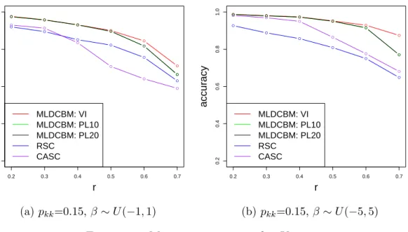
Figure 2.2: Mean accuracy vsr for K = 2, β ∼U(−1,1)

under a specific setting.

We generate θi from Beta(1,5) distribution to approximate the Power-law degree

distribution often found in real network data. Then we set theBab =ωwithin fora=b

and Bab = rωwithin where r is a number between 0 and 1. The ωwithin controls pkk,

the mean number of edges between a pair of nodes within a group while r controls the inter-community edge density pk`. We generate covariates independently from

standard normal distribution and generate the logistic regression coefficients β from uniform distribution centered at 0. We change ωwithin with β fixed to see how does

edge density affect the performance and change β with ωwithin fixed to evaluate the

impact of the level of information contained in the covariates. We tested the model with K = 2, n = 200, p = 5, and K = 5, n = 500, p = 10, and take the average accuracy of clustering over 50 repetitions under each setting. In the figures our al-gorithms are labeled as “MLDCBM”, which stands for “Multinomial Logistic Degree Corrected Blockmodel”. Further, “VI” is short for “Variational Inference” and “PL” is short for “Pseudo Likelihood”.

(37)

● ● ● ● ● ● 0.2 0.3 0.4 0.5 0.6 0.7 0.2 0.4 0.6 0.8 1.0 r accur acy ● ● ● ● ● ● ● ● ● ● ● ● ● ● ● ● ● ● ● ● ● ● ● ● MLDCBM: VI MLDCBM: PL10 MLDCBM: PL20 RSC CASC (a)pkk=0.15, β ∼U(−1,1) ● ● ● ● ● ● 0.2 0.3 0.4 0.5 0.6 0.7 0.2 0.4 0.6 0.8 1.0 r accur acy ● ● ● ● ● ● ● ● ● ● ● ● ● ● ● ● ● ● ● ● ● ● ● ● MLDCBM: VI MLDCBM: PL10 MLDCBM: PL20 RSC CASC (b) pkk=0.15,β ∼U(−5,5)

Figure 2.3: Mean accuracy vs r for K = 2

Figure 2.2 shows the result for 2 clusters and β ∼ U(−1,1) with pkk being 0.05 and

0.2 respectively. It can be seen that the proposed methods in general perform better than RSC and CASC. There is no obvious difference betweenT = 10 and T = 20 for the pseudo likelihood algorithm, which suggests the algorithm converges and the re-sults suggest that pseudo likelihood algorithm works well in most cases. It should be mentioned that CASC itself is not necessarily asymptotically consistent, which may explain its inferior performance comparing to RSC in terms of clustering accuracy. As the graph becomes denser, the accuracy of clustering should become higher in general since the networks are more informative. Figure 2.3 shows the result for 2 clusters with pkk fixed at 0.15 and β varies. The superior performance of our methods over

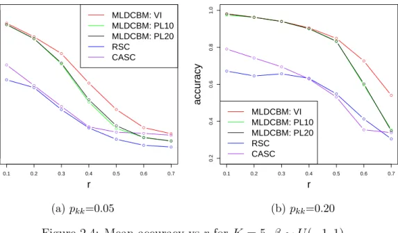
RSC becomes more significant when β increases, which is natural as the covariates are more informative with larger β. Similar results are observed for 5 clusters and are shown in Figure 2.4 and Figure 2.5.

(38)

● ● ● ● ● ● ● 0.1 0.2 0.3 0.4 0.5 0.6 0.7 0.2 0.4 0.6 0.8 1.0 r accur acy ● ● ● ● ● ● ● ● ● ● ● ● ● ● ● ● ● ● ● ● ● ● ● ● ● ● ● ● MLDCBM: VI MLDCBM: PL10 MLDCBM: PL20 RSC CASC (a)pkk=0.05 ● ● ● ● ● ● ● 0.1 0.2 0.3 0.4 0.5 0.6 0.7 0.2 0.4 0.6 0.8 1.0 r accur acy ● ● ● ● ● ● ● ● ● ● ● ● ● ● ● ● ● ● ● ● ● ● ● ● ● ● ● ● MLDCBM: VI MLDCBM: PL10 MLDCBM: PL20 RSC CASC (b) pkk=0.20

Figure 2.4: Mean accuracy vs r for K = 5, β ∼U(−1,1)

on the initialization, in the case when RSC cannot give better initial labels than pure guessing, the algorithms do not perform well and may not converge. Also, the performance of the pseudo likelihood algorithm for K = 5 is not as competitive as variational EM whenr is big. It might be suggesting that the pseudo likelihood algo-rithm is more sensitive to the initialization comparing to variational EM in the case where signal is weak.

Figure 2.6 shows the case where the relation between covariates and community labels does not follow the logistic regression structure. For 2.6(a), the dependency struc-ture between the community label and the covariates forms a mixstruc-ture model where the covariates are generated from Gaussian distributions with mean 0 or 1 depend-ing on which community the node is in. We can see that our method works better than CASC when the network is informative but the performance is not as competi-tive when the network becomes less informacompeti-tive. A possible reason is that when the network is uninformative, the initialization using RSC leads to a poor initial β esti-mate, which makes it difficult for the algorithm to utilize the covariates information

(39)

● ● ● ● ● ● ● 0.1 0.2 0.3 0.4 0.5 0.6 0.7 0.2 0.4 0.6 0.8 1.0 r accur acy ● ● ● ● ● ● ● ● ● ● ● ● ● ● ● ● ● ● ● ● ● ● ● ● ● ● ● ● MLDCBM: VI MLDCBM: PL10 MLDCBM: PL20 RSC CASC (a)pkk=0.15, β ∼U(−1,1) ● ● ● ● ● ● ● 0.1 0.2 0.3 0.4 0.5 0.6 0.7 0.2 0.4 0.6 0.8 1.0 r accur acy ● ● ● ● ● ● ● ● ● ● ● ● ● ● ● ● ● ● ● ● ● ● ● ● ● ● ● ● MLDCBM: VI MLDCBM: PL10 MLDCBM: PL20 RSC CASC (b) pkk=0.15,β ∼U(−5,5)

Figure 2.5: Mean accuracy of clustering vs r for K = 5

● ● ● ● ● ● ● 0.2 0.3 0.4 0.5 0.6 0.7 0.8 0.2 0.4 0.6 0.8 1.0 r accur acy ● ● ● ● ● ● ● ● ● ● ● ● ● ● ● ● ● ● ● ● ● ● ● ● ● ● ● ● MLDCBM: VI MLDCBM: PL10 MLDCBM: PL20 RSC CASC

(a)pkk=0.15, covariates from mixture

● ● ● ● ● ● ● 0.2 0.3 0.4 0.5 0.6 0.7 0.8 0.2 0.4 0.6 0.8 1.0 r accur acy ● ● ● ● ● ● ● ● ● ● ● ● ● ● ● ● ● ● ● ● ● ● ● ● ● ● ● ● MLDCBM: VI MLDCBM: PL10 MLDCBM: PL20 RSC CASC (b)pkk=0.15, covariates independent

(40)

● ● ● ● ● ● ● 0.2 0.3 0.4 0.5 0.6 0.7 0.8 0.2 0.4 0.6 0.8 1.0 r ● ● ● ● ● ● ● ● ● ● ● ● ● ● ● ● ● ● ● ● ● ● ● ● ● ● ● ● balanced accur acy MLDCBM: VI MLDCBM: PL10 MLDCBM: PL20 RSC CASC

Figure 2.7: Mean balanced accuracy vs r for K = 2 with unbalanced communities, pkk=0.15, β = 1

correctly. Similar to previous results, we observe that the accuracy of the pseudo likelihood algorithm drops more when r becomes larger. For 2.6(b), the covariates are generated independently from the community label, the result suggests that our methods still work well when the networks are informative although the covariates are irrelevant.

We further consider the case when the communities are unbalanced. We simulate data from the proposed model with β set to 1 and covariates from N(0.5,1). Under this setting, about 18.8% of nodes are in the minority community with a standard error of roughly 3%. Figure 2.7 shows the balanced accuracy, which is the average of sensitivity and specificity. The result shows that our methods have better perfor-mance when the network is informative and there is no obvious difference between the variational EM algorithm and the pseudo likelihood algorithm.

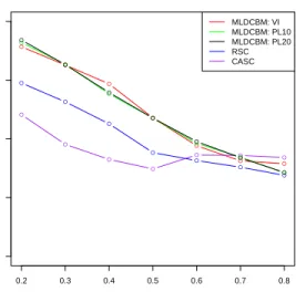
Another setting that we are interested in is when the network is not assortative, where nodes are more likely to form an edge if they are not from the same community. We

(41)

● ● ● ● ● ● ● 0.2 0.3 0.4 0.5 0.6 0.7 0.8 0.2 0.4 0.6 0.8 1.0 r accur acy ● ● ● ● ● ● ● ● ● ● ● ● ● ● ● ● ● ● ● ● ● ● ● ● ● ● ● ● MLDCBM: VI MLDCBM: PL10 MLDCBM: PL20 RSC CASC

Figure 2.8: Mean accuracy vs r for K = 2 with non-assortative networks, initialized with CASC, pk`=0.15

simulate data from the proposed model under the same setting as Figure 2.3(a) except that here we set pk` = 0.15 and pkk=rpk`. It is known that spectral clustering does

not perform well on non-assortative network while CASC still has a reasonable per-formance (Binkiewicz et al., 2014). Since our algorithms rely on the initialization, we decide to use the CASC result as the initialization under the non-assortative setting. Figure 2.8 shows the clustering accuracy. The result suggests that our method can still improve the community detection result given by CASC even when the networks are non-assortative.

Lastly, Table 2.1 shows the computing time of the proposed algorithms under the setting K = 5, n = 500, p = 10, pkk = 0.15, r = 0.4. It can be seen that pseudo

likelihood algorithm is computationally much more efficient than the variational EM and CASC.

(42)

Algorithm PL10 PL20 VI CASC Time (secs) 2.23 3.98 34.37 22.10

Table 2.1: Mean computation time of community detection algorithms under degree corrected blockmodels with covariates over 10 replications

2.6 Data example

We applied our method to a friendship network of 71 lawyers in a Northeastern US corporate law firm in New England(Lazega, 2001). The dataset also contains infor-mation on seven covariates including status, gender, office, year with the firm, age, practice, and law school. We notice there are only 4 people in the Providence office, which might not be informative as a source for dividing the network into clusters since the number of people in the office is too small comparing to 19 of the Hartford office and 48 for the Boston office. Thus we removed these 4 people and left with 67 people in the following analysis. The original network is directed with an edge from i to j if person i nominates person j as a friend. We converted it to an undirected network by letting person i and j be connected if either one of them nominates the other as a friend.

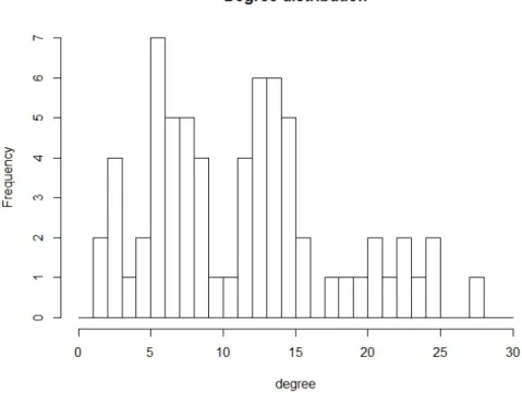
The covariates status, gender, office, practice, and law school are categorical and basically balanced between each category. The covariate year varies from 1 to 32 and has a median 7. The covariate age ranges from 26 to 67 with median 38. The degree distribution of the undirected network is shown in Figure 2.9.

We applied the variational EM algorithm and the pseudo likelihood algorithm with K = 3 and obtained same clustering result. The result is shown in Figure 2.10. Fig-ure 2.10a shows the community membership given by the algorithm. In FigFig-ure 2.10b, the colors of the nodes represent office information and the node size is proportional

(43)

Figure 2.9: Degree distribution

to years plus 10. It can be seen that community 1 contains people only from Hart-ford office, and people from Boston office are divided into 2 clusters by their years in the firm. Colors of nodes in Figure 2.10c show the status information and the node size is proportional to the age. It can be seen that nodes in community 2 are all associates and community 3 mainly consists of partners. Also, nodes in community 2 are younger comparing to community 3. We then calculated mean degree of each community. It turns out that the mean degree of community 3 is 15, which is much higher than 9.4 of community 1 and 10.3 of community 2. This is in some sense ex-pected since the senior partners in a same office may have worked with each other for many years. To summarize, the nodes are separated into 3 communities, community of people from Hartford office, community of young associates in Boston office, and community of senior partners in Boston office.

(44)

(a) Community membership

(b) Covariate: office and years (c) Covariate: status and age

(45)

2.7 Discussion

We have considered the community detection problem for networks with node covari-ates based on a principled statistical model combining the degree-corrected stochastic blockmodel and the logistic regression model. We have developed efficient estimation algorithms via the variational EM and the pseudo likelihood and illustrated their good performance in simulation studies and on a real-world data. We have also stud-ied the asymptotic properties of the pseudo likelihood algorithm and obtained weak consistency result under mild assumptions.

Regarding future work, various directions might be considered. As mentioned, the model can be extended to the case where the relation between the community labelC and node covariatesX is specified by a mixture model P(X|C). In the case where we have some prior knowledge that the covariates might be from mixtures of some distri-butions, the model may have better performance. Another perspective that naturally arises is the semi-supervised setting. If we already observe a part of the community labels of the nodes in the network, how do we estimate the unobserved community labels? The semi-supervised setting has many real-world applications especially in social networks where we may have a survey on a fraction of the targeting people on their community labels and need to inference for the others’. Going further from semi-supervised setting, we may consider the supervised setting where all the com-munity labels are known and our target is to make predictions on new nodes. This can be viewed as a network information assisted classification problem which might be of interest when the response variables in classification are dependent of each other and the dependency structure is given by a network.

From the theoretical perspective, the consistency of variational inference under the degree corrected blockmodel remains unknown, although it is natural to conjecture

(46)

so as the maximum profile likelihood has shown to be consistent without covariates. Also, we observed from simulations that the covariates do help improve the cluster-ing performance although the degree-corrected blockmodel itself without covariates provides label consistency in the asymptotic setting. It is thus interesting to study how helpful it is to incorporate covariates in non-asymptotic settings.

(47)

CHAPTER III

Missing Data Imputation with Network

Information

3.1 Introduction

Missing data problem is widely encountered in real-world data analysis. One com-monly used technique for handling missing data is imputation since most statistical procedures and algorithms rely on complete data. Thus it is essential to develop appropriate imputation procedures that produce imputations with high quality.

Many imputation methods have been proposed to handle univariate and multivariate missing data using only the information within the data set. However, in modern datasets, together with the traditional multivariate data, networks representing the relations between the entities are often also collected, where nodes in the network represent entities and edges between the nodes represent relations between the enti-ties. With real-world networks, it is widely observed that there is always some kind of cohesion effect between connected entities, i.e. the connected entities have similar covariates.

(48)

to the multivariate data set, we also observe a network between the observations that provides information on the affinity. One example is the online social network, where we observe the friendship network between the users, but only partially observe co-variates such as age, gender, income etc. for each user. The administrator of the platform may wish to impute the missing information of the users. To the best of our knowledge, this problem is not well addressed by existing imputation methods.

3.1.1 Missing data imputation methods

In the simple setting of imputing a single variable, many methods have been pro-posed and well studied. These methods can be conceptually divided into two groups, regression-based methods and hot-deck methods. Imputation through regression-based methods is straightforward. For example, one may perform a univariate regres-sion, potentially with generalized linear models or nonparametric models, and also deal with post-processing such as a necessary truncation. Once the regression model is fitted, the predicted values for the missing entries may be used as imputation. See Van Buuren (2018) (Chapter 3) for a more detailed review. The hot-deck methods, similar to nearest-neighbor methods, typically define a distance metric between two observations using the observed covariates, and the imputation for a missing value will be borrowed from a completely observed observation that is close under the met-ric. Andridge and Little (2010) provides a review on some commonly used hot-deck methods.

Imputation for multivariate missing data can be roughly divided into two categories. A joint modeling approach would model the observed and missing variables through some joint distribution, e.g. the multivariate normal or t-distribution. See Murray et al. (2018) for a comprehensive review for such kind of methods. Although joint

(49)

modeling methods are easy to understand and typically have good theoretical prop-erties, they are restrictive in many data analysis settings due to its lack of flexibility in handling complex mixed type of variables (Van Buuren, 2007).

Comparing to the joint modeling approach, the fully conditional specification is a more flexible framework for multivariate imputation (Van Buuren, 2007). Specifically, one specifies the conditional model for each variable conditioning on all other vari-ables. For multivariate imputation, an iterative imputation procedure that starts with some simple imputation and then conducts univariate imputations using the speci-fied conditional models sequentially is often used (Buuren and Groothuis-Oudshoorn, 2010). The iterative imputation procedure could be viewed as a Gibbs sampler from a Bayesian perspective: in each iteration, the sampler draws from the conditional dis-tribution on the missing entries. The specified conditional models are also flexible. In principle, one may specify any existing univariate regression model according to their need. People have studied the performances of using Predictive-Mean Matching (Bu-uren and Groothuis-Oudshoorn, 2010), Classification and Regression Tree (Burgette and Reiter, 2010), Support Vector Machines (Wang et al., 2006), and the Random Forest (Stekhoven and B¨uhlmann, 2011), ect.

Despite the flexibility of the fully conditional specification framework, there is limited result on the convergence property of the framework. Liu et al. (2013) compared the iterative imputation that uses a set of Bayesian regression modelsg as the conditional distributions to a proper MCMC algorithm under a joint modelf. They showed that under the assumption that both Markov chains have unique stationary distributions, the iterative imputation has the same stationary distribution as the joint model pro-vided that the conditional models g are compatible with f. Zhu and Raghunathan (2015) showed the convergence of the iterative imputation algorithm without the

(50)

as-sumption of requiring unique stationary distributions, but under the setting that each observation can have only one missing entry.

3.1.2 Network models

A network can be represented using an adjacency matrixA, whereAuvcould be binary

indicating whether there is an edge between nodes i and j, or weighted indicating the strength of the connection between nodes u and v. Many network models have been proposed to model a network alone, without relating to covariates, including stochastic block models (Holland et al., 1983), and exponential random graph (Robins et al., 2007) etc. SeeGoldenberg et al.(2010) for a detailed review of such models. The latent space model (Hoff, 2005; Hoff et al., 2002) provides a natural way of relating the edges in a network to covariates. In one form of the latent space model, the probability of having an edge between nodesuandvdepends on their latent positions Zu,Zv, their individual connectivity parametersbu,bv, the edge related covariatexuv,

and model parameters. Specifically, conditional on the above mentioned quantities, the probability between nodes u and v is given by

logit[P(Auv= 1)] =αxuv+bu+bv+ZuTZv.

The latent space models are flexible in the sense that they can be easily modified to cover a wide range of commonly observed network properties such as degree het-erogeneity, transitivity etc. Recently Ma and Ma (2017) developed gradient based algorithms that can fit the latent space model efficiently instead of using computa-tionally expensive MCMC algorithms.

(51)

3.1.3 Imputation with networks

In the setting where a network is observed and each node has a categorical label with some node labels being unobserved, heuristics such as label propagation (Zhur and Ghahramanirh, 2002) has been proposed to infer the unobserved labels. Starting with some initialization, label propagation iteratively assigns each node with unobserved label the label that dominates in its neighbors and iterates until convergence. This could be viewed as imputing a single categorical variable with network information. Chakrabarti et al. (2017) proposed a model that can simultaneously infer multiple missing labels on a network by encouraging each edge in the network to be explained by at least one common label. However, such methods can only be applied to cate-gorical variables, and do not take advantage of the correlation among the variables.

The main contribution of this work is that we propose an imputation method that can flexibly impute mixed type missing data while taking the network information into consideration. The idea of the method relies on combing the full conditional specification framework and the network model.

The rest of the chapter is organized as follows: Section 3.2 introduces the proposed model and method for missing data imputation with network information available; Section 3.3 provides theoretical results of the framework under a similar setting toLiu et al. (2013); Sections 3.4 and 3.5 illustrate the performance of the proposed frame-work using simulated studies and a real-world data example respectively; Section 3.6 discusses limitations and extensions of the framework.

(52)

3.2 Model and method

Our proposed imputation method builds on the full conditional specification frame-work that imputes one variable at a time, and we consider modeling the netframe-work using a latent space model conditional on the covariates.

Suppose we observe an incomplete data matrixXwithnobservations andpvariables. Together with X, we observe a network characterized by its n×n binary adjacency matrix A that represents connectivity between the observations.

Let Xj denotes the j-th variable and X−j denotes the other variables. Let Xj be

the variable we are imputing in the current iteration, Mj ⊂ {1,2, ..., n} denotes the

set of indices ifor which Xij is missing, andOj ={1,2, ..., n}\Mj be the index set for

the observed. Our target is to impute all missing entries {Xij, i∈Mj, j = 1,2, ..., p}

using information from A and {Xij, i∈Oj, j = 1,2, ..., p}.

We assume the network is generated from a latent space model conditional on X:

auv:=logit(P(Auv = 1|X)) = p

X

j=1

αjd(Xuj, Xvj) +bu+bv+ZuTZv

with parametersα= (α1, ..., αp)T,b= (b1, ..., bn)T and latent positionsZ = (Z1, Z2, ...Zn)T.

The overall algorithm contains the following steps:

(i) Initialize the imputation using some imputation methods. Fit the latent space model using the imputed X to initialize the model parameters and the latent positions.

(53)

X−j fixed.

(iii) Update the model parameters and latent positions. (iv) Iterate between steps (ii) and (iii) until convergence.

For the remaining of the chapter, we set d(Xuj, Xvj) = (Xuj −Xvj)2 for continuous

variables and d(Xuj, Xvj) = 1(Xuj6=Xvj) for discrete variables. Other choices of the

distance measure are also possible and will be discussed.

Without loss of generality, we consider the problem of imputing X1 with other

vari-ables, the latent space model parameters, and the latent positions fixed. The general framework of imputation proceeds as follows. Suppose we are given the conditional distribution of the missing entries P({Xu1, u ∈ M1}|X−1,{Xv1, v ∈ O1}), possibly

specified by a regression model, we may consider the following criterion:

maxP(A,{Xu1,u∈M1}|X−1,{Xv1, v ∈O1})

= maxP(A|X1, X−1)P({Xu1,u∈M1}|X−1,{Xv1, v ∈O1})

(3.1)

One interpretation of this criterion is that we have a prior on the missing entries {Xu1,u∈M1}given byP({Xu1,u∈M1}|X−1,{Xv1, v ∈O1}), with likelihoodP(A|X1, X−1),

(54)

3.2.1 Imputation of continuous variables

Suppose X1 is a continuous variable, with all the other variables X−1 fixed, the

conditional log likelihood of the network is

logP(A|X1, X−1) = X u,v α1(xu1−xv1)2Auv −X u,v log ( 1 + exp[α1(xu1−xv1)2+ p X j=2 αjd(xuj, xvj) +bu+bv+ZuTZv] ) +X u,v p X j=2 αjd(xuj, xvj) +bu+bv+ZuTZv Auv.

Note that the terms in the last line do not depend on {xu1, u∈M1}.

Suppose the specified conditional distribution P({xu1, u ∈ M1}|X−1,{xv1, v ∈ O1})

has the form such that foru∈M1,xu1|x{u,−1} ∼N(ˆxu1, σ2), then the general criterion

(3.1) has the following form

max xu1,u∈M1 ( X u,v α1(xu1−xv1)2Auv −X u,v log " 1 + exp[α1(xu1−xv1)2+ p X j=2 αjd(xuj, xvj) +bu+bv+zuTzv] # − 1 2σ2 X u∈M1 (xu1−xˆu1)2 ) . (3.2)

When σ is unknown, we may replace the term _2σ12 with an estimate or a specified

(55)

specified conditional distribution, and obtain the following criterion max xu1,u∈M1    X (u,v) α1(xu1−xv1)2Auv −X u,v log " 1 + exp[α1(xu1−xv1)2+ p X j=2 αjd(xuj, xvj) +bu +bv+ZuTZv] # −λX u∈M (xu1−xˆu1)2 )

The solution to this optimization problem is then an imputation of {xu1, u ∈ M1}.

We may use gradient based methods to compute the solution with gradient in the following form. ∂ ∂xu1 = X v 2α1(xu1−xv1)Auv− X v 2α1(xu1−xv1)σ(auv)−2λ(xu1−xˆu1) = 2α1hAu−σ(au), xu11n−x·1i −2λ(xu1−xˆu1),

where Au is the u-th row of A and a= (auv)u,v≤n with au being theu-th row, σ(·) is