Modeling Survival Times using Frailty Models
Liberato Camilleri, Roxanne Caruana, Alex Manche’ Department of Statistics and Operations Research
University of Malta Msida (MSD 06) Malta E-mail: [email protected]
KEYWORDS
Heterogeneity, Shared and Unshared Frailty models, Kaplan Meier, Nelson Aalen, Cox Regression models.
ABSTRACT
Traditional survival models, including Kaplan Meier, Nelson Aalen and Cox regression assume a homogeneous population; however, these are inappropriate in the presence of heterogeneity. The introduction of frailty models four decades ago addressed this limitation. Fundamentally, frailty models apply the same principles of survival theory, however, they incorporate a multiplicative term in the distribution to address the impact of frailty and cater for any underlying unobserved heterogeneity. These frailty models will be used to relate survival durations for censored data to a number of pre-operative, operative and post-operative patient related variables to identify risks factors. The study is mainly focused on fitting shared and unshared frailty models to account for unobserved frailty within the data and simultaneously identify the risk factors that best predict the hazard of death.
1. Introduction
Survival analysis is a useful statistical method for answering questions that deal with the duration of events. Survival models have been used in several research fields to analyze data involving time to a certain event such as death, relapse and onset of a disease. Essentially the duration of a study is treated as the dependent variable and therefore proper definition of the investigation period plays a vital role in determining the number of deaths.
Although there are several types of non-parametric (Kaplan Meier and Nelson Aalen), semi parametric (Cox regression) and parametric techniques to analyze the survival times, these methods do not cater for unobserved heterogeneity. The introduction of frailty models overcomes this limitation. Fundamentally the same principles from survival theory apply, however a multiplicative term is incorporated in the distribution being considered in order to model the impact of frailty.
These models provide a novel approach to survival problems and they encompass two main types of models, namely the unshared and the shared frailty models. In the unshared case a dataset is analyzed assuming that each individual has an associated distinct random effect. The shared case assumes that persons sharing a common factor, such as children born to the same mother or patients with a common health condition,
may be analyzed group-wise. Entities within each group are assigned the same frailty effect, but varying heterogeneity levels are expected to subsist among the clusters.
The word frailty was first coined by Vaupel et al., (1979) where it was presented in their research on mortality and later extended by Hougaard (1984). They illustrated that although individuals appear physically alike, they have different threats independently associated to them. In 1984, Hougaard further observed that the difference between the Gamma and Inverse Gaussian distributions is derived from frailty instability among those still alive. In the former case frailty remained steady but in the latter case frailty dropped as individuals grew older. It was further noticed that the random effect had an impact on the hazard equation, which led to the concept that frail persons are bound to decline faster. This unobserved random effect is discussed by several authors in various papers.
Frailty techniques are generally employed to estimate the variance of unobserved risks among individuals. In the univariate scenario, a frailty is assumed to have a unit mean and variance and operates multiplicatively on the baseline hazard. Failure times of particular occurrences are the central purpose for such analysis, as the interest lies in understanding the proneness to some specific occurrence, such as illness. For instance one might be concerned with the recurrence times of smoking after withdrawal, or the time it takes until heart failure sets in. Most often in clinical applications, frailty may be regarded as a means of describing the biological age rather than the chronological age, due to various factors. The utility of shared frailty models was first highlighted by Clayton and Cuzick in the 70’s where the authors emphasized the added benefit of including frailty when heterogeneity impact is common among individuals within a group. Each set has a distinct random effect, which in turn causes frailties to be interrelated. Furthermore, the distinction between a frailty model in the shared and the unshared case lies in the hazard function. Hougaard, and Whitmore & Lee enhanced developments on shared frailty models by addressing frailty by assuming a Weibull baseline hazard function and an Inverse-Gaussian frailty distribution. Flinn and Heckman in 1982 also made use of the lognormal distribution to address frailty.
Shared proportional hazard techniques were introduced primarily through the works of Therneau et al. (2000) and Ripatti and Palmgren (2000). These researchers implemented the penalized partial likelihood (PPL) method to elicit results on frailty models using either a Gamma or an Inverse Gaussian distribution. Subsequently in 2003, Klein and Moeschberger
presented an alternative approach to the PPL method by proposing the application of the expectation-maximization (EM) algorithm. The idea was to determine the variances of the maximum likelihood estimates from the information matrix. Moreover Therneau et al. (2003) proved a very important result, namely that the EM and PPL methods produce equivalent results for the gamma distribution. In fact this was confirmed in their studies which were implemented both in SAS and R.
In 2008, Jenkins developed an algorithm for STATA that allowed the inclusion of a univariate frailty term for discrete event times. He showed that despite the fact that the data comprises discrete event times it is possible to obtain reliable results similar to the continuous parametric techniques. A weakness of this method is that the heterogeneity term is only assumed to have a gamma or a normal distribution. Hence it is only possible to compare between discrete and continuous gamma frailty models. Some of the outstanding works on frailty used in this paper include Wienke (2011), Duchateau and Janssen (2008), Hanagal (2011), and Kleinbaum and Klein (2005).
2. Theory of unshared frailty models
The seminal work of Clayton and Cuzick in the late 70’s highlighted the utility of shared frailty models and stressed the added benefit of adding frailty when examining associations between models. As highlighted in the introduction, there are
two types of frailty models to analyze survival data in the presence of unobserved heterogeneity. In unshared frailty models, the frailty is introduced at the observation level as an unobservable multiplicative effect, α on the baseline hazard function h t0( ) such that:
( )
0( )
h tα =αh t (1) In this context, α is a non-negative random mixture variable where E( )α =1 and var( )
α
=σ
2. When σ2is small, the values of α are located close to 1; however the values ofαare more dispersed when σ2is large, inducing larger heterogeneity in the individual hazards αh t0( ).Let S t( α) denote the survival function of a life conditional on the frailty α and let 0 0
0 ( ) ( ) t h s ds=M t
∫
then( )
0 ( ) 0 0( ) 0( ) t t h s ds h s ds M t S tα =e−∫ α =e−α∫ =e−α (2)If observed covariates
X
are available then the hazard is proportional to the baseline hazard, where the constant of proportionality is the exponential term exp( ' ).β X So model (1) becomes:(
,)
0( )
exp( ' ) h t Xα =αh t β X (3) whereX=( ,x1 …,xp)and 1 (β , ,βp) = β … is the vector of regression parameters.The two distributions that are normally considered for the probability density function f( ),α of αare the gamma and inverse Gaussian distributions.
Given the simple Laplace transform of the Gamma distribution ( , ),k λ
Γ it is easy to derive the closed-form expressions of the survival and hazard functions. The exponential distribution is a special case of the Gamma distribution when the shape parameter k=1. If α has a Gamma distribution and α>0,
0,
λ> k>0 its probability density function is given by:
( )
( )
1 k k f e k λα λ α = α − − Γ (4) By setting k= =λ 1/σ2 ensures that the model is identifiable and ensures that E( )α =1 and var( )α
=σ
2. Moreover, the unconditional survival and hazard functions are given by:( )
2 1 2 0 1 ( ) 1 S t M t σ σ = + (5)( )
0 2 0 ( ) ( ) 1 h t h t M t σ = + (6)Moreover, if observed covariates
x
i are available for life ithen the mean frailty and frailty variance for a life dying beyond time t are given by:
( )
2 0 1 ( , ) 1 exp( ' ) E T t M t α σ > = + X β X (7) 2 2 2 2 0 (1 ) var( , ) 1 ( ) exp( ' ) T t M t σ σ α σ + > = + X β X (8)The Inverse Gaussian distribution is also considered as a frailty distribution because similar to the Gamma distribution, simple closed-form expressions exist for the unconditional survival and hazard functions. If α has an Inverse Gaussian distribution and α >0, λ>0, µ>0 its probability density function is given by:
( )
3 2 2 ( ) exp 2 2 f α λ λ α µ µ α πα − = − (9)By setting µ=1 and λ=1/σ2 guarantees that the model is identifiable and ensures that E( )α =1 and var( )
α
=σ
2. The unconditional density function, the unconditional survival and hazard functions are given by:( )
2 0 2 1 1 2 ( ) exp M t S t σ σ − + = (10)( )
0 2 0 ( ) ( ) 1 2 h t h t M t σ = + (11)If observed covariates
x
i are available for life i then the mean frailty and frailty variance for a life dying beyond timet are given by:
( )
2 0 1 ( , ) 1 exp( ' ) E T t M t α σ > = + X β X (12) 2 2 2 0 var( , ) 1 ( ) exp( ' ) T t M t σ α σ > = + X β X (13)Possible choices for baseline hazard include the exponential, Weibull, Gompertz, log-normal and log-logistics distributions.
3. Theory of shared frailty models
A generalization of the unshared frailty model is the shared frailty model, where the frailty is assumed to be group-specific. Basically shared frailty arises when the heterogeneity impact is common among individuals within a group, yet each set has a distinct random effect, which in turn causes frailties to be interrelated.
Suppose there exist n groups and that group i comprises
n
iobservations associated with the unobserved frailty αifor 1≤ ≤i n. Their hazard functions are given by:
( )
i i 0( )
h tα =αh t (14) Let S t( αi) denote the survival function of a life conditional
on the frailty αiand let 0 0
0 ( ) ( ) ij t ij h s ds=M t
∫
then(
1)
0 1 ,..., exp ( ) i i n i in i i ij j S t tα
α
M t = = − ∑
(15)If observed covariates
X
i for 1≤ ≤i n are available then the hazard is proportional to the baseline hazard, where the constant of proportionality is the exponential term exp( ' ).β XAssuming that the survival times in group i are independent, then model (16) becomes:
(
i, i)
i 0( ) exp( ' i) h t X α =αh t β X (16) where ( 1, , ) i i = i in X x … x and 1 (β , ,βp) = β … is the vector of regression parameters. The conditional survival function on frailty αiwhich is shared by all individuals in group i is given by:(
)
' 1 0 1 ,..., , exp ( ) i ij i n i in i i i ij j S t tα
α
M t e = = − ∑
βx X (17)The Gamma and Inverse Gaussian frailty models are often used mainly for their nice properties, particularly their simple Laplace transform. Popular choices for the baseline hazard include the Weibull and Gompertz distributions.
4. Application
The dataset used for the frailty model application comprised 365 Maltese patients who underwent aortic valve replacement from 1995 to 2014 at the cardiothoracic centre in a Maltese hospital. Although the ages of the patients ranged from 15 to 87, the vast majority were over 60. In fact it is well known that the risk of requiring heart surgery increases with age. All the patients were followed up after the operation. For those who died, the time of death was recorded in order to compute their survival duration. The majority of the patients were still alive by the end of the investigation period, and their survival times were set equal to the duration between the operation and the end of the investigation period. This type of censoring is non-informative, where observations are right censored.
The data for each patient was recorded by the surgeon conducting the operation. The predictors involved included pre- and post-operative factors, demographic and other patient related explanatory variables. Essentially, the dependent variable, Time is the survival duration after surgery recorded on a continuous scale. The variables Status is categorical indicating whether the patient died or survived by the end of the investigation period. This variable will be used to identify the censoring status of each patient.
The Logistic Euroscore estimates the predicted operative mortality for patients undergoing cardiac surgery. This risk measure of death has a metric scale. Mechanical+Graft is a categorical variable indicating the presence or absence of a mechanical valve during surgery with concomitant coronary artery bypass grafting. Xeno+Graft is a categorical variable indicating the presence or absence of a biological valve with artery grafting. The variable Bleeding records the blood volume, in millilitre, lost post-operatively until removal of chest drains. The variable Transfusion records the number of blood units transfused, where 1 unit corresponds to 250ml of blood.
IABP
is a categorical variable indicating whether an intra-aortic balloon pump was required to assist the heart to pump. Dialysis is a categorical variable indicating whether the patient was on dialysis due to kidney failure after the operation and the patient’s Age is measured in years. CTS records the duration of patients in the central treatment suite after heart surgery. It is a categorical variable (1-4, 5-10, 11-16, 17 days or more) and will be used as the grouping variables in the shared frailty models.5. Results of the unshared frailty models
All the fitted models in this section are implemented as proportion hazard models and assume a Gompertz baseline hazard function given by:
( )
0 = j t j h t λ eγ(18) where λj=exp
(
β0+β1 1x + +... βpxp)
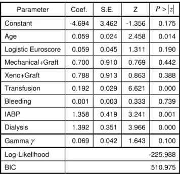
and γ is an ancillaryparameter. Table 1 displays the parameter estimates, standard errors and p-values of the non-frailty model.
Table 1: Estimates of non-frailty model
Parameter Coef. S.E. Z P> z
Constant -4.694 3.462 -1.356 0.175 Age 0.059 0.024 2.458 0.014 Logistic Euroscore 0.059 0.045 1.311 0.190 Mechanical+Graft 0.700 0.910 0.769 0.442 Xeno+Graft 0.788 0.913 0.863 0.388 Transfusion 0.192 0.029 6.621 0.000 Bleeding 0.001 0.003 0.333 0.739 IABP 1.358 0.419 3.241 0.001 Dialysis 1.392 0.351 3.966 0.000 Gammaγ 0.069 0.042 1.643 0.100 Log-Likelihood -225.988 BIC 510.975
The non-frailty model identifies four significant predictors of survival duration. The parameter estimate of Age (0.059) indicates that for every 1-year increase in age the hazard of death increases by 6.1%; the parameter estimate of Transfusion (0.192) indicates for every 1-unit increase in transfused blood the hazard of death increases by 21.1%. The parameter estimate of IABP (1.358) indicates that for patients requiring anintra-aortic balloon pump after heart surgery the hazard of death is 3.89 times in patients who do not require this device. The parameter estimate of Dialysis (1.392) indicates that for patients on dialysis due to kidney failure the hazard of death is 4.02 times in patients who do not have this condition. The parameter estimates of Logistic Euroscore, Mechanical+Graft, Xeno+Graft and Bleeding are not significant because their p-values exceed the 0.05 level of significance. The log-likelihood of the non-frailty model is -225.99 and the estimate of the ancillary parameter (0.069) is not significantly different from 0.
Table 2: Estimates of unshared Gamma frailty model
Parameter Coef. S.E. Z P> z
Constant -2.839 5.142 0.552 0.581 Age 0.096 0.043 2.233 0.025 Logistic Euroscore 0.048 0.077 0.623 0.533 Mechanical+Graft 1.574 1.427 1.103 0.270 Xeno+Graft 1.873 1.872 1.001 0.317 Transfusion 0.200 0.091 2.198 0.028 Bleeding 0.011 0.008 1.375 0.169 IABP 3.895 1.066 3.654 0.000 Dialysis 3.239 1.076 3.010 0.003 Gammaγ 0.317 0.089 3.562 0.000 Log(var )α 1.957 0.355 5.513 0.000 Log-Likelihood -218.505 BIC 501.910
Table 3: Estimates of unshared Inv. Gaussian frailty model
Parameter Coef. S.E. Z P> z
Constant -2.918 5.928 -0.492 0.623 Age 0.113 0.045 2.511 0.012 Logistic Euroscore 0.093 0.077 1.208 0.227 Mechanical+Graft 0.862 1.567 0.550 0.582 Xeno+Graft 0.995 1.568 0.635 0.525 Transfusion 0.297 0.058 5.121 0.000 Bleeding 0.003 0.006 0.500 0.617 IABP 2.650 0.743 -3.567 0.000 Dialysis 2.722 0.651 -4.181 0.000 Gammaγ 0.331 0.067 4.940 0.000 Log(var )α 4.484 0.976 4.594 0.000 Log-Likelihood -216.260 BIC 497.419
To apply the theory described in section 2, unshared Gamma and Inverse-Gaussian frailty models were fitted using Stata streg directives. Table 2 and Table 3 show the parameter estimates, standard errors and p-values of these two unshared frailty models. For both models, the parameter estimates of Age, IABP, Transfusion and Dialysis are significantly positive complementing the results of the non-frailty model. Moreover, the estimates of the frailty variance of the Gamma (5.24) and Inverse Gaussian (88.59) model are both significant, which implies that the data exhibits substantial frailty. In fact, the BIC of the Inverse Gaussian (497.42) and Gamma (501.91) frailty models are considerably lower than the BIC of the non-frailty model (510.97).
6. Results of the shared frailty models
Table 4: Estimates of shared Gamma frailty model
Parameter Coef. S.E. Z P> z
Constant -4.395 3.558 -1.235 0.217 Age 0.053 0.024 2.254 0.024 Logistic Euroscore 0.043 0.045 0.945 0.344 Mechanical+Graft 0.646 0.927 0.698 0.485 Xeno+Graft 0.803 0.935 0.859 0.390 Transfusion 0.203 0.029 6.855 0.000 Bleeding 0.002 0.033 0.074 0.941 IABP 1.120 0.426 2.626 0.009 Dialysis 1.387 0.351 3.956 0.000 Gammaγ 0.081 0.040 2.025 0.044 Log(var )α 1.601 0.643 2.488 0.013 Log-Likelihood -220.813 BIC 506.525
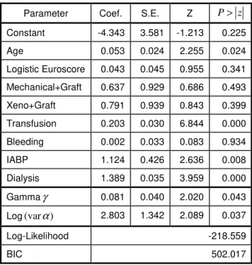
Table 5: Estimates of shared Inv. Gaussian frailty model
Parameter Coef. S.E. Z P> z
Constant -4.343 3.581 -1.213 0.225 Age 0.053 0.024 2.255 0.024 Logistic Euroscore 0.043 0.045 0.955 0.341 Mechanical+Graft 0.637 0.929 0.686 0.493 Xeno+Graft 0.791 0.939 0.843 0.399 Transfusion 0.203 0.030 6.844 0.000 Bleeding 0.002 0.033 0.083 0.934 IABP 1.124 0.426 2.636 0.008 Dialysis 1.389 0.035 3.959 0.000 Gammaγ 0.081 0.040 2.020 0.043 Log(var )α 2.803 1.342 2.089 0.037 Log-Likelihood -218.559 BIC 502.017
To apply the theory described in section 3, shared Gamma and Inverse-Gaussian frailty models were fitted using Stata streg directives. The models are implemented as proportion hazard models and assume a Gompertz baseline hazard function. Table 4 and Table 5 show the parameter estimates, standard errors and p-values of these two shared frailty models. Both models, confirm that IABP, Age, Transfusion and Dialysis are significant predictors of the hazard of death. Moreover, the estimates of the frailty variance are both significant, which indicates the presence of substantial frailty. The unshared Inverse Gaussian frailty model yields the lowest BIC value (497.42) implying that it provides the best fit. On the other, the non-frailty model yields the highest BIC value (510.98) implying that it provides the poorest fit.
6. Conclusion
This paper presents two shared and two unshared frailty models assuming a Gamma or an Inverse Gaussian frailty distribution and a Gompertz baseline hazard function. This paper shows that in the presence of heterogeneous data these models provide a significantly better fit than non-frailty ones. For this data, the Inverse Gaussian assumption for the frailty distribution provided a better fit than the Gamma distribution. An alternative approach to these parametric models is to fit semi-parametric frailty models, which do not require any assumptions on the baseline hazard function. These models can be implemented using the coxph directive in the R statistical software, where parameters are estimated using the EM (expectation maximization) algorithm, which iterates between two steps. The first step estimates the unobserved frailties and model parameters based on observed data. These estimates are used in the maximization step to obtain updated parameter estimates given the estimated frailties. The iterative procedure is continued until it converges. The likelihood includes both the observed data and unobserved
frailties, which are assumed to be random. These models can also be implemented using the frailtypack in the R package, which uses the PPL (penalized partial likelihood) approach. However, this estimation method can yield different results when compared to the coxph approach. In frailty models these techniques work best when the random effects are significant. STATA has the facility to fit semi-parametric Gamma frailty models but not Inverse Gaussian models.
References
Clayton, D. G. & Cuzick J. (1985), Multivariate generalizations of the proportional hazard model. Journal of the Royal Statistical Society A, 148(2):82–117.
Dempster, A. P., Laird, N. M. & Rubin, D. (1977), Maximum Likelihood from Incomplete Data via the EM algorithm,
Journal of the Royal Statistical Society, B, 39, 1-38.
Duchateau, L. & Janssen, P. (2008), The frailty model. New York Springer.
Flinn, C. & Heckman, J. (1982), New methods for analyzing structural models of labour force dynamics. Journal of Econometrics 18: 115-168.
Hanagal, D. D. (2011), Modeling survival data using frailty models. Chapman & Hall/CRC
Horowitz J. L. (1999), Semiparametric estimation of a proportional hazard model with unobserved hetrogeneity. Econometrica, 67(5):1001–1028.
Hougaard. P. (1984), Life table methods for heterogeneous populations: Distributions describing the heterogeneity. Biometrika, 71(1): 75–83.
Ripatti, S. & Palmgren, J. (2000), Estimation of multivariate frailty models using penalized partial likelihood. Biometrics 56: 1016-1022.
Therneau, T. M., Grambsch, P. M. &Pankratz, V. S. (2003), Penalized survival models and frailty. Computational and Graphical Statistics Journal, 12(1): 156-175.
Vaupel, J.W., Manton, K.G. & Stallard, E. (1979), The impact in individual frailty on the dynamics of mortality. Demography, 16(3), 439-454.
Wienke, A. (2010), Frailty models in survival analysis. Chapman and Hall/CRC
AUTHOR BIOGRAPHY
LIBERATO CAMILLERI studied Mathematics and Statistics at the University of Malta. He received his PhD degree in Applied Statistics from Lancaster University. His research specialization areas are related to statistical models, which include Generalized Linear models, Latent Class models, Multilevel models and Mixture models. He is an associate professor and Head of the Statistics department at the University of Malta.