Forecasting aggregate and disaggregates with common features.

(1)

Working Paper 11-08

Statistics and Econometrics Series (05) April 2011

First version: December 2011 Final version: April 2012

Departamento de Estadística Universidad Carlos III de Madrid

Calle Madrid, 126 28903 Getafe (Spain) Fax (34) 91 624-98-49

Forecasting aggregates and disaggregates with common

features

Antoni Espasa 1 and Iván Mayo 2 3

Abstract

This paper focuses on providing consistent forecasts for an aggregate economic indicator, such as a consumer price index, and all its components, and on showing that the indirect forecast of the aggregate is at least as accurate as the direct forecast. The procedure developed is a disaggregated approach based on single-equation models for the components, which take into account the stable features as common trend and common serial correlation that some components have in common. Our procedure starts by classifying a large number of components based on restrictions from common features. The result of this classification is a disaggregation map, which may also be useful in applying dynamic factors, defining intermediate aggregates or formulating models with unobserved components. We apply the procedure to forecast inflation in the Euro Area, the UK and the US. Our forecasts are significantly more accurate than a direct forecast of the aggregate and other indirect forecasts.

Key Words: Common trends; Common serial correlation; Inflation; Euro area; UK; US; Cointegration; Single-equation econometric models; Disaggregation maps

1

Antoni Espasa, Universidad Carlos III de Madrid, Statistics Department, and Instituto Flores de Lemus, C/Madrid, 126, 28903 Getafe (Madrid), Spain, phone: (34) 916249803, email: [email protected].

2

Iván Mayo, Universidad Carlos III de Madrid, Instituto Flores de Lemus, C/Madrid, 126, 28903 Getafe (Madrid), Spain, email:[email protected].

Additional results of this paper could be obtained from the first author’s website:

http://halweb.uc3m.es/esp/Personal/personas/espasa/esp/publications/ExtendedResults.html 3

This paper was originally distributed as “Forecasting A Macroeconomic Aggregate Which Includes Components With Common Trends”. We appreciate the comments and suggestions by Katerina Juselius. We are grateful for the comments of the participants at the Econometric Seminars of the Nuffield College and the European University Institute. We are also grateful to an anonymous referee for his helpful comments. Antoni Espasa acknowledges financial support from Ministerio de Educación y Ciencia, proyect ECO 2009-08100. Any opinions are solely those of the authors.

(2)

1. Introduction.

The demand for macroeconomic forecasts has increased considerably in the last twenty years and with it the requests for quicker and more detailed releases of official data. In this context, one important phenomenon is the steadily growing flow of information available to forecasters; in particular, data are increasingly becoming available at a higher degree of disaggregation—at the regional, temporal and sector levels. Therefore, the traditional debate about forecasting an aggregate variable directly or indirectly by aggregating the forecasts of its components has recently received considerable attention. Usually, this discussion concentrates only on the forecasting accuracy of the aggregate. By contrast, the starting point of this paper is that all data— aggregate and components—are relevant, both for a full understanding of the aggregate and for the formulation of useful economic policies. The focus of this paper is on inflation, but the question of the usefulness of disaggregated information for econometric modelling and forecasting is relevant for many other macroeconomic variables to which the proposals in this paper could therefore be applied.

Behind an aggregate lies a great amount of data that should not be ignored when generating the forecasting results that economic agents need for designing economic policy measures, making investment decisions and related activities. For instance, in analysing all the price components of a Consumer Price Index (CPI), a frequent observation is that several prices share features such as common trends or common serial correlation, whereas others do not, perhaps because they are affected by technological changes in a particular way or because they are affected differently by changes in preferences. Similar remarks apply when considering the specific sectorial industrial production indexes of a national industrial production index, or the individual components of aggregates such as exports and imports. In examples such as these, a valid hypothesis is that a certain subset of components of the aggregate share a common feature but others do not. Consequently, it seems convenient to use disaggregated information and exploit the restrictions existing between the components in econometric modelling in order to provide decision makers with forecasts that refer to the aggregate and its components. For example, a forecast of 2.2% for headline inflation next year with a large percentage of price components forecast to grow at around the same rate is quite different from the same forecast in which the rate of growth of energy prices is forecast at 15% and many other prices are forecast to grow at very small percentage. We advocate consideration of all, say n components of an aggregate, which we call basic components. We aim to provide joint consistent forecasts for the aggregate and its basic components as well as for useful intermediate aggregates. A validation of our proposal would involve showing that the indirect forecast of the aggregate is at least as accurate as the direct one. If an indirect forecast based on disaggregation is more accurate than a direct forecast of the aggregate, then clearly disaggregation is useful.

The literature in this area of research considers mainly three time-series forecasting procedures: (F1) the direct approach, which works with a scalar model for the time series of the aggregate; (F2) the disaggregated procedure based on univariate models for each of the basic components; and (F3) the multivariate disaggregated approach, which works with a vector model for the time series of all the basic components. A fourth alternative (F4), developed in this paper, is a disaggregated approach based on

(3)

single-equation models for the basic components that include restrictions between them. In the applications in section 5 we denote this alternative as FP4.

Theory shows that when the data generation process (DGP) is known, the forecasting accuracy of F3 is at least as good as that of the other procedures. Nevertheless, if the number of components is large, as is usually the case when working with basic components—numbering 160 in the US CPI in this study, for example—then F3 is not feasible; in any case, it would be subject to a great deal of estimation uncertainty, on which we comment below. On the other hand, F2 can be better or worse than F1 depending on the properties of the data. As will become clear, the existence of restrictions between the components is one of the main reasons why the disaggregated approach could be useful. In this paper, we develop an intermediate—in relation to F1, F2 and F3—approach, called F4, which is based on single-equation models that take into account important restrictions between the components arising from the fact that some share common features. We keep this approach simple by using bivariate methods to identify a unique common feature in a subset of components and by using single-equation models to forecast each basic component. Furthermore, the basic components that do not share common features are aggregated into an intermediate aggregate, which is forecasted directly. Our procedure differs from that used in the dynamic factor literature because we consider the possibility of common features in analysing the behaviour of each variable in relation to the others—the basic components of an aggregate—and we only estimate common features between the basic components that truly share them—the estimation restriction. Then, each factor is used only in modelling and forecasting the basic components that have the corresponding common features— the forecasting restriction. At the same time, the procedure requires that the presence of common features be stable. In the dynamic factor literature applied to a large number of series, as it is our case, all elements are considered to incorporate a common factor without the above estimation restriction, which leaves the estimation process to determine which components enter with zero weight. If application of the estimation restriction is appropriate, the common factors (features) in our procedure could be estimated more precisely in small samples and may also have a more direct economic interpretation.

Recently, Hendry & Hubrich (2006, 2010), hereafter HH, proposed a procedure for forecasting an aggregate by using a model for that aggregate that includes as regressors its own lags as well as lags of the components. They use autometrics (see Doornik, 2009), and follow the general-to-specific approach to build the model. Our procedure differs from the HH procedure in two main respects. The first arises because our procedure incorporates specific identified and tested restrictions between the basic components in forecasting the aggregate. Because their model does not include all the components in the equation for the aggregate, HH implicitly incorporate unknown restrictions between the components. However, as shown by Clark (2000), specific restrictions, such as cointegration restrictions should also be taken into account. The second difference is that our procedure naturally provides forecasts for the basic components, which are considered of interest because they could be necessary for decision makers. HH only provide results for the aggregate because, the forecasts at different horizons are made using a horizon-specific estimated models, where the dependent variable is the multi-period ahead value being forecasted, and so, they only need observed values of the independent variables.

The remainder of the paper is structured as follows. In Section 2, in relation to forecasting an aggregate, we comment on theoretical efficiency, estimation uncertainty

(4)

and the relevant restrictions. In Section 3, we describe the data, the intermediate aggregation schemes with basic components and the tests for positive and seasonal unit roots. In section 4 we present our forecasting approach and the classification of the basic components in a disaggregation map which take account of some common features between them. In Section 5, we apply our procedure to forecast inflation in the US, the Euro Area (EA) and the UK, and we compare these results with those obtained from a direct forecast, an indirect forecast based on univariate models and an indirect forecast based on models with a stationary dynamic factor. In Section 6, we draw conclusions and propose extensions for future work. The applications in this paper include a large amount of results which cannot be reported here, but the interested reader will find more details about them on the first author’s website4

.

2. Theoretical efficiency, estimation uncertainty and

relevant restrictions

Theoretical results for stationary variables—for details, see Rose (1977), Tiao & Guttman (1980), Wei & Abraham (1981), Kohn (1982) and Lütkepohl (1984) among others—have shown that, in general, procedure F3 will provide more accurate forecasts of the aggregate. It is only if the data satisfy special conditions—conditions for efficiency of the direct forecast (CEDFs)—that the direct approach is efficient; see Kohn (1982). In the case of one aggregate and n basic components, these conditions require that when applying the vector of aggregating weights to the polynomial matrix of the vector moving average (VMA) representation of the components, one obtains a vector in which all of its n elements are simply the dynamic polynomial of the MA representation of the aggregate. Similarly, the condition can also be formulated for VAR processes.

A CEDF is a very specific condition and when it does not apply, the use of the direct forecasting approach implies that invalid restrictions are imposed on the DGP—all the available data, the basic components. To avoid imposing invalid restrictions in this sense, one can work from the basic components. This is because if we break down the aggregate into a smaller number of components, which we term intermediate aggregates, these intermediate aggregates will be aggregates of basic components; then, when modelling these intermediate aggregates, one could find that invalid restrictions are being imposed on the basic components included in them. If this is the case, we can use a wider disaggregation to improve the modelling and forecasting of these intermediate aggregates and thereby forecast the overall aggregate more accurately. There is another, perhaps more important, reason for considering the basic components. Assume that a subset of basic components share a common feature. Our procedure reduces the variance of the forecasting errors of the aggregate by taking these

4

Detailed results for all these tests can be obtained from the first author’s website: http://halweb.uc3m.es/esp/Personal/personas/espasa/esp/publications/ExtendedResults.html

(5)

restrictions into account However, intermediate aggregates based on official or ad hoc breakdowns include, in general, a subset of basic components which are cointegrated plus other components which are not. Therefore when testing a pair of intermediate aggregates for cointegration, it is often found that they are not cointegrated. For instance, Espasa and Albacete (2007) show that in breakdowns of the CPI’s of different Euro Area countries into two components, Core CPI and the rest, these components are not cointegrated. In these cases, the cointegration present in the basic components cannot be exploited working with intermediate aggregates.

Lütkepohl (1987) shows that CEDFs hold, for instance, when the components are uncorrelated and have identical stochastic structures. This can be taken as an indication that when components have different distributions—for instance when some have conditional heteroskedasticity or have a conditional mean with a nonlinear structure—or when there are cross-restrictions between them, disaggregation could be important. In this paper, we limit ourselves to considering the case in which there are restrictions between the components. This does not mean that distributional differences are unimportant; it merely allows us to study the problem in a way that is easier to solve in a general framework.

Recent consideration has been given to the case in which the components are nonstationary and cointegrated. Our approach is inspired by the results of Clark (2000), who shows that, when the model is known, the indirect forecast from a vector equilibrium correction model (VEqCM) for the components is more accurate than the direct forecast. Again, it is only under very specific conditions that the two forecasts are equivalent. These conditions include ones similar to those specified by Kohn (1982) for the transitory dynamics of the VEqCM as well as a requirement that the aggregation of the matrix of equilibrium correction coefficients is a vector of zeros, in which case aggregation does not cause the loss of relevant information on the aggregate. Clark (2000) shows the importance, in general, of taking into consideration the cointegration restrictions when forecasting the aggregate and proposes testing for cointegration and then testing the CEDFs. For the latter, we need to include in the model for the aggregate lags of all but one of the components and the error correction terms, and test the null hypothesis that the corresponding coefficients are zero. The problem is that when the number of components is large, one cannot perform even the initial cointegration tests. Thus, in this paper, we consider only what we call full cointegration, meaning that in a vector of n variables, there is only one common trend, that is, (n – 1) cointegration restrictions. In this case, one can test for the presence of a unique common trend by using bivariate cointegration tests between all possible pairs of elements in the vector. The tests are implemented by following the Engle & Granger (1987) approach. Thus, if in a vector of n elements there is a subset of n1 elements such that all possible pairs

formed with its elements are cointegrated, then in this subset there is only one common trend. Therefore, in order to develop a simple procedure to capture common trends, we restrict ourselves to finding subsets of basic elements that are fully cointegrated. Our application refers to inflation. In section 3 we test for positive and seasonal unit roots in CPI components and conclude that most of them have a positive unit root –so they are I(1)- and that some of them have deterministic seasonality. Consequently all cointegration tests in this paper are applied, including the appropriate seasonal dummies in the equation proposed by Engle and Granger (1987).

(6)

In this paper, by following an approach similar to that of Engle & Kozicki (1993), we also consider common serial correlation as another possible common feature in the data. The number of studies of comovements among stationary time series has increased considerably since the 1990s, and the different common features that have been defined and proposed include codependence (Gourieroux et al., 1991) and polynomial serial correlation (Cubadda & Hecq, 2001). Most of these features can be encompassed in the notion of the weak form of polynomial serial correlation proposed by Cubadda (2007). In this paper, we restrict our attention to the concept of common serial correlation as defined by Engle & Kozicki (1993). That is, two stationary time series have common serial correlation if each series exhibits serial correlation and there is a linear combination of them that is white noise. The coefficients of the linear combination define the cofeature vector. For the general case of a vector of n stationary variables, yt,

the presence of common serial correlation implies reduced rank in the matrix of coefficients, Γ, on the variables that are used to capture the common feature, lags of yt.

This matrix will have rank (n – r) if there are r linear combinations that are white noise, and consequently, there will be (n – r) common serial correlation factors. Thus, testing for common serial correlation involves testing the rank of Γ.

As proposed for common trends, we restrict ourselves to the case in which there is just one common serial correlation factor (CSCF) in a vector of n2 components; this means

that there are (n2 – 1) linear combinations that are white noise. This can be tested by

applying the canonical correlation test proposed by Engle & Kozicki (1993) to all possible pairs of components in the vector. If, for each possible pair, we do not reject the hypothesis of one zero canonical correlation (one CSCF), each component will have one CSCF with any one of the other components, which will be common to all components of the vector. Suppose that n2 is three and that in all possible pairs of the

three elements there is a CSCF, then each element can be expressed by two different equations in terms of a CSCF plus a white noise. This implies that there is just one linearly independent CSCF.

CPI components could have cointegration restrictions between them. In this case, as shown by Vahid & Engle (1993), the test for common serial correlation in the stationary transformation of the original data should also consider the lags of the cointegration restrictions. This implies that all cointegration restrictions and not only those derived from full-cointegration, must be taken into consideration but, as mentioned above, this is not feasible for vectors with a large number of basic components. Our procedure could incorporate full-cointegration restrictions when testing for CSCF in small dimension subsets, which it is not the case of subsets N in this paper. Therefore we merely apply the Engle & Kozicki (1993) method for stationary variables. To do this we look for non-overlapping subsets of basic components with a common trend and a CSCF, respectively. Thus, for a vector of n basic price index components, we first test for the largest subset of (n1) basic components having just one common trend, subset N,

and then we test for common serial correlation in the first differences of the remaining (n – n1) basic components in which this common trend is absent. We also include

appropriate seasonal dummies in these tests.

Other cointegration restrictions, such as that potentially present in the second largest subset of basic elements with only a single common trend —which could be identified by using bivariate methods— are very few in our applications and have dimensions much smaller than those of subset N, as shown on the website cited at end of the introduction. In particular for the US CPI, where subset N contains 30 elements, there is

(7)

only one additional subset with a stable common trend and it has only four elements; for UK and the EA we find one subset of dimension two for the former and none for the latter. Thus, in this paper we considered only the largest subset of basic components with a common trend. Ignoring other subsets with a common trend means that we lose information, but it does not seem very important for the applications in this paper since there are just a few subsets of this type and their dimensions are very small. In this first formulation of our procedure we intend to show that it works. Succeeding while ignoring some potentially useful information only increases the procedure’s interest. It could be widened to include the ignored information on other subsets with one common trend and the consideration of overlapping subsets of small dimensions with common features, but these are not the only possible ones, or even the most important, extensions, they will be better covered by another paper defining a more general procedure.

Hence, our approach, of first finding the largest subset of basic components with a common trend and then looking for CSCFs in the remaining basic components (based on the work of Engle & Kozicki, 1993), represents a simple and appropriate procedure for identifying relevant restrictions when working with the basic components of an aggregate. As we explain below, this approach is also consistent with that of Giacomini & Granger (2004).

When exploiting the possible advantages of disaggregation, it is generally necessary to work with a large number of components because aggregated macroeconomic variables typically comprise many basic components. The theoretical results relating to the advantages of aggregating component forecasts from a multivariate model over forecasting the aggregate directly apply when the DGP is known. Because this is rarely the case in practice, the mean squared error (MSE) of the forecasts includes an additional factor, which is 1/T times a term that depends on the number of parameters to be estimated; see Giacomini & Granger (2004) and the references therein. Then, as it is widely recognized in the literature, the question of which is the best procedure for forecasting the aggregate is mainly empirical. However, results from the literature also shed light on this issue. The Giacomini & Granger (2004) results for space–time models argue on the existence of a trade-off between the efficiency gain achieved from specifying the fully disaggregated system and the loss in efficiency that arises from parameter estimation errors. In this context, Giacomini & Granger (2004) also consider four forecasting procedures, F1 to F4, which can be related to the time-series procedures considered in our paper. The F1 procedure is equivalent to a direct forecast of the aggregate; F2 is equivalent to an indirect forecast of the aggregate using ARIMA models for the components; F3 is equivalent to an indirect forecast based on a multivariate model for the components; and F4 is related to the forecasting procedure, which we propose in this paper.

Giacomini & Granger (2004) show that imposing constraints in the fully disaggregated model improves the forecasts. One way to impose constraints is to use their F4 procedure instead of the theoretically optimal F3. Our proposed forecasting procedure, denoted FP4 below, is also a way of imposing a large number of constraints in the vector model of the basic components. Note that the purpose of this paper is not to obtain new theoretical results but to formulate a procedure that is useful in practice, and one that deals with specification and estimation issues. Thus, the contributions of this paper are as follows. First, as already argued the advantages of disaggregation must be explored from the most disaggregated level, in order to ensure that one is making a proper and efficient use of all the available information and considering important

(8)

restrictions between components. This approach facilitates the definition of possible useful intermediate aggregates and points out that their formulation is an endogenous question that must be investigated based on the properties of the basic components.

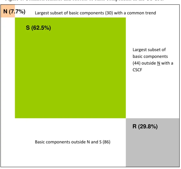
In this paper, we limit our attention to restrictions arising from the fact that non-overlapping subsets of basic components share a common trend (subset N) or a CSCF (subset S). Used in conjunction with bivariate methods, this procedure generates a disaggregation map in which the basic components are classified into subsets N, S and R (see Figure 1). Our work represents a first attempt to build disaggregation maps for the basic components of an aggregate. The results could be useful for several purposes other than forecasting, such as the application of dynamic factors, the formulation of models with unobserved components and the design of economic policies. Indeed, in this paper we apply stationary dynamic factors to the elements in S and the applications will show that we thus obtain better forecasting accuracy for the aggregate than by just applying stationary dynamic factors to the whole set of basic components, ignoring the results of the disaggregation map as is standard practice. The disaggregation map can be extended by including overlapping subsets of basic components with common features and by incorporating, for example, additional common-trend restrictions, the types of common cyclical features identified by Cubadda (2007), common seasonality, co-breaks, common non-linearity, common volatility, etc. We expect to deal with some of those extensions in a future paper.

(9)

Figure 1. Common features and subsets of basic components in the US CPI.a

N (7.7%)

S (62.5%)

R (29.8%)

a The percentages in parentheses refer to the weight in the US CPI of all the basic components in the corresponding subset.

The second and our most important contribution is to develop, along the lines of Giacomini & Granger (2004), a simple indirect forecasting procedure based on single-equation models that departs from the use of vector models, that imposes important restrictions on those models, and that can in practice produce improved forecasts, as we will see in section 5. At the same time, our procedure improves on direct forecasting by including additional relevant information, so that it more than compensates for the greater cost arising from estimation errors in more complex models. We expect this procedure to be widely applicable because it works with the basic components that share selected common features. Moreover, having tested for these restrictions, the basic components that do not share the common features specified in the procedure—subset R—are aggregated5, using the official weights, into an intermediate aggregate rt, which

is forecast by using a scalar model.

We also show that the procedure works when forecasting inflation in three big economies, the US, the EA and the UK. In this context, our work is intended to provide not only better forecasts of an aggregate, but also forecasts of the basic components and of any intermediate aggregates which one could require. These forecasts are useful

5

The aggregation methodology is explained in section 3.2

Largest subset of basic components (30) with a common trend

Largest subset of basic components (44) outside N with a CSCF

(10)

because can be very relevant for policy. The basic elements in R are forecast by using ARI(p,1) models under the restriction that the aggregation of those forecasts gives the direct forecast of the intermediate aggregate rt. This could be done following Guerrero

and Peña (2000).

3. The data

3.1 Data sets and aggregation procedure.

We apply our procedure to the US CPI and the harmonized EA and UK CPIs. These economies were selected because they represent almost 50% of the world GDP and because most econometric applications relate to at least one of these economies. For the US, we use monthly CPI data for all urban consumers, CPI-U, seasonally unadjusted, published by the Bureau of Labor Statistics. The sample goes from January 1999 to December 2010. The aggregate is broken down into 160 basic components. For the EA and UK, we use monthly HICP data, seasonally unadjusted, published by Eurostat. The samples used for the EA and the UK start in January 1995 and finish in December 2010 and the breakdowns of the aggregates have 79 and 70 elements, respectively6. One of the study’s outputs is a disaggregation map based on estimated common features of the basic components. Some intermediate aggregates are formulated from the basic components in the paper, using the official weights and normalizing the sum of the weights of all the basic components in an intermediate aggregate to 100 and applying the normalizing factor to the weight of each basic component in this intermediate aggregate.

3.2. Trend and seasonal factors.

The basic components have trends and some of them seasonal oscillations; therefore we need to test for the presence of positive and seasonal unit roots in the data. To implement these tests to a large number of series we have developed a standard procedure which could automatically be applied to each series. This almost prevents the possibility of considering the presence of outliers when performing these tests and we have ignored the correction for outliers in them. The tests were performed using the log transformation of the data and their results can be found on the website cited in the introduction. We applied the Osborn et al. (1988) tests, hereafter OCSB, and Hylleberg et al. (1990) test as extended in Beaulieu and Miron (1993), hereafter HEGY. Using the terminology employed in the first paper, I(r,s) -where r and s can take values one or zero- means that the data needs r regular differences and s annual differences in order to be stationary. Following both references, we can test whether a particular series is I(1,1), I(1,0), I(0,1) or I(0,0) and in the second and fourth cases if seasonal dummies are significant. All tests are performed at the 99% confidence level and the critical values are taken from Rodrigues and Osborn (1997). Following OCSB test, hypothesis I(1,1) is rejected in all cases except for 4, 9 and 3 basic elements in the EA, US and UK,

6

In all cases the data correspond to the existing published versions in 15th March 2011.

(11)

respectively. Hypothesis I(0,1) is also rejected in most cases, with just 1, 8 and 2 exceptions in the above economic areas. Finally, null hypothesis I(1,0) is only rejected in two cases, one in the UK and another in the US. In the latter hypothesis, the set of seasonal dummies can be appropriate and this can be tested by an F test. In many cases – 24 in the EA, y 17 in US and 14 in UK- the presence of seasonal dummies is not rejected. Thus, based on these results, for the purpose of this paper we consider that all the basic components are integrated of order one and some of them exhibit deterministic seasonality. To corroborate this conclusion we apply the HEGY test. This test refers to the twelve π_i_{coefficients in the notation of Beaulieu and Miron (1993) and the critical}

values were also taken from Rodrigues and Osborne (1997). At the above mentioned confidence level, we get similar results than the ones obtained with OCSB: the need for seasonal differencing is strongly rejected (by an F1,12 test on the null: πi, i=1,..,12, are

zero), but regular differencing is required in all the cases (by a t-test on the null that π₁

is zero). In particular, the null I(0,1) is rejected for all series except one in the EA. The null for a positive unit root is not rejected in any case and the null for eleven seasonal unit roots( by an F2,12 test on the null that πi, i=2,..,12, are zero) is rejected in all cases

but five, four in the basic components of US and one in the EA data, respectively. Since I(1,0) has not been rejected, in these last cases there is a contradiction with the results with the F1,12, but this is something that can occur in finite samples. In sum, the

I(1,0) hypothesis with possible deterministic seasonality seems quite acceptable for the data.

Additionally, applying the ADF test to the differences of the basic components, the null of I(2) for the basic components is rejected in all cases at the 99% confidence level. The critical values are taken from McKinnon (1991) for the case in which a constant is included. This result is as expected, because otherwise innovations in the distant past would have a greater impact on the contemporaneous value of a price index than recent innovations.

In the EA, seasonality in the harmonized index of consumer prices (HICP) has a break at the beginning of 2001 because of a change in Eurostat’s data collection methodology. Thus, in all the tests and models for the EA, following Espasa & Albacete (2007), we always include two sets of seasonal dummies, one of which applies up to December 2000 with the other operating from January 2001. Given the initial 1995– 2003 sample, seasonal change is estimated with few degrees of freedom, so this could be seen as a necessary correction for outliers. With the use of recursive samples – samples in which the initial observations remain fixed but which are enlarged at the end each time that the base of the forecast moves forward- in the forecasting process, seasonal change is ultimately estimated more precisely.

All the models estimated in the following section, even when denoted as ARI, include the appropriate sets of seasonal dummies when required.

4. Our procedure

In our procedure, we distinguish between the following three phases: (1) selection of the relevant common features, which in our case are a stable single common trend and a stable single CSCF; (2) the construction of a disaggregation map, with the largest non-overlapping subsets of basic components sharing one of the above common features; and (3) the construction of single-equation forecasting models for the elements of the disaggregation map.

(12)

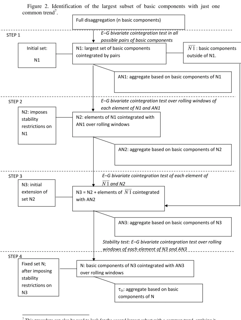
Figure 2. Identification of the largest subset of basic components with just one common trend7.

7

This procedure can also be used to look for the second largest subset with a common trend, applying it to the basic components outside N.

E–G bivariate cointegration test over rolling windows of each element of N1 and AN1

AN1: aggregate based on basic components of N1 Full disaggregation (n basic components)

N1: largest set of basic components cointegrated by pairs

N2: elements of N1 cointegrated with AN1 over rolling windows

E–G bivariate cointegration test in all possible pairs of basic components

AN2: aggregate based on basic components of N2

1

N : basic components outside of N1.

N3 = N2 + elements of N1cointegrated with AN2

AN3: aggregate based on basic components of N3 E–G bivariate cointegration test of each element of

1

N and N2

Stability test: E–G bivariate cointegration test over rolling windows of each element of N3 and AN3

N: basic components of N3 cointegrated with AN3 over rolling windows

τ1t: aggregate based on basic components of N Initial set: N1 N2: imposes stability restrictions on N1 N3: initial extension of set N2 Fixed set N; after imposing stability restrictions on N3 STEP 1 STEP 2 STEP 3 STEP 4

(13)

4.1 Construction of the disaggregation maps

Figure 2 summarizes the process followed to identify the elements in N, the largest subset of basic components with just one common trend. This is done by using cointegration tests based on the Engle–Granger (EG) procedure, although the Johansen test could also be used. Since we have rejected the I(2) hypothesis for the data, the EG tests are performed including a constant and seasonal dummies in the models and the critical values are obtained by simulation following MacKinnon (1991) for sample size of 60 and 108 depending on the economic region at the 90% confidence level8. In the initial step, we apply the cointegration test to all possible pairs of basic components and select the largest subset, say N1, of n0 basic components in which all pairs are

cointegrated. The tests are performed using a restrictive approach for ending up with the presence of bivariate cointegration. Thus, we conclude that two basic components are cointegrated when the hypothesis is not rejected after applying the EG test in both directions.

The second step involves testing whether the bivariate cointegration relationships found in the previous step are stable over time, in the sense that they are evident in shorter subsamples. For this purpose, an intermediate aggregate, AN1, with all the elements of N1 is constructed. Each element of N1 must be cointegrated with AN1 and the stability of this restriction is investigated by estimating and testing for cointegration across the sample by using a rolling window. The elements of N1 that do not pass this “stability test” are removed from N1, and the resulting subset is denoted by N2.

A third step is used to check whether it is possible to enlarge N2. Thus, we consider the basic elements outside of N1 as potential candidates and perform a bivariate cointegration test between each of them and the intermediate aggregate AN2. Any elements that are cointegrated with this AN2 are added to N2 to form a new subset at the end of step 3, termed N3, and the corresponding intermediate aggregate AN3 is constructed.

The final step tests for stability in the bivariate cointegration relationships of the elements of N3, proceeding as in the second step but relating each element of N3 to AN3. Removing from N3 the basic components of N3 that do not pass the test results in the final subset N, which is taken as the largest subset of basic components with only a single (stable) common trend. With the elements of N, the intermediate aggregate τ1t is

formed as it is decribed in section 3.2, and τ1t can be seen as a proxy for the common

trend in the basic components of N.

To apply the procedure proposed by Engle & Kozicki (1993), we look for the largest subset of basic components outside N with just a single CSCF, subset S. The elements of S can be identified by using a four-step procedure similar to that used to identify a common trend, but now testing for a CSCF. With the elements of S, the intermediate aggregate τ2t is formed. In this case, the CSCF can be approximated by the univariate fit

of ∆τ2t, as we did for the purpose of the disaggregation map in this paper, or by applying

the dynamic factor analysis to the components of S.

The disaggregation map obtained from the above results can be represented as a squared n × n matrix, M, the elements of which are arranged in such a way that the

8

The simulated critical values are -3.15 for US, -3.13 for UK and EA, with a unique set of dummies, and -3.33 for EA with two sets of dummies. All critical values are at the 0.1 significance level.

(14)

upper left corner of the matrix collects the n1 basic components with a common trend,

followed by the n2 basic components with a CSCF. In Figure 1, we report the results for

the US. A more detail results for the aggregation maps of US, EA and UK are given in the mentioned website.

The procedure could be extended to identify other subsets of basic components with other types of common trends or CSCFs. For example, one could consider the subset of basic components outside N in which all its elements share two common trends with the elements of N. In addition, the disaggregation map could consider the type of cyclical features identified by Cubadda (2007) as well as other common features such as seasonality, cobreaks, common non-linearities and volatility.

4.2. The final disaggregation maps

The US data used correspond to a breakdown of the US CPI into 160 basic components (listed on the website referred to above). A useful sectorial breakdown of the CPI includes the following sectors: energy (ENE); nonprocessed food (NPF); processed food (PF); non-energy industrial goods (MAN); and services (SERV). We use these “broad CPI categories” to present the disaggregation maps for the basic CPI components. Note, however, that the correspondence is not perfect because a basic component could include prices belonging to two broad categories.

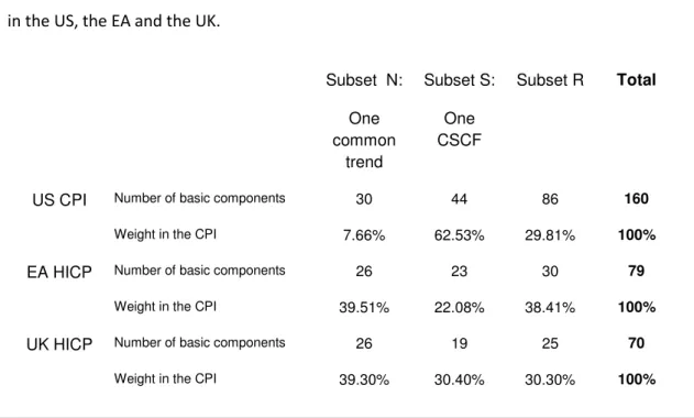
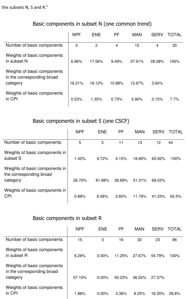
According to Table 1, for the US, the subset N contains 30 basic components that account for 7.66% of the CPI, and belong mainly to MAN (2.90 percentage points (pp)) and SERV (2.15 pp); see Table 2. The number of basic components in subset S—basic components with a CSCF—is 44 and they account for 62.5% of the CPI. The elements of S are more widely distributed among the broad CPI categories; see Table 2. This subset of the disaggregation map has the most weight in the CPI and includes the prices of food, fuels, heat energy, transport and tourism services, nondurable household goods, sporting equipment, and goods related to new technologies. The subset R has 86 elements and they contribute 29.81% to the CPI.

(15)

Table 1. Composition of subsets of basic components sharing one common trend or a CSCF in the US, the EA and the UK.

Subset N: One common trend Subset S: One CSCF Subset R Total

Number of basic components 30 44 86 160

US CPI

Weight in the CPI 7.66% 62.53% 29.81% 100%

Number of basic components 26 23 30 79

EA HICP

Weight in the CPI 39.51% 22.08% 38.41% 100%

Number of basic components 26 19 25 70

UK HICP

(16)

Table 2. Classification by broad categories in the US CPI of the basic components belonging to the subsets N, S and R.a

Basic components in subset N (one common trend)

NPF ENE PF MAN SERV TOTAL

Number of basic components 5 2 4 15 4 30

Weights of basic components

in subset N 6.96% 17.56% 9.49% 37.91% 28.08% 100%

Weights of basic components in the corresponding broad

category 16.21% 18.12% 10.88% 12.67% 3.60%

in CPI 0.53% 1.35% 0.73% 2.90% 2.15% 7.7%

Basic components in subset S (one CSCF)

Weights of basic components in

subset S 1.40% 9.72% 4.15% 18.80% 65.92% 100%

category 26.70% 81.88% 38.89% 51.31% 69.03%

Weights of basic components in

CPI 0.88% 6.08% 2.60% 11.76% 41.23% 62.5%

Basic components in subset R

in subset R 6.29% 0.00% 11.25% 27.67% 54.79% 100%

category 57.10% 0.00% 50.23% 36.02% 27.37%

in CPI 1.88% 0.00% 3.36% 8.25% 16.35% 29.8%

a

(17)

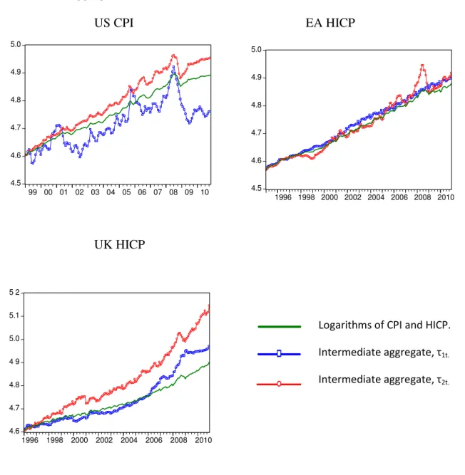
Table 1 also presents results for the EA and the UK. Although they differ from the US results, an important source of this difference is that the US CPI includes (in S) the “owner’s equivalent rent of primary residence” (with a weight in the CPI of around 24%), which the HICPs in the EA and the UK do not include. Nevertheless, correcting for this divergence in CPI composition methods, the basic components with a common trend carry less weight in the US than in the EA and the UK, whereas the basic components with a CSCF carry relatively more weight. In any case, a result that emerges from these applications is that the characteristics of the intermediate aggregates

τ1t, τ2t and rt differ greatly between countries. This is illustrated in Figure 3. In our

sample period, τ1t and τ2t have been diverging considerably in the US and the UK but

not so much in the EA.

Figure 3. Logarithms of CPI (LGCPI) and HICP (LGHICP) and logarithms of the intermediate aggregates τ_1t_andτ_2t_{, for the US, the EA and the UK.}a

US CPI EA HICP

UK HICP

Logarithms of CPI and HICP. Intermediate aggregate, τ1t. Intermediate aggregate, τ2t. 4.5 4.6 4.7 4.8 4.9 5.0 1996 1998 2000 2002 2004 2006 2008 2010 4.6 4.7 4.8 4 9 5.0 5.1 5 2 1996 1998 2000 2002 2004 2006 2008 2010 4.5 4.6 4.7 4.8 4.9 5.0 99 00 01 02 03 04 05 06 07 08 09 10

(18)

5. Forecasting results for inflation in the US, the EA and

the UK

In this section, we apply our procedure to forecast inflation in the US, the EA and the UK9.

5.1. Forecasting procedures

We examine the forecasting results for the year-on-year inflation rates, approximated by the annual differences of the logarithmic transformation of the price indexes. The data are monthly and the samples range from 1995:01 or 1999:01 to 2010:12. The data till December 2003 are used for specification and initial estimation of the models and the remaining data are employed to evaluate the forecasts of the different methods. To do so, we replicate real-time forecasting by using recursive windows for the different forecasting procedures and employing at each step all the available disaggregated information and forecasting up to 12 periods ahead. This means that, by starting with information up to December 2003, we forecast up to December 2004. Then, by extending the sample to January 2004, we test again for the number of lags, check for outliers, re-estimate the models and forecast from February 2004 up to January 2005, and so on. In the forecasting procedures we include dummies for additive outliers.

The forecasting accuracy of each formulation is evaluated by using the root mean squared forecast errors (RMSFEs) at any given forecast horizon. The Diebold & Mariano (1995) test is implemented to test for significant differences between pairs of RMSFEs. In addition, we use the version of the Diebold–Mariano test proposed by Capistrán (2006) based on a multivariate loss function to test jointly the forecast accuracy between two procedures over the 12 horizons.

The following forecasting exercise compares the performance of alternative formulations of the indirect procedures proposed in the paper, and an indirect procedure that uses stationary dynamic factors, against the performance of the direct procedure using an ARI(p,1) for the aggregate variable, called Yt.The direct procedure models the

aggregate variable as a constant, the corresponding deterministic dummies and the own past. All the models include dummies for additive outliers (AO). This is our benchmark model. Stock & Watson (2004, 2007) argue that it is difficult to improve on the results from a simple univariate model with gradually evolving relevant parameters.

∑

= + = ∆ 11 1 log j j j t D

Y α γ (I) constant and seasonal dummies (and

also could include dummies for outliers);

∑

= − ∆ + s j j t j Y 1 log ω

(II) own lags

t

ε

+

(III) residual term

(1)

9

Additional results for all three regions referred to the procedure FP3 estimating the CSCF by the fit of ∆τ_2t_{can be obtained from the above mentioned website.}

(19)

Figure 4. Summary of forecasting approaches.

The models refer to the first differences of the log transformation of the variables.

I) Direct approach

FP1) Forecast the aggregate data by an AR(p) model.

II) Indirect approaches based on the disaggregation map proposed in this paper

FP2) Procedure using a common-trend restriction.

Forecast each basic component of N and the intermediate aggregate formed with the remaining basic components.

FP3) Procedure using a CSCF restriction.

Forecast each basic component of S and the intermediate aggregate formed with the remaining basic components.

FP4) Procedure using a common-trend and a CSCF restrictions.

Forecast each basic component of N and S and the intermediate aggregate formed with the remaining basic components.

III) Indirect approach based on factor-augmented models for the full disaggregation

FP5) Procedure using a stationary dynamic factor.

Forecast each basic component by including a stationary dynamic factor.

IV) Indirect approaches based on AR(p) models

FP6) Forecast each basic component by an AR(p) model like (1).

The forecasting approaches applied in this paper could be classified into four groups, see Figure 4. The first, approach FP1, is the direct procedure, which uses the simplest information set and, therefore, a univariate model for the first differences of the aggregate price index. The model used is given above in equation (1). The second group, comprising approaches FP2 to FP4, includes indirect procedures based on the disaggregation map proposed in this paper. These procedures use different subsets of restricted basic components—N in approach FP2, S in approach FP3 and N and S in approach FP4—and in each case, a specific residual intermediate aggregate is formed from the remaining basic components. Consequently, the residual intermediate aggregates are different under procedures FP2, FP3 and FP4; specifically, it is only under approach FP4 that the residual subset is the subset R, as illustrated in Figure 1. Then, all the basic components selected in each approach are forecast by using the appropriate specification of the general model presented below in equation (3), and the corresponding residual intermediate aggregate is forecast by using an ARI(p,1) model like (1). In the final step, these forecasts are aggregated.

Approach FP3 can be run in two different options corresponding to two approaches for estimating CSCF. One is the fit of ∆_τ_2t_{and the other is by applying the dynamic}

factor analysis to the components of S. Thus the results with FP3 could be compared with those from an application of dynamic factors to all basic components, i.e., ignoring the results from the disaggregation map, as it is done in FP5 below.

The third group, approach FP5, collects indirect procedures based on factor-augmented models, as proposed by Bernanke et al. (2005) and Stock & Watson (2005), for each basic component. Each model is an ARI(p,1) model with stationary dynamic

(20)

factors as regressors. The dynamic factor is estimated over all basic components by applying the procedure described by Stock & Watson (1998, 2002). We obtained the best forecasting results with just one dynamic factor, as did Duarte & Rua (2007). We denote the dynamic factor by Ft. We also found that when using the dynamic factors, a

better forecast of the aggregate is obtained by aggregating the forecasts of the basic components than by forecasting it directly. The general forecasting model used in FP5 for each basic component, xi,t, is as follows:

∑

= + = ∆ 11 1 , , log j j j i i t i D x α γ

(I) constant and seasonal dummies (and also could include dummies for outliers);

∑

= − + k j j t jF 1 λ

(IIa) lags of the stationary factor F_t

∑

= − ∆ + s j j t i j i x 1 , , log ω

(III) own lags

(2)

t i, ε

+

(IV) residual term

The last group, approach FP6, is an indirect procedure based on a univariate ARI(p,1) model for each basic component, similar to the model (1) for the direct procedure.

We are interested in comparing the procedure FP3 proposed in this paper with an indirect procedure that also uses a common factor but that is extracted automatically from the whole set of basic components without having to test for restrictions between these basic components; this is approach FP5. This is the approach that would be followed by those working with dynamic factors from the set of basic components. It is thus interesting to compare it with FP3 where we also use a dynamic factor, but estimated only from the elements in S.

This is important because, as mentioned in the introduction, our procedure incorporates an estimation restriction when calculating the common factors and incorporates a forecasting restriction when forecasting the basic components. In addition, because our procedure allows isolation of the basic components that do not share the common features identified by the analysis, it can directly forecast the intermediate aggregate formed from those (residual) basic components.

The indirect forecasting approaches, FP2 to FP5, require some additional steps in the forecasting process. This is because forecasting the dependent variables requires forecasts of the explanatory variables: common trends, the CSCF and the dynamic factor. For this forecasting exercise, at each forecast horizon, h (> 1) of a given base period n, we need forecasts of those explanatory variables for some periods n + h – j, (h – 1) > j > 0. These are calculated by weighting the forecasts of the corresponding basic components obtained for previous horizons. For the common trend and the CSCF, we use official weights as explained above. We use the loading vector for the dynamic factor. Approach FP3 was used in the two different options mentioned above. The option that estimates CSCF by applying dynamic factors to the elements of S gives better results and is the only FP3 option for which we publish the results here. The comparison of procedures FP3 and FP5 shows the usefulness of applying dynamic factors in the context of a disaggregation map such as that proposed in this paper.

(21)

5.2 Single-equation forecasting models

From the disaggregation map, we need to build single-equation forecasting models for the basic components in N and S and for the intermediate aggregate rt. Then, by

aggregating these forecasts using the normalized official weights of the corresponding CPI as explained in section 3.1, we obtain the headline inflation rate forecast.

The general structure of the forecasting model of the xi,t basic component in N or S is

as follow:

∑

= + = ∆ 11 1 , , log j j j i i t i D

x α γ (I) ∆logxi,t denote the first differences of

the log of i-th basic component. The model include constans and seasonal dummies (could also include dummies for outliers);

) log (log _i_,_t ₁_,_i ₁_,_t i x β τ δ −

+ (IIa) cointegration relationship of basic _component _i_{of N with the intermediate} aggregate τ₁_,_t (3) ) ( 1

∑

= − + S j j t j i λCSCF

θ (IIb) the estimate of the CSCF in S

∑

= − ∆ + k j j t j i 1 , 1 , logτ δ

(IIIa) lags of ∆logτ1,_t

∑

= − ∆ + q j j t j i r 1 , log

ϕ _{(IIIb) lags of}_∆_log

t r

∑

= − ∆ + s j j t i j i x 1 , , log

ω _{(IIIc) own lags}

t i,

ε

+ _{(IV) residual term}

The number of lags is selected based on the Akaike information criterion (AIC). Because we have not tested whether the basic components in N have the same CSCF as that found for the basic components in S, we can now include in the models for the basic components in N the estimated CSCF for S, if this is significant. This is an indirect way of identifying the basic components that share not only the common trend of N but also the CSCF of S. Thus, the models for the basic components in N could include all the terms of the above general structure.

However, because we rejected the hypothesis that the basic components in S have the common trend that is present in N, the models for these components can include all the terms of the general structure (3) except for (IIa).

For the basic elements of R, we proceed, as mentioned above, by forecasting the intermediate aggregate rt directly using model like (1). We do so because in all the

applications described in Section 5.3, forecasting rt directly generates greater accuracy

(22)

5.3. Forecasting exercise

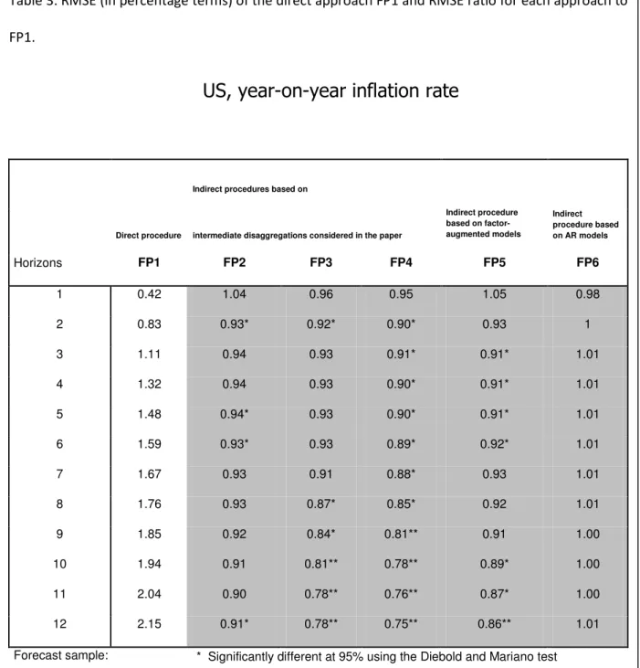
The forecasting results are summarized in Table 3, which in column FP1 reports the root mean squared error (RMSE) of the direct procedure, which is our benchmark. The other columns report the ratios between the RMSEs of the corresponding specific forecasting approaches and the RMSE of FP1. Values below unity indicate an improvement in forecast accuracy with respect to the benchmark model. In this table, a single asterisk (*) indicates that the difference in RMSFEs is significant at the 5% level based on the Diebold–Mariano test and (**) indicates that the difference is significant at the 1% level. In Table 4, we report the Diebold–Mariano test results based on the multivariate loss function proposed by Capistran (2006) to test jointly the forecast accuracy between two procedures over 12 horizons. Tables 5, 6, 7, and 8 reports similar results for EA and the UK.

(23)

Table 3. RMSE (in percentage terms) of the direct approach FP1 and RMSE ratio for each approach to FP1.

US, year-on-year inflation rate

Indirect procedures based on

Direct procedure intermediate disaggregations considered in the paper

Indirect procedure based on factor-augmented models Indirect procedure based on AR models Horizons FP1 FP2 FP3 FP4 FP5 FP6 1 0.42 1.04 0.96 0.95 1.05 0.98 2 0.83 0.93* 0.92* 0.90* 0.93 1 3 1.11 0.94 0.93 0.91* 0.91* 1.01 4 1.32 0.94 0.93 0.90* 0.91* 1.01 5 1.48 0.94* 0.93 0.90* 0.91* 1.01 6 1.59 0.93* 0.93 0.89* 0.92* 1.01 7 1.67 0.93 0.91 0.88* 0.93 1.01 8 1.76 0.93 0.87* 0.85* 0.92 1.01 9 1.85 0.92 0.84* 0.81** 0.91 1.00 10 1.94 0.91 0.81** 0.78** 0.89* 1.00 11 2.04 0.90 0.78** 0.76** 0.87* 1.00 12 2.15 0.91* 0.78** 0.75** 0.86** 1.01

Forecast sample: * Significantly different at 95% using the Diebold and Mariano test 2004/01–2010/12 ** Significantly different at 99% using the Diebold and Mariano test The base periods of the forecasts go from 2003/12 to 2010/11. For horizons 1 and 12, we have 84 and 72 forecasting errors, respectively.

(24)

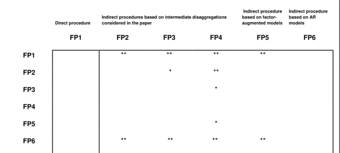
Table 4.Diebold–Mariano test results based on multivariate loss function for the path forecast between two approaches (Capistran 2006): US results.

Direct procedure

Indirect procedures based on intermediate disaggregations considered in the paper

Indirect procedure based on factor-augmented models Indirect procedure based on AR models FP1 FP2 FP3 FP4 FP5 FP6 FP1 ** ** ** ** FP2 * ** FP3 * FP4 FP5 * FP6 ** ** ** **

* Means that the procedure appearing in the column performs significantly better than the procedure appearing in the row at 95%

(25)

EA, year-on-year inflation rate

Indirect procedures based on

Indirect procedure based

intermediate disaggregations considered in the paper on factor-augmented models Indirect procedure based on AR models Horizons FP1 FP2 FP3 FP4 FP5 FP6 1 0.21 0.94* 0.88** 0.85** 0.90* 0.90 2 0.31 0.96* 0.91* 0.91* 0.94 1.27 3 0.41 0.97* 0.92* 0.91* 0.96 1.34 4 0.49 0.99 0.90** 0.89** 0.95 1.32 5 0.58 0.99 0.89** 0.88** 0.93 1.29 6 0.65 1.01 0.89** 0.89** 0.94 1.29 7 0.73 1.01 0.87** 0.87** 0.92 1.21 8 0.81 1.01 0.86** 0.86** 0.91 1.14 9 0.88 1.01 0.87** 0.87** 0.91* 1.09 10 0.94 1.01 0.90** 0.90** 0.92* 1.07 11 1.00 1.01 0.91** 0.90** 0.93* 1.05 12 1.05 1.02 0.93** 0.92** 0.95 1.04

Forecast sample: * Significantly different at 95% using the Diebold and Mariano test

2004/01–2010/12 ** Significantly different at 99% using the Diebold and Mariano test

The base periods of the forecasts go from 2003/12 to 2010/11. For horizons 1 and 12, we have 84 and 72 forecasting errors, respectively.

(26)

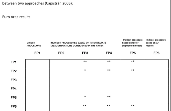
Table 6: Diebold–Mariano test results based on multivariate loss function for the path forecast between two approaches (Capistrán 2006):

Euro Area results

DIRECT PROCEDURE

INDIRECT PROCEDURES BASED ON INTERMEDIATE DISAGGREGATIONS CONSIDERED IN THE PAPER

Indirect procedure based on factor-augmented models Indirect procedure based on AR models FP1 FP2 FP3 FP4 FP5 FP6 FP1 ** ** ** FP2 * ** ** FP3 FP4 FP5 * ** FP6 ** ** **

(27)

UK, year-on-year inflation rate

Indirect procedures based on Indirect procedure based

intermediate disaggregations considered in the paper on factor-augmented models Indirect procedure based on AR models Horizons FP1 FP2 FP3 FP4 FP5 FP6 1 0.27 0.99 0.98 0.98 1.05 0.92 2 0.39 0.97 0.93 0.99 0.98 1.07 3 0.51 0.96 0.91** 0.90* 0.97 1.53 4 0.63 0.94 0.88** 0.84** 0.96 1.38 5 0.75 0.91* 0.86** 0.78** 0.92* 1.24 6 0.86 0.90** 0.85** 0.75** 0.93** 1.19 7 0.97 0.91* 0.84** 0.72** 0.93** 1.16 8 1.08 0.91** 0.82** 0.70** 0.93** 1.14 9 1.19 0.90** 0.80** 0.69** 0.92** 1.12 10 1.3 0.89** 0.79** 0.68** 0.92** 1.11 11 1.39 0.89** 0.79** 0.67** 0.92** 1.11 12 1.49 0.88** 0.79** 0.66** 0.92** 1.11

Forecast sample: * Significantly different at 95% using the Diebold and Mariano test 2004/01–2010/12 ** Significantly different at 99% using the Diebold and Mariano test The base periods of the forecasts go from 2003/12 to 2010/11. For horizons 1 and 12, we have 84 and 72 forecasting errors, respectively.

(28)

6. Conclusions and proposed extensions

6.1 Conclusions

These results, based on CPI data for economic regions that cover about 50% of world GDP, were obtained with a sample of seven years of forecasting errors. Therefore, the results are informative and generate interesting conclusions. The indirect forecast based on using ARI(p,1) models for all the basic components (FP6) is no better than the direct forecast. In fact, for the US, the forecasting performance of FP6 is similar to that of the direct approach for all horizons. In the EA and the UK, FP6 performs relatively poorly for most horizons. Therefore, disaggregation in itself without considering relationships between components does not improve the aggregate forecast in these cases.

In contrast, for the US, the indirect approaches that incorporate information about common features (FP2 to FP4) or about stationary dynamic factors (FP5) perform significantly better than the direct approach for several horizons –all horizons but the first in FP4- (Table 3) and as a whole for the entire forecasting path (Table 4). Similar results are obtained for the EA, except for FP2. For the UK, only approaches FP3 and FP4, which incorporate information about a CSCF and CSCF and the common trend based on the disaggregation map, significantly outperform the direct approach for the entire forecasting path. Moreover, for all three areas and for all horizons, all the indirect approaches, FP2 to FP5 (except FP2 for the EA), have RMSEs below that of the direct method, except in some cases for the one-period-ahead horizon. In addition, in the cases

Table 8: Diebold–Mariano test results based on multivariate loss function for the path forecast between two approaches (Capistrán 2006): United Kingdom results

DIRECT PROCEDURE

INDIRECT PROCEDURES BASED ON INTERMEDIATE DISAGGREGATIONS CONSIDERED IN THE PAPER

Indirect procedure based on factor-augmented models Indirect procedure based on AR models FP1 FP2 FP3 FP4 FP5 FP6 FP1 ** ** FP2 * ** FP3 ** FP4 FP5 * ** FP6 ** ** ** ** **