Comparison between quantile regression technique and generalised additive model for regional flood frequency analysis

(1)

Comparison between Quantile Regression

Technique and Generalised Additive Model for

Regional Flood Frequency Analysis

FARHANA NOOR

STUDENT ID: 18815782

A thesis submitted for the fulfilment of Master of Philosophy Degree

in Western Sydney University, Australia

Principal Supervisor: Associate Professor Dr Ataur Rahman

Co-supervisor: Professor Dr Arumugam Sathasivan

Centre for Infrastructure Engineering

School of Computing, Engineering and Mathematics

Western Sydney University

(2)

A

ABSTRACT

Design flood estimates are needed for the planning and design of hydraulic structures, and in many other water and environmental management tasks. Design flood estimation is a challenging task, in particular for poorly gauged and ungauged catchments. In Australia, there are numerous ungauged catchments; for these catchments Regional Flood Frequency Analysis (RFFA) techniques are generally adopted to estimate design floods.

Most of the RFFA techniques previously adopted in Australia are based on rational method and/or linear modelling approaches. However, with the recent advancements in statistical computation methods, there are several other techniques becoming popular gradually in hydrological applications which can account for non-linearity in the rainfall-runoff processes. Generalized additive model (GAM) is one of the recently developed techniques which can deal with the non-linearity, which has not been widely explored in hydrological research, in particular for the RFFA problems. Therefore, this research is devoted to examining the applicability of GAM in RFFA and compare its performances with one of the most widely used linear RFFA technique (log-log linear model).

This study is carried out using data from 114 small to medium sized gauged catchments of Victoria, Australia. This data has primarily been sourced from Australia Rainfall Runoff (ARR), Project 5 Regional Flood Methods. This study is based on a number of alternative groups, e.g. a combined group consisting of all the 114 catchments and sub-groups formed based on cluster analysis. Four regions are formed using hierarchical and k-means clustering techniques. All the five groups are used for developing log-log linear models and GAM based models. The predictor variables for each of these models are selected based on the statistical significance of the predictor variables, i.e. p-statistics. For validation of the developed prediction models, a 10-fold cross validation method is adopted.

The performances of the prediction models for the alternative models are assessed using a number of statistical measures including coefficient of determination (R2), median relative error (RE) and median Qpred/Qobsratio values. It is found that, none of the models from the

combined group and clustering groups perform equally well for the six average recurrence intervals (ARIs) (2, 5, 10, 2, 50 and 100 years) with respect to the selected statistical measures. Overall, log-log linear model from clustering group A1 is found to be the best

(3)

B performing model. GAM based RFFA models perform better for smaller ARIs (i.e., 2, 5 and 10 years); which is as expected since the hydrological behaviour of catchments for smaller ARIs is generally more non-linear, e.g. higher loss and hence rainfall produces lower runoff for more frequent events.

Some predictor variables (e.g., evap), which were not adopted in the previous RFFA models, in Australia are found to be significant in the GAM based RFFA models. Overall, it is found that consideration of non-linearity via GAM can add new dimensions in RFFA modelling for selecting appropriate predictor variables and to deal with non-linearity.

Overall, the results of this study demonstrate that GAM has a strong potential to enhance the accuracy of RFFA models in Australia; however, additional predictor variables are needed (than what are included in this study) to capture the non-linearity more explicitly between runoff and flood producing variables.

(4)

C

STATEMENT OF AUTHENTICATION

I, Farhana Noor, declare that all the materials presented in this Master of Philosophy Thesis entitled ‘Comparison between Quantile Regression Technique and Generalised Additive Model for Regional Flood Frequency Analysis’ are my own work and that any work adopted from other sources is duly cited and referenced as such.

This thesis contains no material that has been submitted previously, in whole or in part, for any award or degree in other university or institution.

Signed by:

Farhana Noor

(5)

D

ACKNOWLEDGEMENTS

I would like to express my sincere gratitude and thankfulness to my Principal Supervisor, Associate Professor Dr. Ataur Rahman, for the continuous support, guidance and invaluable assistance. He has been a great inspirer for me throughout my MPhil study. This work would not have been possible without his support, encouragement and most importantly the patience during this research. I am also grateful to my Co-supervisor Professor Dr. Arumugam Sathaa Sathasivan and HDR Director, Associate Professor Dr. Dongmo Zhang for their valuable support towards the completion of my research degree. I could not be prouder of my academic roots, and hope that I live up to the research values and the dreams that my supervisors have passed to me.

I would like to thank Australia Rainfall Runoff Project 5 Revision Team to provide me useful data to conduct this study. I would also like to thank to all the staff and fellow researchers at Western Sydney University for their kind support and assistance throughout my research study.

I would not have completed this road if not for my parents, Engr. Mr. Nurul Alam and Advocate Mrs. Zakri Jahan, who instilled within me a quest for knowledge, which has driven me to continue with the research.

Last but not the least, I heart-fully thank and appreciate the constant support and patience of my loving husband Engr. Maruf Adnan during this study. His endless patience and care during the journey will never be forgotten. It would not have been travelled the road to MPhil degree without his constant inspiration.

(6)

E

LIST OF PUBLICATIONS

1. Noor, F., Rahman, A. (2017). Application of Generalized Additive Models in Regional Flood Frequency Analysis: A Case Study for Victoria, Australia, Proceedings of the 1st International Conference on Water and Environmental Engineering, pp. 74-80, 20-22 Nov 2017, Sydney, Australia.

2. Noor, F., Rahman, A. (2018). Comparison of log-log linear model with Generalised Additive model for Regional Flood Frequency Analysis for Victorian Catchments. (In preparation for Natural Hazards)

3. Noor, F., Rahman, A. (2018). Validation of Generalised Additive model for Regional Flood Frequency Analysis in Victoria, Australia (In preparation for 2nd International Conference on Water and Environmental Engineering, 19-23 Jan, 2019, Dhaka, Bangladesh.

(7)

F

LIST OF TABLES

Table 3.1 Descriptive statistics of predictor variables of the selected 114 catchments from

Victoria, Australia ... 34

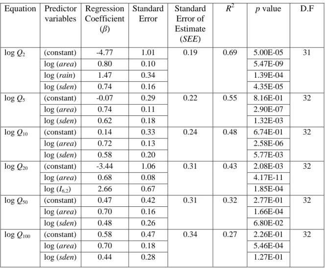
Table 5.1 Model statistics for log-log linear model of combined group ... 66

Table 5.2 Groups Formed by Cluster Analysis ... 70

Table 5.3 Model statistics for log-log linear model of clustering group A1 ... 73

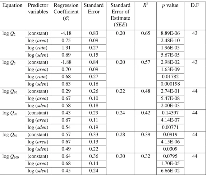
Table 5.4 Model statistics for log-log linear model of clustering group A2 ... 77

Table 5.5 Model statistics for log-log linear model of clustering group B1 ... 82

Table 5.6 Model statistics for log-log linear model of clustering group B2 ... 87

Table 5.7 Median RE values for combined data set and clustering groups ... 92

Table 5.8 Median Qpred/Qobs ratio values for log-log linear model based on combined data set and groupings based on cluster analysis ... 94

Table 5.9 Ranking of log-log linear models ... 96

Table 6.1 Important model statistics for GAM models of combined group ... 101

Table 6.2 Model statistics for GAM model of clustering group A1 ... 106

Table 6.3 Model statistics for the GAM models of clustering group A2 ... 110

Table 6.4 Model statistics for GAM model of clustering group B1 ... 115

Table 6.5 Model statistics for GAM model for clustering group B2 ... 119

Table 6.6 Median RE between combined data and clustering groups for GAM ... 124

Table 6.7 Median Qpred/Qobs ratio comparison between groups for GAM ... 126

Table 6.8 Comparing the overall performance of GAM models ... 126

Table 6.9 R2 values of the GAM and log-log linear models for 10 cases ... 128

Table 6.10 Median RE values (%) for the GAM and log-log linear model based RFFA techniques for ten cases ... 130

Table 6.11 Median Qpred/Qobs ratio values for the GAM and log-log linear model based RFFA techniques for 10 cases ... 133

(12)

K

Table A. 1 Study Catchments of Combined group ... 151

Table A. 2 Study Catchments of Clustering group A1 ... 155

Table A. 3 Study Catchments of Clustering group A2 ... 160

Table A. 4 Study Catchments of Clustering group B1 ... 162

(13)

L

LIST OF FIGURES

Figure 1.1 Flow chart showing major tasks in this research ... 5

Figure 2.1 Various design flood estimation methods ... 9

Figure 3.1 Locations of the selected study area and catchments in Victoria, Australia ... 29

Figure 3.2 Geographical distributions of the selected study catchments ... 31

Figure 3.3 Histogram of catchment area of the selected 114 catchments ... 36

Figure 3.4 Histogram of Streamflow Record Length ... 37

Figure 4.1 Predictive Techniques Explained ... 39

Figure 4.2 RFFA methods (LLLM stands for Log-log linear model, ROI stands for Region of influence and GAM stands for Generalised Additive Model) ... 40

Figure 4.3 Visual Interpretation of GAM ... 43

Figure 4.4 Different Clustering Techniques ... 52

Figure 4.5 Steps in Regionalization using Cluster Analysis ... 57

Figure 5.1 Standardised residual vs fitted predicted value for the log-log linear model for combined group for Q2... 63

Figure 5.2 Normal Q-Q plot for the standardised residuals for the log-log linear model for combined group for Q2... 64

Figure 5.3 Scale-location plot between predicted values and standardised residuals for the log-log linear model for combined group for Q2 ... 64

Figure 5.4 Comparison of observed and predicted flood quantiles for log-log linear model of combined group for Q20 ... 67

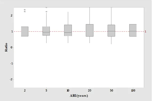
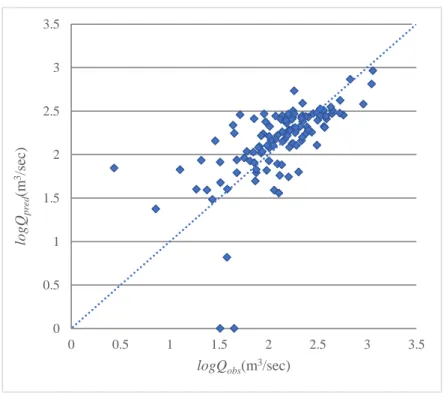
Figure 5.5 Boxplots of relative error RE values for log-log linear model of combined group 68 Figure 5.6 Boxplots of Qpred/Qobs ratio values for log-log linear model of combined group... 69

Figure 5.7 Dendogram Using Ward Linkage Manhattan Distance Between Groups ... 71

Figure 5.8 Comparison of observed and predicted flood quantiles for log-log linear model of clustering group A1 for Q20 ... 74

(14)

M Figure 5.10 Boxplots of Qpred/Qobs ratio values for log-log linear model of clustering group A1 ... 76 Figure 5.11 Comparison of observed and predicted flood quantiles for log-log linear model of clustering group A2 for Q20, ... 79 Figure 5.12 Boxplots of RE for log-log linear model of clustering group A2... 80 Figure 5.13 Boxplots of Qpred/Qobs ratio values for log-log linear model of clustering group A2 ... 81 Figure 5.14 Comparison of observed and predicted flood quantiles for log-log linear model of clustering group B1 for Q20... 84 Figure 5.15 Boxplots of RE values for log-log linear model of clustering group B1... 85 Figure 5.16 Boxplots of Qpred/Qobs ratio values for log-log linear model of clustering group

B1 ... 86 Figure 5.17 Comparison of observed and predicted flood quantiles for log-log linear model of clustering group B2 for Q20... 89 Figure 5.18 Boxplots of RE for log-log linear model of clustering group B2 ... 90 Figure 5.19 Boxplots of Qpred/Qobs ratio log-log linear model values of clustering group B2 . 91 Figure 5.20 Median Relative Error values of log-log linear model based RFFA models based on combined data set and groupings based on cluster analysis ... 93 Figure 5.21 Median Qpred/Qobs values for log-log linear models based on combined data set and groupings based on cluster analysis ... 95 Figure 6.1 Fitted predicted value vs standardised residuals plot for GAM model of combined group ... 98 Figure 6.2 Normal Q-Q plot of the standardised residuals for GAM model for combined group for Q2 ... 99 Figure 6.3 Histogram of the standardised residuals for GAM model for combined group for

Q2 ... 99 Figure 6.4 Comparison of observed and predicted flood quantiles for GAM model of combined group for Q20 ... 102 Figure 6.5 Boxplots of RE values for the GAM model of combined group ... 103 Figure 6.6 Boxplots of Qpred/Qobs ratio values for GAM model of combined group ... 104

(15)

N Figure 6.7 Comparison of observed and predicted flood quantiles for GAM for clustering

group A1 for Q20 ... 107

Figure 6.8 Boxplots of RE values for GAM for clustering group A1 ... 108

Figure 6.9 Boxplots Qpred/Qobs ratio value for GAM for clustering group A1 ... 109

Figure 6.10 Comparison of observed and predicted flood quantiles for GAM for clustering group A2 for Q20 ... 111

Figure 6.11 Boxplots of RE values for the GAM models for clustering group A2 ... 112

Figure 6.12 Boxplots of Qpred/Qobs ratio for GAM model of clustering group A2 ... 113

Figure 6.13 Comparison of observed and predicted flood quantiles for GAM model of clustering group B1 for Q20... 116

Figure 6.14 Boxplots of RE values for GAM for clustering group B1... 117

Figure 6.15 Boxplots of Qpred/Qobs ratio values for the GAM for clustering group B1 ... 118

Figure 6.16 Comparison of observed and predicted flood quantiles for GAM model for clustering group B2 for Q20... 120

Figure 6.17 Boxplots of RE values for GAM for clustering group B2... 121

Figure 6.18 Boxplots of median Qpred/Qobs ratio for GAM for clustering group B2 ... 122

Figure 6.19 Plot of median RE values for different log-log linear and GAM models ... 131

Figure 6.20 Plot of Median Qpred/Qobs Ratio values for the GAM and log-log linear model based RFFA model for multiple datasets ... 134

Figure B.1 Standardised residual vs fitted predicted value for the log-log linear model for combined group for Q5... 168

Figure B.2 Normal Q-Q plot for the standardised residuals for the log-log linear model for combined group for Q5... 169

Figure B.3 Scale-location plot between predicted values and standardised residuals for the log-log linear model for combined group for Q5 ... 169

Figure B.4 Standardised residual vs fitted predicted value for the log-log linear model for combined group for Q10 ... 170

Figure B.5 Normal Q-Q plot for the standardised residuals for for the log-log linear model for combined group for Q10 ... 170

(16)

O Figure B.6 Scale-location plot between predicted values and standardised residuals for the log-log linear model for combined group for Q10 ... 171 Figure B.7 Standardised residual vs fitted predicted value for the log-log linear model for combined group of Q20... 172 Figure B.8 Normal Q-Q plot for the standardised residuals for the log-log linear model for combined group of Q20... 172 Figure B.9 Scale-location plot between predicted values and standardised residuals for the log-log linear model for combined group for Q20 ... 173 Figure B.10 Standardised residual vs fitted predicted value for the log-log linear model for combined group for Q50 ... 173 Figure B.11 Normal Q-Q plot for the standardised residuals for the log-log linear model for combined group for Q50 ... 174 Figure B. 12 Scale-location plot between predicted values and standardised residuals for the log-log linear model for combined group for Q50 ... 174 Figure B.13 Standardised residual vs fitted predicted value for the log-log linear model for combined group for Q100 ... 175 Figure B.14 Normal Q-Q plot for the standardised residuals for the log-log linear model for combined group for Q100 ... 175 Figure B.15 Scale-location plot between predicted values and standardised residuals for the log-log linear model for combined group for Q100... 176 Figure C.1 Comparison of observed and predicted flood quantiles for log-log linear model of combined group for Q2... 178 Figure C.2 Comparison of observed and predicted flood quantiles for log-log linear model of combined group for Q5... 178 Figure C.3 Comparison of observed and predicted flood quantiles for for log-log linear model of combined group for Q10 ... 179 Figure C. 4 Comparison of observed and predicted flood quantiles for for log-log linear model of combined group for Q50 ... 179 Figure C.5 Comparison of observed and predicted flood quantiles for for log-log linear model of combined group for Q100... 180 Figure C.6 Comparison of observed and predicted flood quantiles for log-log linear model of clustering group A1 for Q2 ... 180

(17)

P Figure C.7 Comparison of observed and predicted flood quantiles for log-log linear model of clustering group A1 for Q5 ... 181 Figure C.8 Comparison of observed and predicted flood quantiles for for log-log linear model of clustering group A1 for Q10 ... 181 Figure C. 9 Comparison of observed and predicted flood quantiles for log-log linear model of clustering group A1 for Q50 ... 182 Figure C. 10 Comparison of observed and predicted flood quantiles for log-log linear model of clustering group A1 for Q100 ... 182 Figure C. 11 Comparison of observed and predicted flood quantiles for log-log linear model of clustering group A2 for Q2 ... 183 Figure C. 12 Comparison of observed and predicted flood quantiles for log-log linear model of clustering group A2 for Q5 ... 183 Figure C. 13 Comparison of observed and predicted flood quantiles for log-log linear model of clustering group A2 for Q10 ... 184 Figure C. 14 Comparison of observed and predicted flood quantiles for log-log linear model of clustering group A2 for Q50 ... 184 Figure C. 15 Comparison of observed and predicted flood quantiles for log-log linear model of clustering group A2 for Q100 ... 185 Figure C. 16 Comparison of observed and predicted flood quantiles for log-log linear model of clustering group B1 for Q2... 185 Figure C. 17 Comparison of observed and predicted flood quantiles for for log-log linear model of clustering group B1 for Q5... 186 Figure C. 18 Comparison of observed and predicted flood quantiles for log-log linear model of clustering group B1 for Q10 ... 186 Figure C. 19 Comparison of observed and predicted flood quantiles for log-log linear model of clustering group B1 for Q50 ... 187 Figure C. 20 Comparison of observed and predicted flood quantiles for log-log linear model of clustering group B1 for Q100 ... 187 Figure C. 21 Comparison of observed and predicted flood quantiles for log-log linear model of clustering group B2 for Q2... 188 Figure C. 22 Comparison of observed and predicted flood quantiles for log-log linear model of clustering group B2 for Q5... 188

(18)

Q Figure C. 23 Comparison of observed and predicted flood quantiles for log-log linear model

of clustering group B2 for Q10 ... 189

Figure C. 24 Comparison of observed and predicted flood quantiles for log-log linear model of clustering group B2 for Q50 ... 189

Figure C. 25 Comparison of observed and predicted flood quantiles for log-log linear model of clustering group B2 for Q100 ... 190

Figure D.1 Regression plot by smooth function for predictor variable area for Q2 GAM model... 191

Figure D.2 Regression plot by smooth function for predictor variable I6,2 for Q2 GAM model ... 192

Figure D. 3 Regression plot by smooth function for predictor variable evap for Q2 GAM model... 192

Figure D.4 Regression plot by smooth function for predictor variable sden for Q2 GAM model... 193

Figure D.5 Standardised residual vs fitted predicted values for the Q5 GAM model ... 194

Figure D.6 Normal Q-Q plot of the standardised residuals for the Q5 GAM model ... 194

Figure D.7 Histogram of the standardised residuals for Q5 GAM model ... 195

Figure D.8 Regression plot by smooth function for predictor variable rain for Q5 GAM model ... 195

Figure D.9 Regression plot by smooth function for predictor variable evap for Q5 GAM model... 196

Figure D.10 Regression plot by smooth function for predictor variable sden for Q5 GAM model... 196

Figure D.11 Regression plot by smooth function for predictor variable area for Q5 GAM model... 197

Figure D.12 Regression plot by smooth function for predictor variable I6,2 for Q5 GAM model ... 197

(19)

R Figure D.16 Regression plot by smooth function for predictor variable I6,2 for Q10 GAM

model... 199

Figure D.17 Regression plot by smooth function for predictor variable rain for Q10 GAM model... 200

Figure D.18 Regression plot by smooth function for predictor variable evap for Q10 GAM model... 200

Figure D.19 Regression plot by smooth function for predictor variable sden for Q10 GAM model... 201

Figure D.20 Regression plot by smooth function for predictor variable area for Q10 GAM model... 201

Figure D. 25 Regression plot by smooth function for predictor variable I6,2 for Q20 GAM model... 204

Figure D.26 Regression plot by smooth function for predictor variable area for Q20 GAM model... 204

Figure D.31 Regression plot by smooth function for predictor variable I6,2 for Q50 GAM model... 207

Figure D. 33 Regression plot by smooth function for predictor variable evap for Q50 GAM model... 208

(20)

S Figure D. 34 Regression plot by smooth function for predictor variable area for Q50 GAM

model... 208

Figure D. 39 Regression plot by smooth function for predictor variable rain for Q100 GAM model... 211

Figure D. 40 Regression plot by smooth function for predictor variable area for Q100 GAM model... 211

Figure D.41 Regression plot by smooth function for predictor variable I6,2 for Q100 GAM model... 212

(21)

1

CHAPTER 1 INTRODUCTION

1.1. General

The thesis focuses on the applicability of Generalized Additive Model (GAM) for regional flood estimation. The performance of GAM is compared with the widely used log-log linear model for design flood estimation in ungauged catchments. This chapter begins by presenting a background to this research, need for this research, research questions to be investigated and research tasks undertaken and an outline of this thesis.

1.2. Background of the proposed research

Flood is considered as one of the costliest and disturbing natural disasters. Floods cause loss of lives, economic damage and undermine societal wellbeing (Rahman, 2017). The detrimental impacts from floods can be even worse due to the negative geomorphological impacts of floods, e.g. erosion, sedimentation and destruction of vegetation and wild life. Flooding aftereffects can be substantial on both spatial and temporal scale. In the period 1852 to 2011, 951 people were killed and another 1326 injured by floods in Australia (Carbone and Hanson, 2013). The average annual flood damage is worth over $377 million and infrastructure requiring design flood estimate is over $1 billion per annum in Australia (Gentle et al., 2001). The state of New South Wales (NSW) alone has an average annual cost of flood damage of over $172 million, which is almost 46% of the average annual flood damage cost for Australia. The state of Queensland is second largest in terms of flood damage, with an average annual cost of $125 million. Importantly, the 2010-11 devastating flood in Queensland caused flood damage over $5 billion (Queensland Reconstruction Authority, 2011).

Floods in Australia are triggered by several causes which include excessive precipitation, infrastructure failures and cyclonic effects. Other associating factors that act as drivers to determination of flood magnitudes include catchment and land use characteristics. Rapid

(22)

2 urbanisation, infiltration of waterbodies and land encroachment increase the risk of flooding in a given catchment. Flooding often emerges as a serious threat to livelihoods and infrastructure systems in urban areas due to rapid increase in runoff volume due to larger impervious area and shorter response time. Moreover, climate change has a tremendous impact including more frequent extreme rainfall events resulting in increased flood risk

(Ishak et al., 2013).

Considering the aftermaths of flooding and to ensure the accuracy of a flood forecasting system, the development of a dependable flood risk assessment technique is very important in order to reduce the flood damage cost (Caballero and Rahman, 2014). To develop a reliable flood risk assessment technique, improved methods as well as adequate flood and rainfall data are needed. Flood damage can be reduced if design floods can be estimated more accurately. A well-designed flood infrastructure largely depends on the accuracy of design flood estimation.

Design floods can be defined as the flood discharge associated with a given annual exceedance probability (AEP). Design flood estimation is required in numerous engineering applications, e.g. design of bridge, culvert, weir, spill way, detention basin, flood protection levees, highways, floodplain management, flood insurance studies and flood damage assessment tasks (Aziz et al., 2014). In order to estimate design floods, the most common method used is flood frequency analysis, which requires recorded streamflow data of adequate length at the selected catchment. The accuracy of flood frequency analysis results largely depends on availability of good quality flood data in terms of data quality and quantity. From a statistical point of view, flood estimation from a small sample may give unreasonable or physically unrealistic parameter estimates, especially for probability distributions with a large number of parameters (three or more).

Flood estimation of data poor regions has become a considerable issue in recent years due to effects of some devastating floods in Australia. There are several regional flood estimation methods which have been adopted over the years to estimate the design floods for ungauged catchments. These include Index Flood Method, the Rational Method and Quantile Regression Technique. Regional flood frequency analysis (RFFA) has been considered as one of the efficient methods to ascertain the design flood estimation in data poor regions and

(23)

3 ungauged catchments. This research focuses on regional flood estimation in order to enhance the accuracy of design flood estimates.

Design flood estimation is widely used in practice. At-site flood frequency analysis is used if streamflow data of longer length (generally over 20 years) is available. In many instances, recorded streamflow data is absent or of limited length, and under these circumstances, regional flood estimation methods are adopted. ARR1987 recommended Probabilistic Rational Method in some Australian states. ARR2016 has recommended the RFFE model which is based on regional LP3 distribution where its parameters are estimated using GLS regression. Also, in ARR2016 regions are formed using a region-of-influence approach in the data-rich regions of Australia.

Most of the above RFFA approaches are linear methods, i.e. they cannot incorporate the nonlinearity between floods and flood producing variables. In this regard, GAM can be adopted which can account for the nonlinearity (e.g.,Asquith et al., 2013; Chebana. et al., 2014; Rahman. et al., 2018). In Australia, there has been limited application of GAM in RFFA e.g. Rahman et al. (2018) applied GAM to New South Wales (NSW) state. Hence, this thesis aims to test the applicability of GAM in RFFA to a new region of Australia, which is the state of Victoria. This also compares the performance of GAM based RFFA models with log-log linear models for Victoria.

1.3. Research questions

This thesis is devoted to answering the following research questions in relation to the development of GAM based RFFA models for Victoria.

 Whether the Generalized Additive Model can produce more accurate regional flood estimates as compared to the log-log linear model?

 What is the best set of predictor variables for the development of log-log linear model and GAM based RFFA models?

 Whether cluster analysis can result in better regions for RFFA and reduce uncertainty in RFFA?

(24)

4 1.4. Overview of adopted methodology

To answer the above research questions (identified in Section 1.4), the following tasks are carried out in this study:

 A critical literature review on the most commonly used RFFA and GAM based methods to identify the gaps in the current state of knowledge and further research opportunities in RFFA.

 Selection of catchments from Victoria, collation of streamflow data, selection of catchment characteristics that govern flood generation process and preparation of climatic and catchment characteristics data set.

 Selection of the best performing set of predictor variables for the log-log linear model and GAM based RFFA models.

 Comparison of different candidate regions based on catchment characteristics data using cluster analysis and identification of the best performing region(s) for log-log linear model and GAM based RFFA model.

 Comparison of the performance of the log-log linear model and GAM using a set of independent test catchments.

(25)

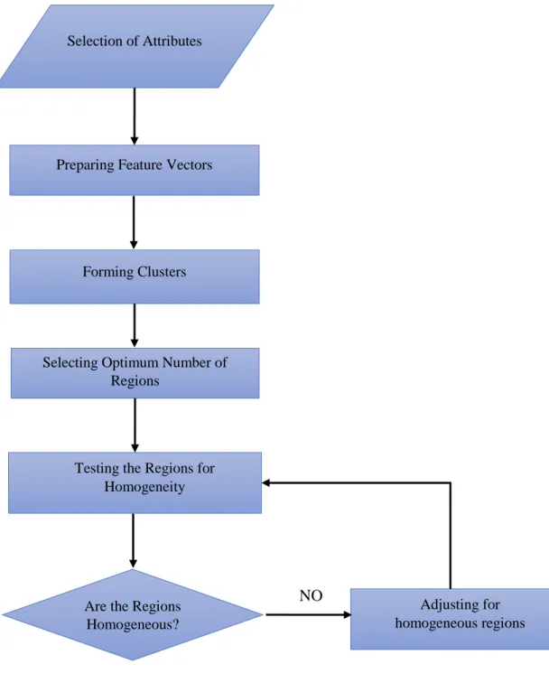
5 Figure 1.1 Flow chart showing major tasks in this research

1.5. Outline of the thesis

The research undertaken in this study is presented in this thesis in eight chapters and four appendices, as outlined below.

Chapter 1 presents a brief introduction to the overall study, includes a background of the proposed research. This chapter also presents the needs for this research, research questions being examined and the main research tasks undertaken to answer the identified research questions.

Literature review

Selection of best performing set of predictor variables

Comparison of different candidate regions based on cluster analysis Selection of catchments and data

collation

Identification of best performing region for log-log linear model and GAM based RFFA model regions

based on cluster analysis

Comparison of the performance of log-log linear model and GAM based RFFA model

(26)

6 Chapter 2 contains a critical review on RFFA techniques with a particular emphasis on GAM, log-log linear model and cluster analysis. At the beginning, various methods of flood estimation are discussed. The review of linear RFFA methods including rational method, index flood method and quantile regression technique are then presented. The GAM is then discussed with a particular emphasis on their applications to hydrology. The assumptions, limitations, advantages and disadvantages of each of the RFFA methods are discussed. The current state of knowledge in RFFA is ascertained and the scopes of further research are identified.

Chapter 3 presents the study area and data collation including data exploration and correlation analysis. The methods of streamflow data preparation are discussed which include gap filling, outlier detection, trend analysis and rating curve error analysis. Selection of catchment characteristics are then presented. The preparation of annual maximum flood series data is described thereafter. Estimation of flood quantiles for average recurrence intervals of 2, 5, 10, 20, 50 and 100 years for the selected gauged catchments by at-site flood frequency analysis is then presented. Finally, a summary of the catchment characteristics data is provided.

Chapter 4 presents the adopted methodologies i.e. GAM, log-log linear model and cluster analysis.

Chapter 5 presents the results of selecting the best set of predictor variables for the development of log-log linear model considering the combined and grouped datasets.

Chapter 6 presents results of selecting the best set of predictor variables for the development of GAM based RFFA models considering combined and grouped datasets.

Chapter 7 presents the comparison of GAM and log-log linear models.

Chapter 8 presents the summary of the research undertaken in this thesis, conclusions and recommendations for further research.

(27)

7

CHAPTER 2 REVIEW OF REGIONAL FLOOD FREQUENCY ANALYSIS

METHODS

2.1. General

Regional flood frequency analysis (RFFA) refers to a generic method of design flood estimation at a target catchment (usually ungauged) by utilizing streamflow records pooled from several other catchments which have similar characteristics with the target catchment. There are many RFFA techniques ranging from simple approximate methods to complex intelligence-based techniques. The purpose of this chapter is to review the concepts of RFFA focusing on estimation of design floods in the range of average recurrence intervals (ARIs) of 2 – 100 years based on linear methods (e.g., quantile regression technique and index flood method) and nonlinear methods (e.g., generalized) additive model. At the beginning, basic issues on design flood estimation are discussed, which is followed by a detailed description of various RFFA methods (index flood method, quantile regression technique and generalised additive models). The model validation techniques are then presented, followed by a description of cluster analysis.

2.2. Basic issues

2.2.1 Design flood estimation methods

Design of water control structures, reservoir management, economic evaluation of flood protection projects, land use planning and management and flood insurance assessment rely on knowledge of the magnitude and frequency of floods, which is referred to as design flood (Srinivas et al., 2007). Often, estimation of design flood is not easy because of paucity of flood records at the sites of interest. The most common methods of design flood estimation include at-site flood frequency analysis (FFA) using observed peak discharge data and event based rainfall runoff modelling.

(28)

8 The design flood can be estimated more accurately for catchments where relatively long streamflow data is available; however, for ungauged catchments (where recorded streamflow data is unavailable or of limited length (less than 10 years) or of poor quality), accurate predictions of design floods remains a challenging task. Moreover, design flood estimates for ungauged catchments are generally associated with a large degree of uncertainty (Haddad and Rahman, 2012).

Error in design flood estimates can lead to undersized or oversized drainage systems, which are equally unacceptable for drainage design; the former results in frequent flooding which cause inconveniences to inhabitants. The latter produces an uneconomical design, which costs more money. Thus, for the design of an efficient and economic drainage system, it is important to estimate design floods accurately.

Selection of particular design flood estimation methods largely depend on the data availability and the purpose of the flood estimation. Lumb and James (1976), Feldman (1979), and James and Robinson (1986) broadly classified design flood estimation methods into two broad categories: streamflow-based methods and rainfall-based methods. These are discussed below and illustrated in Figure 2.1.

(29)

9 Figure 2.1 Various design flood estimation methods

Design Flood Estimation Methods

Rainfall based Methods Streamflow Data Analysis Design Rainfall Historical/ Stochastic Rainfall Deterministic/ Probabilistic Frequency Analysis Design Event Model Runoff Routing Unit Hydrograph SCS Rational Empirical Methods Flood Frequency Analysis Flood Envelop s At Site Regional

(30)

10 2.2.2 At-site flood frequency analysis

At-site flood frequency analysis (FFA), a streamflow-based method, is the most direct method for estimating design floods utilizing the observed peak flow data. The main objective of this method is to develop a relationship between the flood magnitude and annual exceedance probability (AEP) through the use of probability distributions (Chow et al., 1988).

The prime advantage of FFA is that they provide a direct estimate of design floods based on gauged data. Peak flood records represent the integrated response of a catchment to storm events and thus are not subject to the potential for bias that can affect rainfall-based procedures. Furthermore, FFA is quick to apply compared to rainfall-based procedures and have the ability to provide estimates of uncertainty associated with the size of sample and gauging errors. These represent very considerable advantages, and thus it is not surprising that FFA is an important tool for the practicing hydrologists.

However, there are some practical disadvantages with FFA. The available peak flood records may not be representative of the conditions relevant to the problem of interest: changing land-use, urbanisation, upstream regulation, and non-stationary climate are the likely factors that may confound efforts to characterise flood risk. The length of available record may also limit the utility of the flood estimates for the rarer quantiles of interest. Peak flow records are obtained from the conversion of stage data and there may be considerable uncertainty about the reliability of the rating curve when extrapolated to the largest recorded events. In addition, gauges may be relocated, survey datum has been altered, and channel conditions may change, and hence different rating curves are applicable to different periods of historical data. There is also uncertainty associated with the choice of probability distribution which is not reflected in the width of derived confidence limits: the true probability distribution is unknown and it may be that different models may fit the observed data equally well yet diverge markedly when used to estimate quantiles beyond the period of record.

Perhaps the most obvious limitation of FFA is that it relies upon the availability of recorded flood data. This is a particular limitation in urban drainage design as there are so few gauged records of any utility in developed catchments. But the availability of representative records

(31)

11 is also often a limitation in rural catchments, either because of changed upstream conditions or because the site of interest may be remote from the closest gauging station.

FFA methods are most relevant to the estimation of peak flows for very frequent to rare floods. FFA methods can also be applied to other flood characteristics (e.g. flood volume over given duration), but this involves additional assumptions. Peak-over-threshold analysis is most relevant to the estimation of flood exceedances that occur several times a year, up to floods more frequent than around 10% AEP. For rarer events, the use of an annual maximum series is preferred, and with good quality information FFA methods are suited to the estimation of rare floods with AEPs of 2% to 1%. The use of regional flood data provides valuable information that can be used to help parameterise the shape of the flood distribution, and thus where feasible it is desirable to use at-site/regional flood frequency methods. The use of regional information can support the estimation of flood risks beyond 1% AEP and can greatly increase the confidence of estimates obtained using information at a single site. 2.2.3 Regional flood frequency analysis

Regional flood frequency analysis (RFFA) entails estimating design floods at an ungauged site by utilizing flood records pooled from several other catchments, which are similar to the ungauged site of interest. The process of identifying similar catchments for pooling peak flow information is known as regionalization. Research in this area is active over past four decades with new and intriguing findings constantly being reported.

RFFA method can enhance particular site estimates using regional relationships, especially for parameters like skew, which is more prone to sampling error and data extremes. Moreover, regional relationships optimize the effect of outliers which can lead to more reliable extrapolation of flood frequency curve of rarer frequencies. RFFA also enhances the design flood estimates at gauged sites where data may be limited and where direct flood frequency analysis is not feasible.

Various RFFA methods have been adopted in the past such as Rational Method, Probabilistic Rational Method (PRM), Index Flood Method, Quantile Regression Technique, Parameter Regression Technique, and artificial intelligence-based methods (Aziz et al., 2014; Aziz et al., 2015; Bates et al., 1998; Rahman. et al., 2011)

(32)

12 The Rational Method was first introduced by Mulvaney (1851) to estimate peak discharge, which is generally regarded as a deterministic model. However, ARR 1987 recommended a probabilistic form of the Rational Method, known as Probabilistic Rational Method (PRM) for Victoria and Eastern New South Wales (NSW). The PRM in ARR 1987 was based on the

studies by Pilgrim (1982), Pilgrim and McDermott (1982) and Adams (1984). The application of the PRM in ARR 1987 requires a contour map of runoff coefficient. The

runoff coefficient is assumed to vary smoothly over geographic space; however, a sharp variation in the runoff coefficients has been found even within a close proximity indicating discontinuities at catchment boundaries (Pirozzi et al., 2009; Rahman et al., 2008; Rahman and Hollerbach, 2003)

RRFA procedures generally involve the use of regression models to estimate the parameters of probability models (or the flood quantiles) using physical and meteorological characteristics, although simpler scaling functions can sometimes be used for local analyses. Rahman et al. (2015) provided details of a regional flood frequency estimation (RFFE) model for different Australian regions in which the three parameters of the log-Pearson Type 3 model are estimated from catchment characteristics using a Bayesian regression approach. This RFFE model has been incorporated in ARR 2016. The RFFE model provides a quick means to estimate design floods for AEPs ranging between 50% to 1%. The prime advantage of this technique is that it provides estimates of design floods (with uncertainty) using readily available information at ungauged sites; the estimates can also be combined with at-site analyses to help improve the accuracy of the estimated design floods. The prime disadvantage of the technique is that this is only applicable to the range of catchment characteristics used in development of the model, and this largely excludes urbanised catchments and those influenced by upstream impoundments (or other sources of major modification). For such catchments, it will be necessary to consider the use of rainfall-based methods. The RFFE model is quick to apply and provides a formal assessment of uncertainty, and thus is well suited to provide independent estimates for comparison with other design flood estimation approaches.

(33)

13 2.3. Different methods of RFFA

2.3.1. Index flood method

The index flood method is commonly used to develop a flood frequency curve that relates flood magnitude to flood AEP. This method involves scaling a dimensionless flood frequency curve by the index flood. The index flood is a middle-sized flood for which the mean or median of the flood data series is typically used. When the catchment of interest is ungauged, statistical models, such as multiple regressions, are often used to relate the index flood to catchment descriptors.

The index flood method was developed by the US Geological Survey (Dalrymple, 1960) and is based on the technique which relates to the hydrologically similar region. The method extracts data from gauged catchments within a defined region for calculation of parameters for a dimensionless flood frequency curve. The “index flood” of the catchment of interest then scales the curve.

If qT is the dimensionless growth factor, μi is the index flood for site i, then the estimate of the T year flood event at site i, 𝑄_𝑇𝑖 can be estimated by:

𝑄_𝑇𝑖 _{= µ}

𝑖𝑞𝑇 …(2.1)

The index flood, μ, is a middle-sized flood as the mean or median flood (𝑄̅ and Qmed, respectively). The median flood, Qmed, is often preferred as it is a more robust measure than a mean, especially when the index flood must be estimated for a gauged catchment with a short record length. In case of ungauged catchments, the index flood is often estimated through some form of statistical modelling such as multiple regression.

Regression has long been used in hydrology to relate a desired flood quantile to catchment physiographic, geomorphologic and climate characteristics. The analysis is typically performed using the power-form equation:

(34)

14 where QT is the flood quantile of interest, ‘a’ is constant, xi is the ith catchment characteristics,

βi is the ith model parameter, and p is the number of catchment characteristics. In the present context, the quantile of interest is the median flood, which represents the index flood.

A significant amount of research has been conducted in regards to the index flood method both in the past and more recently. Dalrymple (1960) was one of the first researchers to develop an index flood technique which was used by the United States Geological Survey (USGS) prior to 1965. The method developed by Dalrymple (1960) was to relate annual maximum flood series to catchment areas for a particular region of interest. According to the assumption, the flood distribution at different sites was taken constant within a homogeneous region except for a site-specific scale or index flood factor. Homogeneity stands on the concept that the standardised peak floods from different sites in selected regions would follow the common probability distribution with identical parameter values. Relationships were then sought on geographical representation; the particular area was then divided into divisions based on similarity (Riggs, 1973).

The second part of Dalrymple’s approach involved averaging the shapes of similar curves for the region to create one similar common curve; this method was relatively easy to implement as only one variable was required: which was catchment area. As this approach is an empirical one, a number of limitations have been identified:

 Arbitrary decisions are required at boundaries of regions with respect to mean annual flood and the shape of the frequency curve.

 There was no consideration of other important factors which have shown to be plausible/influential in the flood generation process(Riggs, 1973).

According to ARR 1987 (Pilgrim et al., 1987), the index flood method is not encouraged as adesign flood estimation technique for Australia. The assumption has been criticised on the grounds that it is heavily dependent on the idea of regional homogeneity which is not quite satisfactory in the case of Australian regional flood data. The coefficient of variation may vary approximately inversely in terms of catchment area, thus resulting in flatter frequency

(35)

15 curves for larger catchments. The scenario is particularly prominent in the case of humid catchments that differ greatly in size (Riggs, 1973; Smith, 1989).

The index flood method further developed in the late 1980s is a vast improvement to the past methodologies, which use regional average values of LCV and LSK with the at-site mean to fit a GEV or an alternative distribution (Hosking and Wallis, 1997). According to Hosking and Wallis (1997), this approach is effective for the relatively homogeneous region and where record lengths are relatively short. For a finer rating curve, a regional GEV shape parameter can be adopted based upon a regional average. The approach calls a pathway to solve the problems by increasing record lengths and regional homogeneity but at-site data was not long enough to define the shape parameter. Combination of at-site and regional estimators based on each estimator have been proposed as a solution.

Index flood method has been discouraged due to heterogeneity and complexities among Australian catchments. Results show certain discrepancies which is concerning due to concurrent errors in further applications. This provides the ground to further experimentation on other methods where assumptions of homogeneity might be relaxed by considering the spatial variability from site to site within a region.

2.3.2. Quantile regression technique

Regression technique is a simple approach that allows the use of different distributions for different sites in the region. This model develops a transfer function to define a direct relationship between at-site quantiles (outputs) and physio-meteorological variables (predictors or inputs). These techniques have been well suited to ungauged catchment simulations because of their ease of implementation, their rapidity and their good performance. In this regard, numerous models were proposed for RFFA using different transfer functions, including the linear regression model (e.g., Di Prinzio et al., 2011; Holder, 1985; Pandey and Nguyen, 1999; Phien et al., 1990), the generalized linear model (e.g.,Nelder and Baker, 1972), the generalized additive model (Chebana. et al., 2014) and artificial neural networks (Abrahart et al., 2007; Shu and Ouarda, 2007).

The major limitation of regression-based method is that they generally provide only the mean or the central part of at-site flood quantiles. As a result, most of the regression technique

(36)

16 gives the conditional mean of the quantile at ungauged sites considering the physiographic variables (Ouali et al., 2016; Ouarda et al., 2016; Pandey and Nguyen, 1999; Wazneh et al., 2013). Hence, estimated quantiles at gauged sites are commonly used to calibrate the transfer function of the regression model and are not the total representation of full hydrological time series observations.

The USGS adopted an empirical quantile regression method in which a large number of gauged catchments are selected from a region and flow quantiles are estimated from streamflow data, which are then regressed against a set of climatic and catchment characteristic variables that govern the flood generation process. The quantile regression method can be expressed as follows:

𝑄_𝑇 = 𝑎𝐵𝑏_𝐶𝑐_𝐷𝑑 _…_(2.3)

where B, C, D, … are climatic and catchment characteristics variables (predictors) and 𝑄𝑇 is

the flood magnitude with T year ARI, and a, b, c, d, … are regression coefficients.

This method does not require the assumption of a constant coefficient of variation (Cv) of annual maximum flood series in the region unlike an index flood method. It has been noted that the method can give design flood estimates that do not vary smoothly with ARI; however, hydrologic judgement can then be used to make a slight adjustment to the flood frequency curve so that flood estimates increase smoothly with ARI (Rahman, 2005).

Most regional QRTs are based on the methodology published by the USGS. Generally, this method uses a number of gauged catchments in a selected region from which the historical flood records are collected and used in a FFA to provide flood quantiles. Catchment characteristics are then collected for the same gauged catchments. The flood quantiles and catchment characteristics are then used in a regression analysis, which provides an equation that best describes the relationship between the two sets of data. Providing the gauged catchments used in the development of the equations reflect the variability in hydrological behaviour of the catchments in a given region; the equations can then be adopted as a regional flood frequency method.

(37)

17 QRT is particularly applicable for the small to middle-sized catchments where usually data is scarce. For example, if we consider the case of Queensland, it can be observed that there are numerous small catchments which consist of very complex nature of hydrologic and hydraulic characteristics. Therefore, this requires an approach to assess design floods in ungauged catchments using easily-measured parameters for routing drainage design projects. In basic terms, the regression analysis attempts to allocate a proportion of the design flood peak to a particular catchment characteristic. The characteristics used in the regression are required to be hydrologically significant. That is, values must be able to be directly related to either the generation or reduction of rainfall runoff. The parameters should also be easily measured for ungauged catchments to ensure the method is able to be applied as a part of a desktop study.

Catchment characteristics that have been used in QRT studies include catchment area or shape, stream length and slope, vegetation type and quantity, soil type, rainfall depth and intensity, and in some cases, average temperature and catchment elevation. It is also important to note that there are possible inaccuracies in available data, so complex and less significant catchment characteristics may be adding to complexity without adding to the model performance for ungauged catchments. Therefore, only the most dominant characteristics should be adopted.

The USGS flood estimation methods generally use either ordinary least squares (OLS) or more recently the generalised least squares (GLS) method of regression. While the final prediction equations appear similar between the two methods, the GLS is a more complex model than OLS, which is reasonably straightforward in comparison. The GLS method as described by Stedinger (1983) is a regression technique that takes into account the correlation between, as well as differences in, the variability and reliability of the flow estimates used as dependent or response, variables. Whereas the OLS method assumes the model residual is normally distributed, each station is weighted equally, and each site is independent (uncorrelated) (Haddad and Rahman, 2012; Palmen and Weeks, 2011)

Rahman (2005) developed a QRT to test the accuracy of estimating design flood in small to medium sized ungauged catchments in south-east Australia. The study was conducted using

(38)

18 streamflow and catchment characteristics of data of 88 catchments of south-east Australia. The prediction equation for design floods was developed for 2, 5, 10, 20, 50 and 100 years of ARIs based on flood and catchment characteristics data of 88 small to medium sized catchments. A total of 12 explanatory (predictor) variables were adopted for the analyses: rainfall intensity of 12-hour duration and 2-year ARI (I12_2, mm/h), mean annual rainfall (rain, mm); mean annual rain days (rdays), mean annual Class A pan evaporation (evap, mm); catchment area (area, km2); lemniscate shape, a measure of the rotundity of a catchment (shape); slope of the central 75% of the mainstream (slope, m/km); river bed elevation at the gauging station (elev, m); maximum elevation difference in the basin (relief, m); stream density (sden, km/km2), which is the length of stream lines divided by the catchment area; fraction of basin covered by medium to dense forest (forest); and fraction quaternary sediment area (qsa). The developed prediction equations satisfied the underlying model assumptions very well and included hydrologically meaningful predictor variables that are readily obtainable. An independent test indicated that these prediction equations are able to provide reasonably accurate design flood estimates in the study area for small to medium-sized ungauged catchments.

Instead of classical quantile regression approaches, Ouali et al. (2016) proposed a quantile regression model that directly gives the conditional quantile for regional frequency analysis, avoiding using at-site estimated quantiles in the calibration process. The proposed model is able to integrate all the given hydrological information into the calibration step with very short station data record, which is an advantage in the case of poorly gauged catchments. The developed quantile regression model is applied on a dataset representing 151 hydrometric stations from the province of Quebec and compared with a classical regression model. Monte Carlo simulation method has been used to quantify the at-site estimation error and to assess the impact of record length on model accuracy. Application of this test to the annual maximum streamflow series for each gauged station indicates that three stations of 151 are found to be nonstationary at a significance level of 1%. Given the small percentage of rejected stations (2%), and to maximize sources of information; these stations have been retained in this study. In a nutshell, the model has proven to be a feasible model for regional flood estimation.

(39)

19 Different types of regression analysis

There are several methods to estimate regression coefficients including ordinary least squares (OLS), generalised least squares (GLS) and weighted least squares (WLS) methods.

Ordinary least Square (OLS) Method:

OLS method is widely adopted in regression analysis. This is considered as one of the simplest methods for estimation of regression coefficients. It attempts to find the best fitting regression coefficients by minimising the sum of squared residuals. The OLS model can be expressed as:

Y = Xβ + e …(2.4)

where Y is a (n × 1) matrix of flow characteristics at N sites, X is a (n × k) matrix of catchment characteristics augmented by a column of ones, β is a (n x 1) vector of regression parameters and e is an (n x 1) vector of random errors assumed to be normally distributed with zero mean and the covariance matrix assumed to be of the form INσ², where IN is a N–

dimensional identity matrix. The OLS estimate of β is:

βols = (X′X)-1X′𝑌̂ …(2.5)

The sampling covariance matrix based on the above assumptions can be expressed as:

Var( 𝛽̂ols) = σ2(X ′ X )

−1 _…(2.6)

The OLS estimator is generally used by hydrologists to estimate the parameters β in Equation 2.5. The accuracy of estimation by OLS in RFFA by QRT depends on several assumptions: • The annual maximum flow at each of the sites are not correlated;

• The record lengths should be equal for all the sites; and

(40)

20 These assumptions are very unlikely to be satisfied for hydrological regression analysis. In order to overcome the problem that has arisen from the OLS regression, Stedinger and Tasker (1985) proposed the GLS regression procedure which can result in remarkable improvements in the precision with which the parameters of regional hydrologic regression models can be estimated, in particular when the record length varies widely from site to site.

Generalised least squares (GLS) regression

Regression using hydrological data violates the assumption of OLS procedure that the residual errors associated with the individual observations are homoscedastic and independently distributed (Stedinger and Tasker, 1985). Variations in streamflow record length and cross-correlation among concurrent flows, resulting in estimation of T year events which is likely to vary in precision. Moreover, from the former studies it is found that, OLS estimates of the standard error of prediction and the estimated parameters are highly biased. GLS regression method is an effective way to deal with these problems.

Stedinger and Tasker (1985) used Monte Carlo simulation to show the superiority of the GLS procedure to derive empirical relationships between streamflow statistics and physiographic basin characteristics. A further extension of the GLS method was presented by Tasker and Stedinger (1989) which included the realities and complexities of regional hydrological data sets that were not addressed in the Monte Carlo simulation studies. These extensions incorporated (1) a more realistic model of the underlying model error; (2) smoothed estimates of cross correlation of flows; (3) procedures for including historical flow data; (4) diagnostic statistics describing leverage and influence for GLS regression. Therefore, it is preferable to develop GLS regression model employed by Stedinger and Tasker (1985) integrating these new extensions especially in regards to identifying the realistic model error associated with the GLS analysis. The GLS procedure as described by Stedinger and Tasker (1985) and Tasker and Stedinger (1989) require an estimate of the covariance matrix of residual errors 𝛴̂(Y) whose elements are organised in a matrix as follows:

𝛴̂(𝑌) = { σ_𝑖2 𝑛𝑖[1 + 𝐾𝑇 2 (𝜅−1) 4 ] 𝑓𝑜𝑟 (𝑖 = 𝑗) 𝜌𝑖𝑗𝑚𝑖𝑗 _𝑛σ̂𝑖σ̂𝑗 𝑖𝑛𝑗 [1 + 𝜌𝑖𝑗𝐾𝑇 2 (𝜅−1) 4 ] 𝑓𝑜𝑟 (𝑖 ≠ 𝑗) …(2.7)